Abstract
The effects of the emissions of anthropogenic greenhouse gases (GHGs), aerosols, and natural forcing on the summer-mean surface air temperature (TAS) in the East Asia (EA) land surface in the 20th century are analyzed using six-member coupled model inter-comparison project 5 (CMIP5) general circulation model (GCM) ensembles from five single-forcing simulations. The simulation with the observed GHG concentrations and aerosol emissions reproduces well the land-mean EA TAS trend characterized by warming periods in the early (1911–1940; P1) and late (1971–2000; P3) 20th century separated by a cooling period (1941–1970; P2). The warming in P1 is mainly due to the natural variability related to GHG increases and the long-term recovery from volcanic activities in late-19th/early-20th century. The cooling in P2 occurs as the combined cooling by anthropogenic aerosols and increased volcanic eruptions in the 1960s exceeds the warming by the GHG increases and the nonlinear interaction term. In P3, the combined warming by GHGs and the interaction term exceeds the cooling by anthropogenic aerosols to result in the warming. The SW forcing is not driving the TAS increase in P1/P3 as the shortwave (SW) forcing is heavily affected by the increased cloudiness and the longwave (LW) forcing dominates the SW forcing. The LW forcing to TAS cannot be separated from the LW response to TAS, preventing further analyses. The interaction among these forcing affects TAS via largely modifying the atmospheric water cycle, especially in P2 and P3. Key forcing terms on TAS such as the temperature advection related to large-scale circulation changes cannot be analyzed due to the lack of model data.
1. Introduction
Intense research in the recent decades confirmed that the increase in the global-mean surface air temperature (TAS), most notably since early 20th century, has been caused by the emissions of anthropogenic greenhouse gases (GHGs) and aerosols/aerosol precursors from industrial sources with minimal contributions from the natural variability [1,2,3,4,5,6]. The human-induced climate change affects a wide range of sectors, both human and natural, over the globe. Because of wide-spread impacts on the human society and the natural ecosystems, understanding the ongoing climate variations and projecting future climate have become an important practical concern worldwide [7], especially for developing the plans for mitigating and adapting to the impacts of future climate change on human sectors and natural ecosystems.
Geographical variations in the temperature trend are an important concern for regional policymakers as the timing and magnitude of temperature changes are crucial in shaping the climate change impacts on specific sectors of regional interests [8]. Although generally positive, the observed temperature trend over the 20th century varies strongly according to regions [7,9]. The time series of the 20th century land-mean temperature from the observation-based records show smooth increasing trends for the entire globe (black line with open circle in Figure 1a) disrupted by a slight cooling episode between the mid-1940s and the early 1970s. Similar variations in the land-mean TAS during the 20th century also occur over East Asia (EA; black line with open circle in Figure 1b); the magnitude of the overall warming trend and the mid-20th century disruption of the warming over EA are much more pronounced than for the entire globe. The impacts of GHGs and aerosols on TAS vary widely according to the radiative properties of each species and associated feedback within the climate system. Thus, the observed variations in the 20th century temperature for EA in Figure 1b may be related, at least partially, to the history of human activities in the region during the period.
Combustion of fossil fuels has increased the atmospheric carbon dioxide (CO2) concentration from 280 ppm before the Industrial Revolution to 400 ppm in early 21st century, resulting in positive radiative forcing (RF) to the climate system [7,9,10]. Combustion of fossil fuels also emits aerosols and aerosol precursors, most importantly black carbons, sulfur dioxides, and nitrous oxides. Aerosol radiative forcing also affects the energy budget and TAS in a complicated way according to the radiative properties of each aerosol type. For example, absorbing aerosols such as black carbons heat the atmosphere by absorbing the solar radiation, while the reflecting aerosols such as sulfates reduce the overall absorption of the solar radiation by the Earth [11,12]. Previous studies [4,13,14,15,16] estimated that the overall RF on the climate system by anthropogenic aerosols range from −0.22 to −1.85 Wm−2. The effects of the aerosol RF on climate also varies by seasons and regional climate characteristics [17,18]. In addition to the direct aerosol RF, aerosols also affect the Earth’s energy budget indirectly by altering clouds. Thus, the overall RF associated with anthropogenic emissions is a consequence of interplay of GHGs and aerosols of various optical properties as well as their impacts on other elements of the climate system, especially clouds.
Long-term climate variations over EA are an important concern, not only for the region but also for the entire world. The region of dense population has been prone to severe damages from weather-related natural disasters such as flooding and drought. Temperature variations affect food productions in EA, a region of marginal food production for supporting its large population. Rapid economic developments in recent decades made EA a major source of anthropogenic GHGs and aerosols in the world [19,20,21]. The larger temperature variations in the 20th century over EA compared to the rest of the entire globe (Figure 1b) is of particular concern as it may indicate more extreme temperature variations in the future. The large temperature variations in EA during the 20th century may be related to the history of anthropogenic aerosol emissions within the region because, due to their short life span, the RF of aerosols tend to be more regionally confined than that of GHGs [3,22,23]. Considering critical impacts of aerosol RF on the water cycle over EA such as the EA summer monsoon [24,25,26,27,28,29,30,31,32], understanding the RF associated with anthropogenic emissions of GHGs, aerosols, and aerosol precursors is a key step in identifying the causes of historical TAS variations and future changes over EA [33].
This study aims at assessing the relationship between the long-term variations in the summer TAS and the corresponding variations in RF by the emissions of anthropogenic GHGs, aerosols and natural forcing related to volcanic eruptions and solar activities during the 20th century, using the fifth Coupled Model Intercomparison Project (CMIP5) transient simulations. The summer TAS is closely related to a variety of key sectors in EA including agriculture, water supply and demands, and natural ecosystems. Unlike most previous studies which assess the GHG and aerosol effects, as well as their interactions, under equilibrium states [23,34], this study attempts to understand the response of TAS to more realistic variations in the anthropogenic GHG, aerosols, natural forcings, and the internal variability of the climate system, using transient simulations. Song et al. [35] attempted to study the effects of the observed variations in the GHGs and aerosol forcing on the EA climate using CMIP5 simulations for three different simulations with historical, historical GHG, and historical natural forcing; however, their study based on the linearity assumption cannot separate the nonlinear interactions from the aerosol forcing. This study is designed to explore the effects of GHGs, anthropogenic aerosols, and natural forcing explicitly with separate aerosols forcing runs, so that the effects of interactions among these forcing in shaping the observed TAS variations over EA in the 20th century can be account for. We have analyzed a total of 30 simulations from 6 CMIP5 models for five different simulations with historical, historical GHGs, historical anthropogenic aerosols, and historical natural forcings, and a pre-industrial (PI) conditions in order to assess separately the effects of anthropogenic GHGs and aerosols, as well as natural forcings and internal variability on TAS over EA. The CMIP5 models and experiments setup are described in Section 2. It is followed by the analyses of the model data in Section 3. Summaries and Discussions are presented in Section 4.
2. Data and Methodology
2.1. Model Data
In this study, we use 30 simulations from 6 GCMs contributing to phase 5 of the Coupled Model Intercomparison Project (CMIP5) through the Earth System Grid Federation following Taylor et al. [36]. The model names, institutions, and resolutions are listed in Table 1. All the model outputs are bilinearly interpolated into horizontal resolution of 2.81° × 2.81° grid, which is the same as grid of the Canadian Earth System Model 2 (CanESM2) model. The bilinear interpolation tends to underestimate local maxima but does not create fictitious local peaks, either. The multi-model ensemble (MME) is examined by the arithmetic mean of model output, with the same weight for each model. Five experiments of different forcing are selected for each model: the historical simulation (HST) is forced by observed history of the anthropogenic GHGs and aerosols as well as the natural forcing by the solar and volcanic activities. The single-forcing runs using only the historical GHGs (GHG), anthropogenic aerosol emissions (AER), and natural forcing (NAT) are used to estimate the effects of these individual forcings on TAS. The effects of the internal variability of the climate system (INT) is estimated from the Pre-industrial (PI) simulation in which the solar constant is fixed as a constant, no volcanic activities are considered, and the GHG and aerosol concentration are fixed at the PI level. Each GCM provides a single member to each ensemble. More details are described below Section 2.3.

Table 1.
The descriptions of the CMIP5 models used in this study.
2.2. Observational Data
This study employs temperature indices derived from high-resolution (0.5° × 0.5°) monthly-mean temperatures from the Climate Research Unit (CRU) TS version 3.2.2. [43] for the reference for evaluating the simulated land-mean temperatures. The CRU dataset is based on analyses of temperature data at surface stations and covers the global land surface except Antarctica. The CMIP5 simulations used in this study account the temporal variations in the solar and volcanic activities towards the natural forcing. The solar activities are prescribed from the annual mean time series of sunspot number from the Solar Influences Data Analysis (SIDC, Royal Observatory of Belgium) and the annual mean time series of total solar irradiance data from NOAA [44,45,46]. The effects of volcanic eruptions on TAS are accounted in terms of the radiative effects of volcanic ashes by prescribing the monthly mean time series of the stratosphere aerosol optical depth (SAOD) dataset from the National Aeronautics and Space Administration/Goddard Institute for Space Studies (NASA/GISS) [33,47,48].
2.3. Methodology
This study explores the effects of anthropogenic (by the emissions of aerosols and GHGs) and natural (by the solar and volcanic activity) forcings on the historical variations of the summer TAS in EA in the 20th century. For a given climate variable Ψ, the amount of variations over a time period (ΔΨ) that are associated with the changes in anthropogenic aerosol concentration (Δα), the GHGs concentrations (Δg), and the natural forcings (Δn) may be decomposed as in Equation (1) below:
where R(Δα, Δg, Δn) is the change due to the nonlinear interactions between Δα, Δg and Δn, and I is the changes due to internal variability. The first three terms on the right hand side of Equation (1) represent the changes in Ψ solely by the forcing from anthropogenic aerosols, GHGs, and natural events (the solar and volcanic activities) in order.
ΔΨ(Δα, Δg, Δn) = (∂Ψ/∂α) Δa + (∂Ψ/∂g) Δg + (∂Ψ/∂n) Δn + R(Δα, Δg, Δn) + I
The five term in Equation (1) are estimated using the six-model ensembles from five sensitivity simulations for the period 1860–2005 (Table 2). The first simulation from which ΔΨ(Δα, Δg, Δn) is calculated accounts for the historical variations in the emissions and concentrations of aerosols, GHGs, and natural forcing; i.e., the most realistic representations of all forcings (HST) on TAS. Details of the forcing agents (GHGs, Aerosols, and Natural, etc.) in CMIP5 models are described in Table S1 of the supporting information. Three single-forcing simulations (Table 2) are used to calculate the first three terms on the right hand side of Equation (1). The anthropogenic aerosol-only simulation (AER) accounts for the historical anthropogenic aerosol emissions while the GHGs concentrations are fixed at the 1860 level. The GHG-only simulation (GHG) implements the historical GHGs concentration while anthropogenic aerosol emissions are fixed at the 1860 level. The natural forcing run (NAT) implements the historical natural forcing due to the solar activity and volcanic eruptions while the GHGs and aerosol concentrations are fixed at the 1860 level. In addition, the PI simulation (INT), where both the concentration of the anthropogenic aerosols and GHGs as well as the natural forcings are fixed at the pre-industrial (1860) level, is employed to assess the effects of the internal variability of the climate system on the TAS variations.
Table 2.
Five sets of climate simulations are used in this study.
Because internal variabilities of various time scales can play an important role in modulating regional temperature and characterizing the individual model uncertainties, we first examined the significance of internal variabilities of 30-year and 150-year timescales using the Pi-control runs. The trend of the 6-model ensemble temperature over the 150-year period is much smaller than those from the simulations listed in Table 2 and the corresponding residual term (not shown). For estimating the trends at 30-year time scales, we randomly selected 100 samples of consecutive 30-year periods and calculated 30-year trends for individual samples. The 30-year trends calculated for the 100 samples are used to calculate the mean and the standard deviation of the 30-year trend. This step was necessary because the Pi-control runs are not tied to real calendar, i.e., the Pi-control runs cannot be related to specific periods. The mean 30-year trends over the 100 samples are nearly zero; i.e., negligible compared to the effects obtained in the simulations and the corresponding residuals. The uncertainty of the 30-year trends due to the internal variability, estimated by the standard deviation of the 30-year trends of the 100 samples is also smaller than most terms except the effects of aerosols in P1 and the effects of the natural forcing term in P3. The uncertainty range is presented by the two dashed black lines in Figure 1c. Note that the effects of aerosols and the natural forcing in P1 and P3, respectively, are negligible compared to the effects of other forcings in the same period. Based on the analysis above, we concluded that the effects of internal variability on the temperature trend in each period can be neglected.
A detailed description of the CMIP5 simulation design is provided by Taylor et al. [36]. These five simulations allow us to estimate all five terms in Equation (1). The residual term R (the fourth term in the right-hand-side of Equation (1)) that represents the nonlinear interaction of anthropogenic (GHG, aerosol) and natural forcings is calculated by subtracting the sum of the single forcing experiments AER, GHG, NAT and INT from HST. The CMIP5 model data are analyzed for the East Asia region covering 20°–50° N and 110°–140° E which includes eastern China, Korea, Japan, and Manchuria. The summer climate is represented by the average over the three summer months, June, July, and August. Statistical significance level is determined based on the Mann-Kendall trend test. Based on the observed TAS variations in Figure 1b, we select three 30-year periods based on the TAS trend variations: 1911–1940 (P1: warming), 1941–1970 (P2: cooling) and 1971–2000 (P3: warming). We explore the effects of the anthropogenic GHGs and aerosols, natural forcings, as well as their interactions, on the temperature records for each period from the simulated data. The variations of the selected variables in the three periods are represented by the trends over the corresponding periods.
3. Results
3.1. Evaluation of the 20th Century Overland Temperature in HST
The interannual variations of the land-mean TAS in HST are compared against the CRU data for the entire globe (Figure 1a) and for EA (Figure 1b). HST is run with the observed emissions of well-mixed GHGs, anthropogenic aerosols, and natural agent change (solar and volcanic) during the simulation period; thus is expected to generate the most realistic TAS among the five simulations. The observed TAS over the EA land region (Figure 1b) is in-phase with the global TAS (Figure 1a), but with more pronounced variability during the middle (1941–1970) of the 20th century period. For both the global and EA land surfaces, HST well depicts the long-term TAS variations characterized by a positive TAS anomaly peak in the 1940s and a negative peak in early 1970s followed by continuous increases in the late 20th century period. The model performs better for the global mean than for the EA-mean; the correlation coefficient between the observed and the TAS time series in HST is 0.95 for the global land surface and 0.68 for the EA land surface. The five sensitivity simulations show that the simulated TAS variations during the 20th century primarily result from the warming effects of GHG increases and the cooling effects of anthropogenic aerosols (red and blue lines, respectively, in Figure 1a,b). The natural forcing by the solar activity and volcanic eruptions also contributed to the warming trend in early 20th century and the cooling trend in mid-20th century (green lines in Figure 1a,b). Details of the TAS trends in individual sensitivity experiments will be discussed in the following sub-sections.
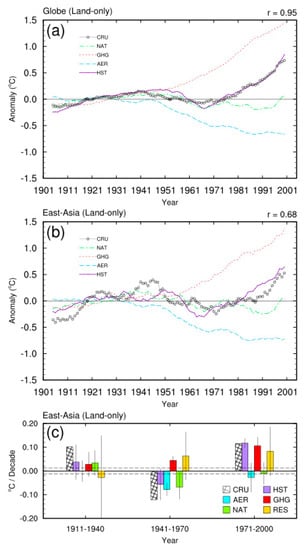
Figure 1.
The June to August (JJA)-mean surface air temperature (TAS) time series in the 20th century from Climate Research Unit (CRU) and the GCM simulations over the land surface of (a) the entire globe and (b) EA, and (c) the linear trend of TAS obtained from the simulations in Table 2 and the corresponding residuals for the three periods. In (a) and (b), the 10 year running-mean TAS anomaly (1901–2005) over the entire globe and EA are shown. CRU indicates the CRU data and RES is the residual term calculated from the simulations as Equation (2); abbreviations for other runs are the same as in Table 2. Error bars indicate the standard deviation of CMIP5-model multi-model ensemble (MMEs) from each simulation. The black dashed horizontal lines indicate the range of the internal variability on the 30 year timescale estimated as one standard deviation of the 30-year trends of the 100 samples from the Pi-Control MME as described in Section 2.
3.2. TAS Trends Related to Anthropogenic Emissions
The TAS trend in the four sensitivity simulations (HST, AER, GHG, and NAT) are compared against the observed trend for the three periods defined in Section 3.1 (Figure 1c). The mean 30-year internal variability estimated from the Pi-control runs is negligible; the range of the TAS trend due to internal variability is presented by the black dashed lines in Figure 1c. The TAS trend in HST is different from the sum of the trends in the single-forcing simulations. These differences arise due to the interactions among the individual forcing elements that cannot be simulated in the single-forcing runs. The residual term R in Equation (1) that arises from interactions among the individual forcing elements, is estimated from the five sensitivity simulations as in Equation (2) below:
RES = HST − GHG − AER − NAT
Note that the internal variability term (INT) is neglected in calculating the RES term in (2) as its contribution to the TAS trend is negligible compared to the contribution from other forcings. The sign of the linear trend of TAS in HST (purple bar in Figure 1c) agrees with that derived from the CRU data (black hatched bar in Figure 1c) for all of the three 30-year periods despite some differences in the magnitude. Results from the historical (HST) and the three single-forcing simulations (GHG, AER, and NAT) and the residual term (RES) obtained from Equation (2) are analyzed to assess the effects of GHGs, anthropogenic aerosols, natural forcings and their nonlinear aspects on the TAS variations during the 20th century in the following sub-sections.
3.2.1. TAS Variations in P1
The first 30-year period 1911–1940 (P1) is characterized by a rapid increase in TAS (Figure 1b), mainly due to the natural forcing (increasing solar irradiance and decreasing volcanic aerosols) and the increase in GHGs as the main contributors to the positive TAS trend (Figure 1c). Anthropogenic aerosols exert almost negligible effects on TAS in P1. The interaction term (RES) is negative in P1 but is smaller in the magnitude and is of much larger statistical uncertainty compared to GHG and NAT. Thus, the positive TAS trend during P1 mainly results from the combined warming effects of the natural forcing and GHG increases exceeding the cooling effects of the interaction term. The global CO2 concentration (red dashed line) and EA SO2 emission (blue solid line) profiles implemented in the HST, AER and GHG runs show that both the CO2 concentration and the increase in the East Asian SO2 emission is in P1, a pre-industrial period for most of EA, is much lower than in P2 and P3 in which heavy industrialization has occurred in EA (Figure 2). This results in smaller effects of GHGs and aerosols on the TAS variations in P1 (early 20th century) than in P2/P3 (middle/late 20th century). The positive contribution of the natural variability to the warming trends in P1 is a part of the long-term recovery of TAS from the large cooling by the massive volcanic activities in late 19th/early 20th century (the Krakatoa 1883, the Santa Maria 1902, the Mt. Katmai 1912 in Figure 3b) [45,47,49]. The solar activity has also increased in P1, but the magnitude is small. Details of the solar activity and volcanic eruptions implemented in the CMIP5 natural forcing are referred to Moss et al. [50].
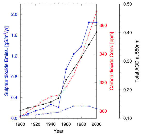
Figure 2.
The time variation of the historical emissions of anthropogenic sulphur dioxide and carbon dioxide from 1900 to 2000 based on the RCP database v2.0.5 [51] and the simulated aerosol optical depth from CMIP5 models. The global sulphur dioxide emission (blue dashed line with open circle), the Asian emissions (blue solid line with closed circle) are shown; the black line indicate the total aerosol optical depth at 550 nm in JJA over East Asia.
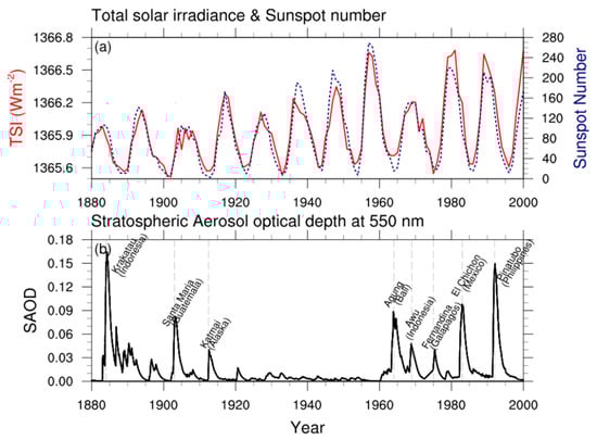
Figure 3.
Time variation of (a) total solar irradiance (TSI; red solid line) for CMIP5 & observed sunspot number (blue dotted line), (b) stratospheric aerosol optical depth at 550 nm (SAOD) from 1880 to 2000. Annual mean TSI time series provided from National Oceanic and Atmospheric Administration (NOAA). Sunspot data from Solar Influences Data Analysis Center (SIDC, Royal Observatory of Belgium). Monthly mean stratospheric aerosol optical depth (SAOD) dataset used from NASA Goddard Institute for Space Studies (GISS). Dotted vertical gray lines denote the times of maximum SAOD during major volcanic eruptions.
Warming trends in P1 are observed in most of the EA land region, particularly in the Manchuria, the Korean Peninsula, far-eastern Russia, and Japan, except the Mongolia region (Figure 4a). The simulated TAS trends in P1 show large regional variations over EA. The simulated TAS in HST also shows positive trends over the land in P1 but the trends are smaller than from the CRU data (Figure 4b). These TAS trend closely coincides with the TAS response to the natural forcing (NAT), especially over northeastern and southern China (Figure 4e). For the East Sea of Korea, much of the warming by GHG increases (Figure 4d) is offset by the cooling by anthropogenic aerosols (Figure 4c). Note that statistically significant TAS trend in both AER and GHG occurred mainly over the seas around Japan (Figure 4c,d). The interactions between the anthropogenic and natural forcings (Figure 4f) result in very weak negative (positive) TAS trends over land (ocean).
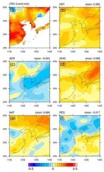
Figure 4.
The linear trends in the JJA-mean TAS (K decade−1) for P1 (1911–1940) from (a) the CRU data, (b) HST, (c) AER, (d) GHG, and (e) NAT runs, and the corresponding (f) RES. The dotted area indicates that the TAS trends are statistically significant at the 10% level. The domain average value is shown in the right corner.
The surface downwelling radiation budget is analyzed to elucidate the role of radiative forcing on TAS. It must be noted that TAS is shaped not only by radiative forcing but also feedback within the climate system that involves circulation changes that accompany temperature advection. Despite their importance, the contribution from the climate feedback cannot be analyzed in this study due to the lack of suitable data. In the early 20th century period (P1), changes in the total aerosol optical thickness (contour line in Figure 5b) is small, resulting in weak SW trends in the clear-sky condition (Figure 5b, shading). This is consistent with the result that the TAS trend by anthropogenic aerosols is almost negligible in P1. Much of the SW radiation trends (shading in Figure 5c) occur under cloudy sky conditions in close negative correlation with the changes in cloudiness (contour line in Figure 5c). The land-mean SW trend in the four runs show that the positive SW trend by the natural variability (NAT) is over ridden by the negative SW trend by anthropogenic aerosols (AER) and greenhouse gases (GHG) in Table 3. In conjunction with the increase in cloudiness (Table 4), the SW trend in HST becomes negative, i.e., the SW budget works to cool TAS. The cooling effects of the SW budget is compensated by large positive effects of the LW budget to contribute to the positive TAS trend in HST during P1. It is difficult to disseminate the LW trend in Table 3 into the one due to the forcing by each element and the one due to the feedback through the climate system. However, the large LW trend in GHG in the clear-sky condition suggests that much of the positive LW trend in HST can be assumed as an indicator of the atmospheric greenhouse effect as experienced at the surface [52,53,54,55,56], and thus a forcing towards the positive TAS trend in P1. Table 3 also shows that the SW trend in the cloudy-sky condition exceeds that in the clear-sky condition. In conjunction with the large positive cloudiness trend in P1 (Table 4), the negative SW trend in HST is strongly affected by the increase in cloudiness.
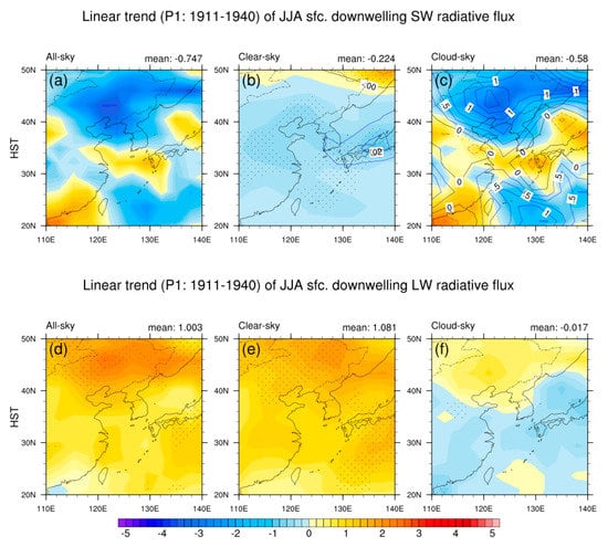
Figure 5.
The linear trends of the JJA mean downwelling SW (upper panel, shading) and LW (bottom panel, shading) radiative flux at the surface (Wm−2 decade−1, positive downward) according to cloud condition in the early 20th century (1911–1940); (a,d) all-sky; (b,e) clear-sky with total aerosol optical depth trend (contour in upper panel, positive solid line); (c,f) cloudy-sky with total cloud fraction trend (contour in upper panel) in HST. The dotted areas indicate that the trends are statistically significant at 10% level. The domain average has been shown in the right corner.
Table 3.
The land-mean linear trend (Wm−2 decade−1) of the JJA-mean downwelling SW, LW, and the net radiation at the surface from the HST, AER, GHG, and NAT simulations for P1. The numbers in the parenthesis are the corresponding values for the clear-sky and cloudy-sky condition.
Table 4.
The land-mean linear trend of the JJA-mean cloudiness from the HST, AER, GHG and NAT simulations.
3.2.2. TAS Variations in P2
The temperature variations over EA in the second period (P2) are characterized by a notable cooling trend (Figure 1c). The linear trends of TAS in each simulation show that the observed cooling in EA during P2 is a consequence of the combined cooling effects of anthropogenic aerosols and the natural forcing that exceeding the combined warming effects of the GHGs increases and the interactions (Figure 1c). The strong negative TAS trend in the CRU data occurs in southern and northeastern China, and Mongolia, with positive trends in eastern China, Taiwan and Japan (Figure 6a). The TAS trend in HST is weaker than the TAS trend from the CRU data (Figure 1c, Figure 6b). These negative TAS trend closely coincides with the TAS response to the anthropogenic aerosols and the natural forcing (Figure 6c,e). The negative TAS trends by the natural forcing (Figure 1c, Figure 6e) is due to the strong volcanic eruptions (Mount Agung 1963, Mount Awu 1966 in Figure 3b) and associated cooling in the late P2 period. The TAS trends from the single-forcing simulations in Figure 1c are consistent with the historical variations of the CO2 emissions and the variations of AODs (Figure 2) characterized by rapid increases in the CO2 concentration and anthropogenic sulfate from the 1950s. Increases in anthropogenic sulfur dioxide emissions are closely related to the increase in the total AOD over EA in P2 and P3 (Figure 2). The TAS trend in the three single-forcing simulations show that the anthropogenic aerosols (Figure 6c) and the natural forcing (Figure 6e) are the most dominant contributors to the negative TAS trend (Figure 6b), while the GHGs effects on the TAS trend are positive, mostly over the EA land surfaces (Figure 6d). The positive TAS trends over the EA land surface, mostly due to the GHG increase and the interactions, offset the cooling trends in south China, Mongolia, the coastal areas around China and Korea, and the ocean between Japan and far-eastern Russia.

Figure 6.
The linear trends in the JJA-mean TAS (K decade−1) for P2 (1941–1970) from the (a) CRU data, (b) HST, (c) AER, (d) GHG, and (e) NAT runs and (f) RES. The dotted area indicates that the TAS trends are statistically significant at 10% level. The domain average value is shown in the upper right corner.
The regional variations of the TAS trend in HST (Figure 6b) are closely related to SW variations (Figure 7a) with a spatial pattern correlation of 0.79 between the TAS trend and the SW trend. The all-sky SW trend is determined mainly in the clear-sky condition (shading in Figure 7b) and is closely correlated with the total aerosol optical depth trend (contour line in Figure 7b); however, unlike in P1, SW reduction occurs more clearly in the clear-sky condition than in the cloudy-sky condition; i.e., the direct radiative forcing by the rapidly increasing SO2 emissions and the associated increase in sulfate aerosols has played an important role in the overall cooling trend during P2. The positive SW trend in the ocean area (shading in Figure 7a,c) is due to the decrease in total cloudiness (contour line in Figure 7c). The LW trend in HST is negative over the EA region (Figure 7d), mostly under the clear sky condition (Figure 7e). This is somewhat peculiar because the GHGs concentration increases rapidly (Figure 2) and works to increase TAS (Figure 1c; Figure 7c) during P2. This will be further examined below using the land-mean LW trend in individual single-forcing simulations.
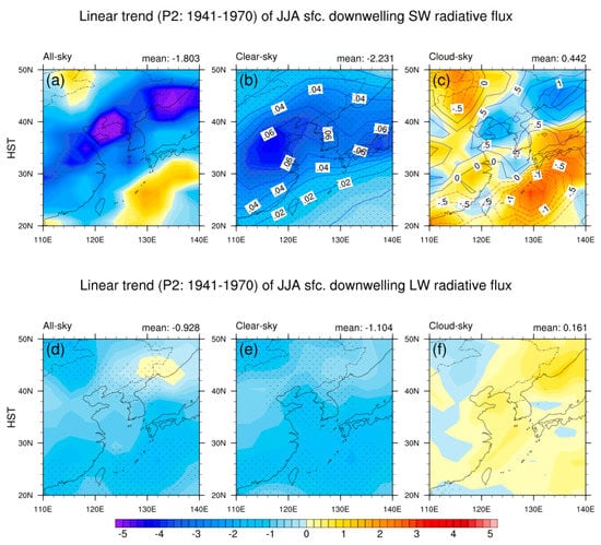
Figure 7.
The linear trends of the JJA mean downwelling SW (upper panel, shading) and LW (bottom panel, shading) radiative flux at the surface (Wm−2 decade−1, positive downward) according to cloud condition in the middle 20th century (1941–1970); (a,d) all-sky; (b,e) clear-sky with total aerosol optical depth trend (contour in upper panel, positive solid line); (c,f) cloudy-sky with total cloud fraction trend (contour in upper panel) in HST. The dotted areas indicate that the trends are statistically significant at 10% level. The domain average has been shown in the right corner.
Unlike for P1 (and P3 to be discussed in the following section), the negative land-mean SW trend in HST is consistent with the TAS trend in this period. The land-mean SW and LW trends from each single forcing runs for this period (Table 5) show that AER and the NAT forcing are related to large negative SW trend while the GHG forcing provides large positive LW trend while the LW trend in AER and NAT is negative. Thus, the negative LW trend in HST largely results from the combined negative LW effects in AER and NAT dominating the positive effects of in GHG. Similar to the SW trend, the LW trend in P2 are dominated in the clear-sky conditions in all runs except the SW trend by NAT. Table 4 shows that the magnitude of the land-mean cloudiness trend in HST is smallest in P2 among the three periods and that the natural forcing yields large positive cloudiness trend.
Table 5.
The land-mean linear trend (Wm−2 decade−1) of the JJA-mean downwelling SW, LW, and the net radiation at the surface from the HST, AER, GHG, and NAT simulations for P2. The numbers in the parenthesis are the corresponding values for the clear-sky and cloudy-sky condition.
3.2.3. TAS Variations in P3
For P3, HST shows positive TAS trend of a similarly in magnitude as in the CRU data over the EA land surface (Figure 1c). The TAS trend in GHG continues to increase (red line in Figure 1b) in response to the the rapid increase of carbon dioxide concentration (Figure 2) in the second half of the 20th century. Unlike in GHG, the negative TAS trend in AER has slowed since the mid-1980s (blue line in Figure 1b,c). Nevertheless, the negative TAS trends by anthropogenic aerosols is the only measurable offset for the positive TAS trend due to the GHGs effect (Figure 1c). Natural forcing also exerts negative TAS trend; however, its effects on the TAS trend in P3 are within the range of the uncertainty associated with the internal variability, and are insignificant compared to the effects of GHGs and anthropogenic aerosols. The weak effects of natural forcing are due to the absence of strong volcanic eruption (except Pinatubo 1991) during late 20th century (Figure 3b). It is found that much of the cooling trend due to natural forcing has been recovered since 1991 in the TAS time series for EA as well as for the entire globe (green line in Figure 1a,b). This result is consistent with the satellite-based estimates of solar irradiance changes (−0.1 to +0.1 Wm−2) associated with volcanic eruption from 1980 to 2010 [5].
The warming trend in the CRU data occurs in most of the EA region, particularly in northern EA including Mongolia, the Manchuria, the Korean Peninsula, and Japan (Figure 8a), with cooling trends in central China. The warming in HST also shows strong positive TAS trend of a similarly in magnitude and spatial pattern as in the CRU data (Figure 8b). The positive TAS trend is mostly due to GHGs increases (Figure 8d) with partial effects of the interaction over northeastern China, far-eastern Russia, and Western North Pacific (WNP) (Figure 8f). The negative TAS trend in central China closely coincides with the TAS response to the anthropogenic aerosols (Figure 8c). The anthropogenic aerosols exert significant decreasing TAS trends in central China, northern Korea, the South China Sea, and the WNP. The natural forcing (Figure 8e) yields weak decreasing TAS trend within the domain. The negative TAS trends from anthropogenic aerosols and natural forcing works to offset the warming trend due to the GHGs and interaction term in the late 20th century as noticed in the land-mean temperature trend (Figure 1c).
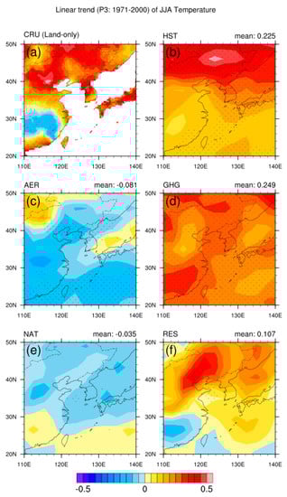
Figure 8.
The linear trends of the JJA-mean TAS (K decade−1) for P3 (1971–2000) with (a) CRU observation, (b) all-forcings, (c) anthropogenic aerosols-forcing only, (d) GHG-forcing only, and (e) natural-forcing only, (f) the residual (nonlinear interaction) term. The dotted area indicate that the TAS trends are statistically significant at 10% level. The domain average has been shown in the right corner.
Like in P2, the negative SW trend (Figure 9a) occurs largely in the clear-sky condition (shading in Figure 9b), and is closely correlated with the total AOD trend (contour line in Figure 9b). The AOD trend is positive in the domain except Japan (contour in Figure 9b), contributing to the negative clear-sky SW trend along the heavily industrialized east coast region of China (shading in Figure 9b). Reduced cloudiness in Mongolia, South Korea, and the Far-east Russia (contour red dotted line in Figure 9c) locally contributes to positive SW trends (Figure 9c, shading). Thus, the rapid increase in anthropogenic aerosols affect TAS mostly through aerosol direct effects in this period. The LW trend is positive (Figure 9d) and is mostly in the clear-sky condition (Figure 9e). Like in P1 and P2, the geographical variations of the TAS trend in HST closely resemble the LW trend in the clear-sky condition (Figure 9d).

Figure 9.
The linear trends of the JJA mean downwelling SW (upper panel, shading) and LW (bottom panel, shading) radiative flux at the surface (Wm−2 decade−1, positive downward) according to cloud condition in the late 20th century (1971–2000); (a,d) all-sky; (b,e) clear-sky with total aerosol optical depth trend (contour in upper panel, positive solid line); (c,f) cloudy-sky with total cloud fraction trend (contour in upper panel) in HST. The dotted areas indicate that the trends are statistically significant at 10% level. The domain average has been shown in the right corner.
The land-mean SW and LW trends during P3 are similar to those in P1 as shown in the trends in individual simulations (Table 6). For example, despite the positive TAS trend in HST, the SW trend is negative. The leading terms for the SW and LW trend are the negative trend in AER and the positive trend in GHG, respectively. Thus, the effects of negative SW of anthropogenic aerosols is overcome by the positive effects of GHG increases to contribute to the positive TAS trend in P3. Table 4 shows that the feedback through clouds in P3 may be smaller than that in P1 although it is larger than in P2.
Table 6.
The land-mean linear trend (Wm−2 decade−1) of the JJA-mean downwelling SW, LW, and the net radiation at the surface from the HST, AER, GHG, and NAT simulations for P3. The numbers in the parenthesis are the corresponding values for the clear-sky and cloudy-sky condition.
3.2.4. Effects of Interactions among Individual Forcing Elements
The residual term RES in (2) arises from the feedback among the forcings by greenhouse gases, aerosols, and natural variability that cannot be estimated in single-forcing experiments. As shown in Figure 1c, the feedback among these forcings to the climate system is also important in determining the TAS trend. According to Feichter et al. [23], the feedback through the atmospheric hydrologic cycle plays an important role in shaping the nonlinear aspect of the climate response to GHGs and aerosol forcings. Because it is practically impossible to isolate individual feedback processes in climate model simulations, we attempt to estimate the effects of the interaction term relative to the sum of the effects from the single forcing simulations. The interaction term in P1, the early 20th century period, is of smaller/larger magnitude/uncertainty compared to the sum of the effects from all single-forcing runs. Since the mid-20th century, the effects of the interaction term in the TAS trend become more obvious with much smaller uncertainty compared to that in P1 (Figure 1c). To identify plausible processes involved in the interaction term, we compare the linear trends of hydrological variables (such as water vapor, cloudiness, and precipitation rate etc.) in the all-forcing runs (HST) against those in the sum of single-forcing simulations (Figure 10):
SUMS = AER + GHG + NAT
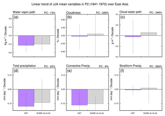
Figure 10.
The linear trends of the JJA-mean variables; (a) water vapor path; (b) total cloud fraction; (c) cloud water path; (d) total precipitation rate; (e) convective precipitation rate; (f) stratiform precipitation rate; in combined all-forcing runs (HST; purple bar) and the sum of single-forcing simulations (anthropogenic aerosol, GHGs, and natural forcing; gray bar) for P2 (1941–1970) over East Asia (20°–50° N and 110°–140° E). Error bars indicate the standard deviation of CMIP5 models MME. The percentage change PC in % {(HST-SUMS)/|HST|} has been shown in the right corner.
Examinations of the water vapor path, cloudiness, cloud-water path, and precipitation show that the interaction term works to decrease the atmospheric water vapor and cloud water contents and cloudiness as well as precipitation in P2 (Figure 10). The decreasing trend in the condensed phase of hydrometeors, cloud water (−346% of HST) and precipitation (−22% of HST), is much larger than in water vapor (−13% of HST). The reduced atmospheric water vapor, in turn, decreases condensation to enhance the negative trends in the cloud water path and precipitation (Figure 10c,d). The negative trend in the total precipitation in HST is mainly by decreased convective cloud (Figure 10e), whereas the stratiform precipitation trend is almost negligible in P2 (purple in Figure 10f). The large decrease in cloudiness and cloud water path (Figure 10b,c) by the interaction term suggests that the decreased water vapor path results in suppressing both convective precipitation (−9% of HST) and stratiform precipitation (−280% of HST) (Figure 10e,f); however, the amount of stratiform precipitation is much smaller than the amount of convective precipitation.
In P3, the interaction term contributes to the increase in atmospheric water vapor, cloud water contents, and precipitation, but exerts minimal effects on cloudiness (Figure 11a–d). The increase in the condensed phase of hydrometeors, cloud water (46% of HST) and precipitation (88% of HST), is much larger than in water vapor (24% of HST). The enhanced atmospheric water vapor, in turn, increases condensation to enhance the positive trends in cloud water path (Figure 11c) and precipitation (Figure 11d). Like in P2, the positive trend in the total precipitation in HST is determined mainly by the convective cloud precipitation (Figure 11e); unlike in P2, the interaction term contribute to the large increase in convective precipitation (133% of HST). The slight decrease (almost negligible, −3% of HST) in cloudiness by the interaction term (Figure 11b) suggests that the increased water vapor and cloud water contents by the interaction term largely result in enhancing deep clouds than stratiform clouds (−133% of HST). (Figure 11e,f). Note that the descriptions on the effects of the interaction term here are largely qualitative. Legitimate quantitative analyses are not feasible because of the complexity in the feedbacks and also because it requires much more data that are available from the CMIP5 archive.
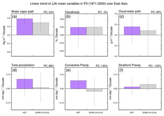
Figure 11.
The linear trends of the JJA-mean variables; (a) water vapor path; (b) total cloud fraction; (c) cloud water path; (d) total precipitation rate; (e) convective precipitation rate; (f) stratiform precipitation rate; in combined all-forcing runs (HST; purple bar) and the sum of single-forcing simulations (anthropogenic aerosol, GHGs, and natural forcing; gray bar) for P3 (1971–2000) over East Asia (20°–50° N and 110°–140° E). Error bars indicate the standard deviation of CMIP5 models MME. The percentage change PC in % {(HST-SUMS)/|HST|} has been shown in the right corner.
4. Summary and Discussion
The relationships between the multi-decadal variations of the summer-mean TAS and the emissions of anthropogenic GHGs, aerosols, and natural agents over the EA land surface in the 20th century are examined using six-member CMIP5 GCM ensembles from five sensitivity simulations in which various combinations of the historical variations of GHGs, anthropogenic aerosol emissions, and the natural variability are implemented. Unlike most previous studies that explore these effects for an equilibrium state [23,34], we attempt to understand the relationship between the historical TAS variation and these external forcing more realistically from transient simulations. We also examined the effects of the internal variability on the summer TAS over EA using the simulations in which GHG concentrations and anthropogenic aerosol emissions are fixed at the pre-20th century level (INT). For the analysis period, both observed and simulated summer TAS trends are mostly stronger than the magnitude of internal variability, suggesting that the observed summer TAS variations are primarily induced by anthropogenic and natural forcing with minimal effects from the internal variability.
The CRU data shows that the 20th century TAS variations are characterized by warming trends for the early (1901–1940) and late (1971–2000) 20th century periods with a period of cooling trend between them (1941–1970). The six-member HST-run ensemble that includes the historical variations of GHG concentrations, anthropogenic aerosol emissions, and natural forcings by solar and volcanic activities, simulates reasonably well the observed variations of the land-mean summer TAS during the 20th century for EA as well as for the entire globe.
Three single-forcing simulations are performed to calculate separately the effects of GHGs, anthropogenic aerosol emissions, and natural forcing on the TAS variations. The effects of interactions between these external forcings on TAS are estimated as the residual term between HST and the sum of the single-forcing runs. Analyses of the simulated data show that the TAS trend in the three periods can be related to distinct effects of the variations in the anthropogenic (GHGs and aerosols) and natural (solar and volcanoes) forcings, as well as their interactions, within the corresponding period. The main results from the analysis of the experiments include:
- For P1, the positive TAS trend over the EA land surface is primarily due to the increase GHGs and natural variability. The warming trend by the natural variability is mainly by the long-tem recovery of TAS from the large volcanic activities in late 19th/early 20th century that lasted until 1940. The positive effect of the solar activity is much smaller than the long-term recovery from the volcanic activities. Emissions of anthropogenic aerosols and the interaction term exert little impacts on the TAS trend in the early 20th century period.
- The negative TAS trend over EA in P2, 1941–1970, results from the combined cooling effect of the increased anthropogenic aerosols and natural forcing as they exceed the combined warming effect of the increased GHG concentration and the interaction term. The anthropogenic aerosol effects in P2 are mainly shaped by the increase in the total aerosol optical depth. The natural forcing effects are due to strong volcanic eruptions during the late P2 period.
- For P3, the increase in GHGs mainly contributes to the positive TAS trend. The aerosol effects on SW occur mainly in the clear-sky condition. Thus, aerosol direct effects appear to be critical in shaping the aerosol effects on TAS over EA. However, the effects of negative SW of anthropogenic aerosols is overcome by the positive effects of GHG increases to contribute to the positive TAS trend in the late 20th century period.
- For P1 and P3, the surface SW forcing is not the driving force behind the TAS change in HST as the results show that the warming effects of the surface LW forcing dominate the cooling effects of the surface SW forcing. Further details of the relationship between the LW forcing and TAS cannot be analyzed because the LW forcing to TAS cannot be separated from the LW response to TAS using the data available to us.
- It is noticed that the nonlinear interaction effect between the anthropogenic and natural agents substantially contributes to the TAS variations since the mid-20th century (in P2 and P3). The interaction term also contributes to the hydrological variables. The decreased (increased) water vapor and cloud water contents by the interaction term result in the suppression (enhancement) of convective precipitation in P2 (P3).
- Surface downwelling LW flux is well correlated with the changes in TAS in all experiments and for all time periods. In fact, for P1 and P3, the positive effects of the downwelling LW exceed the negative effects of downwelling SW to contribute to the positive TAS trend in the corresponding period. Quantification of the effects of LW on the TAS trend is not feasible because the simulated LW trends represent the combined effects of the LW forcing and the LW response to the altered TAS.
This study is among the few climate modeling studies that explored the effects of the forcing by natural elements, aerosols, and GHGs in East Asia within a transient framework. The CMIP5 GCM simulations analyzed appears to successfully reproduce the historical TAS in the 20th century and attribute key multi-decadal variability to the historical emissions of GHGs, anthropogenic aerosols, and natural agents, albeit qualitatively. Results in this study are consistent with the previous study [35] that demonstrated that the positive TAS trend in the late 20th century was mostly due to GHG increases, although it was offset significantly by the cooling due to anthropogenic aerosols and the effect of natural forcing was insignificant. However, this study finds that in detail the main forcings on the TAS trends over EA are not uniform but vary according to the analysis periods. In addition, it is also found that the nonlinear interaction among the anthropogenic GHG, aerosols, and natural forcing becomes considerably important in shaping the historical TAS since mid-20th century. Analyses of the effects of the interaction term on the fields related to the atmospheric water cycle suggest that the interaction term affects TAS largely by modifying atmospheric hydrometeors. Detailed mechanisms involved in the interaction term need further research but are beyond the scope of this study. Despite the success, the limitations of this study should be noted. We adopted CMIP5 multi model ensemble analysis to understand the impact of individual forcings on TAS and their uncertainties. However, the interaction term can still be affected by the differences in the specific components of climate forcing and cloud microphysics used among the CMIP5 models. In particular, the uncertainties can be large due to the differences in the physical processes associated with aerosol and cloud interactions among CMIP5 models. Another caveat of this study is the lack of the analysis of the cloud fields, especially the vertical profiles of cloud optical properties. Analyses of the cloud-related fields require special sampling of model fields that is not included in the CMIP5 designs. Uncertainties in attributing the TAS change to forcing terms also arise from our inability to analyze other key forcing terms such as the contribution of the temperature advection related to the altered large-scale circulation because we could not obtain the model data for these analyses. These shortcomings in this study will be explored in future studies.
Supplementary Materials
The following are available online at https://www.mdpi.com/2073-4433/10/11/690/s1, Table S1: The forcing agents in CMIP5 models (BC: black carbon, OC: organic carbon, CAE: cloud albedo effect, CLE: cloud lifetime effect, DS: dust, VI: volcanic, SS: sea-salt, LU: land use, SI: solar activity). Strikethrough indicates the component is not considered.
Author Contributions
S.S. wrote the manuscript text and contributed to the graphics. J.K., S.S.Y., H.L., K.-O.B., and Y.-H.B. contributed to the methods, results, analysis, discussion, and revision of the manuscript.
Funding
This research was funded by National Institute of Meteorological Sciences grant number: 1365003000 and by Korea Meteorological Administration grant number: KMI2018-03511.
Conflicts of Interest
The authors declare no conflicts of interest.
References
- Santer, B.D.; Taylor, K.E.; Wigley, T.M.L.; Penner, J.E.; Jones, P.D.; Kubasch, U. Towards the detection and attribution of an anthropogenic effect on climate. Clim. Dyn. 1995, 12, 79–100. [Google Scholar] [CrossRef]
- Hansen, J.; Sato, M.; Ruedy, R.; Lacis, A.; Oinas, V. Global warming in the twenty-first century: An alternative scenario. Proc. Natl. Acad. Sci. USA 2000, 97, 9875–9880. [Google Scholar] [CrossRef]
- Ramanathan, V.; Crutzen, P.J.; Kiehl, J.T.; Rosenfeld, D. Aerosols, climate, and the hydrological cycle. Science 2001, 294, 2119–2124. [Google Scholar] [CrossRef] [PubMed]
- Dufresne, J.L.; Quaas, J.; Boucher, O.; Denvil, S.; Fairhead, L. Contrast in the effects on climate of anthropogenic sulfate aerosols between the 20th and the 21st century. Geophys. Res. Lett. 2005, 32. [Google Scholar] [CrossRef]
- IPCC. Climate Change 2014: Anthropogenic and Natural Radiative Forcing. In Contribution of Working Group I to the Fifth Assessment Report of the Intergovernmental Panel on Climate Change; Cambridge University Press: Cambridge, UK; New York, NY, USA, 2014; pp. 659–740. [Google Scholar]
- Wilcox, L.J.; Highwood, E.J.; Dunstone, N.J. The influence of anthropogenic aerosol on multi-decadal variations of historical global climate. Environ. Res. Lett. 2013, 8, 024033. [Google Scholar] [CrossRef]
- IPCC. Climate Change 2014: Synthesis Report. In Contribution of Working Group I, II, and III to the Fifth Assessment Report of the Intergovernmental Panel on Climate Change; Cambridge University Press: Cambridge, UK; New York, NY, USA, 2014; pp. 1–151. [Google Scholar]
- Park, C.; Jeong, S.; Ho, C.; Kim, J. Regional variations in potential plant habitat changes in response to multiple global warming scenarios. J. Clim. 2015, 28, 2884–2899. [Google Scholar] [CrossRef]
- IPCC. Climate Change 2007: Synthesis Report. In Contribution of Working Group I, II, and III to the Fourth Assessment Report of the Intergovernmental Panel on Climate Change; Cambridge University Press: Cambridge, UK; New York, NY, USA, 2007; pp. 1–103. [Google Scholar]
- IPCC. Climate Change 2007: Changes in Atmospheric Constituents and in Radiative Forcing. In Contribution of Working Group I to the Fifth Assessment Report of the Intergovernmental Panel on Climate Change; Cambridge University Press: Cambridge, UK; New York, NY, USA, 2007; pp. 131–234. [Google Scholar]
- Menon, S.; Hansen, J.; Nazarenko, L.; Luo, Y. Climate effects of black carbon aerosols in China and India. Science 2002, 297, 2250–2253. [Google Scholar] [CrossRef]
- Mitchell, J.; Johns, T.; Gregory, J.; Tett, S. Climate response to increasing levels of greenhouse gases and sulfate aerosols. Nature 1995, 376, 501–504. [Google Scholar] [CrossRef]
- Lohmann, U.; Feichter, J.; Penner, J.; Leaitch, R. Indirect effect of sulfate and carbonaceous aerosols: A mechanistic treatment. J. Geophys. Res. 2000, 105, 12193–12206. [Google Scholar] [CrossRef]
- Jones, A.; Roberts, D.L.; Woodage, M.J.; Johnson, C.E. Indirect sulphate aerosol forcing in a climate model with an interactive sulphur cycle. J. Geophys. Res. 2001, 106, 20293–20310. [Google Scholar] [CrossRef]
- Chuang, C.C.; Penner, J.E.; Prospero, J.M.; Grant, K.E.; Rau, G.H.; Kawamoto, K. Cloud susceptibility and the first aerosol indirect forcing: Sensitivity to black carbon and aerosol concentration. J. Geophys. Res. 2002, 107, 4564. [Google Scholar] [CrossRef]
- Quaas, J.; Boucher, O. Constraining the first aerosol indirect radiative forcing in the LMDZ GCM using POLDER and MODIS satellite data. Geophys. Res. Lett. 2005, 32. [Google Scholar] [CrossRef]
- Kim, J.; Gu, Y.; Liou, K.N. The impact of aerosol radiative forcing on surface insolation and spring snowmelt in the southern Sierra Nevada. J. Hydrometeorol. 2006, 7, 976–983. [Google Scholar] [CrossRef]
- Kim, J.; Gu, Y.; Liou, K.N.; Park, R.; Song, C. Direct and semi-direct radiative effects of anthropogenic aerosols in the western United States: Seasonal and geographical variations according to regional climate characteristics. Clim. Chang. 2012, 111, 859–877. [Google Scholar] [CrossRef]
- Giorgi, F.; Bi, X.; Qian, Y. Direct radiative forcing and regional climate effects of anthropogenic aerosols over East Asia: A regional coupled climate-chemistry/aerosol model study. J. Geophy. Res. 2002, 107. [Google Scholar] [CrossRef]
- Massie, S.T.; Torres, O.; Smith, S.J. Total ozone mapping spectrometer (TOMS) observations of increase in Asian aerosol in winter from 1979 to 2000. J. Geophys. Res. 2004, 109. [Google Scholar] [CrossRef]
- Remer, L.A.; Kleidman, R.G.; Levy, R.C.; Kaufman, Y.J.; Tanre, D.; Matto, S.; Martins, J.V.; Ichoku, C.; Koren, I.; Yu, H.; et al. Global aerosol climatology from the MODIS satellite sensors. J. Geophys. Res. 2008, 113. [Google Scholar] [CrossRef]
- Kaufman, Y.J.; Tanre, D.; Boucher, O. A satellite view of aerosols in the climate system. Nature 2002, 419, 215–223. [Google Scholar] [CrossRef]
- Feichter, J.; Roeckner, E.; Lohmann, U.; Liepert, B. Nonlinear aspects of the climate response to greenhouse gas and aerosol forcing. J. Clim. 2004, 17, 2384–2398. [Google Scholar] [CrossRef]
- Lau, K.M.; Kim, M.K.; Kim, K.M. Asian summer monsoon anomalies induced by aerosol direct forcing: The role of the Tibetan Plateau. Clim. Dyn. 2006, 26, 855–864. [Google Scholar] [CrossRef]
- Lau, K.M.; Kim, K.M. Observational relationships between aerosol and Asian monsoon rainfall, and circulation. Geophys. Res. Lett. 2006, 33. [Google Scholar] [CrossRef]
- Huang, Y.; Chameides, W.L.; Dickinson, R.E. Direct and indirect effects of anthropogenic aerosols on regional precipitation over East Asia. J. Geophys. Res. 2007, 112. [Google Scholar] [CrossRef]
- Liu, Y.; Sun, J.; Yang, B. The effects of black carbon and sulphate aerosols in China regions on East Asia monsoons. Tellus B 2009, 61, 642–656. [Google Scholar] [CrossRef]
- Zhang, H.; Wang, Z.; Wang, Z.; Liu, Q.; Gong, S.; Zhang, X.; Shen, Z.; Lu, P.; Wei, X.; Che, H.; et al. Simulation of direct radiative forcing of aerosols and their effects on East Asian climate using an interactive AGCM-aerosol coupled system. Clim. Dyn. 2012, 38, 1675–1693. [Google Scholar] [CrossRef]
- Guo, L.; Highwood, E.J.; Shaffrev, L.C.; Turner, A.G. The effect of regional changes in anthropogenic aerosols on rainfall of the East Asian summer monsoon. Atmos. Chem. Phys. 2013, 13, 1521–1534. [Google Scholar] [CrossRef]
- Jiang, Y.; Liu, X.; Yang, X.Q.; Wang, M. A numerical study of the effect of different aerosol types on East Asian summer clouds and precipitation. Atmos. Environ. 2013, 70, 51–63. [Google Scholar] [CrossRef]
- Wu, L.; Su, H.; Jiang, J.H. Regional simulation of aerosol impacts on precipitation during the East Asian summer monsoon. J. Geophys. Res. 2013, 118, 6454–6467. [Google Scholar] [CrossRef]
- Li, Z.; Lau, W.K.-M.; Ramanathan, V.; Wu, G.; Ding, Y.; Manoj, M.G.; Liu, J.; Qian, Y.; Li, J.; Zhou, T.; et al. Aerosol and monsoon climate interaction over Asia. Rev. Geophys. 2016, 54, 866–929. [Google Scholar] [CrossRef]
- Hansen, J.; Nazarenko, L.; Ruedy, R.; Sato, M.; Willis, J.; Genio, A.D.; Koch, D.; Lacis, A.; Lo, K.; Menon, S.; et al. Earth’s energy imbalance: Confirmation and implications. Science 2005, 308, 1431–1435. [Google Scholar] [CrossRef]
- Kritjansson, J.; Iverson, T.; Kirkevag, A.; Seland, O. Responses of the climate system to aerosol direct and indirect forcing: Role of cloud feedbacks. J. Geophys. Res. 2005, 110. [Google Scholar] [CrossRef]
- Song, F.; Zhou, T.; Qian, Y. Responses of East Asian summer monsoon to natural and anthropogenic forcings in the 17 latest CMIP5 models. Geophys. Res. Lett. 2014, 41, 596–603. [Google Scholar] [CrossRef]
- Taylor, K.E.; Stouffer, R.J.; Meehl, G.A. An overview of CMIP5 and the experiment design. Bull. Am. Meteorol. Soc. 2012, 93, 485–498. [Google Scholar] [CrossRef]
- Chylek, P.; Li, J.; Dubey, M.K.; Wang, M.; Lesins, G. Observed and model simulated 20th century Arctic temperature variability: Canadian Earth System Model CanESM2. Atmos. Chem. Phys. Discuss. 2011, 11, 22893–22907. [Google Scholar] [CrossRef]
- Jeffrey, S.J.; Rotstayn, L.; Collier, M.A.; Dravitzki, S.M.; Hamalainen, C.; Moeseneder, C.; Wong, K.K.; Syktus, J.I. Australia’s CMIP5 submission using the CSIRO-Mk3.6 model. Aust. Meteorol. Oceanogr. J. 2013, 63, 1–13. [Google Scholar] [CrossRef]
- Griffies, S.M.; Winton, M.; Donner, L.; Horowitz, L.W.; Downes, S.M.; Farneti, R.; Gnanadesikan, A.; Hurlin, J.; Lee, H.-C.; Liang, Z.; et al. The GFDL CM3 Coupled Climate Model: Characteristics of the Ocean and Sea Ice simulations. J. Clim. 2011, 24, 3520–3544. [Google Scholar] [CrossRef]
- Dunne, J.P.; John, J.G.; Adcroft, A.J.; Griffies, S.M.; Hallberg, R.W.; Shevliakova, E.; Stouffer, R.J.; Cooke, W.; Dunne, K.A.; Harrison, M.J.; et al. GFDL’s ESM2 Global Coupled Climate-Carbon Earth System Models. Part I: Physical Formulation and Baseline Simulation Characteristics. J. Clim. 2012, 25, 6646–6665. [Google Scholar] [CrossRef]
- Dufresne, J.-L.; Foujols, M.-A.; Denvil, S.; Caubel, A.; Marti, O.; Aumont, O.; Balkanski, Y.; Bekki, S.; Bellenger, H.; Benshila, R.; et al. Climate change projections using the IPSL-CM5 Earth System Model: From CMIP3 to CMIP5. Clim. Dyn. 2015, 40, 2123–2165. [Google Scholar] [CrossRef]
- Bentsen, M.; Bethke, I.; Debernard, J.B.; Iversen, T.; Kirkevag, A.; Seland, O.; Drange, H.; Roelandt, C.; Seierstad, I.A.; Hoose, C.; et al. The Norwegian Earth System Model, NorESM1-M—Part 1: Description and basic evaluation of the physical climate. Geosci. Model. Dev. 2013, 6, 687–720. [Google Scholar] [CrossRef]
- Harris, I.; Jones, P.D.; Osborn, T.J.; Lister, D.H. Updated high-resolution grids of monthly climatic observations—The CRU T3.10 Dataset. Int. J. Climatol. 2014, 34, 623–642. [Google Scholar] [CrossRef]
- Lean, J. Evolution of the sun’s spectral irradiance since the maunder minimum. Geophys. Res. Lett. 2000, 27, 2425–2428. [Google Scholar] [CrossRef]
- Lean, J.; Beer, J.; Bradley, R. Reconstruction of solar irradiance since 1610: Implications for climate change. Geophys. Res. Lett. 1995, 22, 3195–3198. [Google Scholar] [CrossRef]
- Cliver, E.W.; Clette, F.; Svalgaard, L. Recalibrating the sunspot number (SSN): The SSN Workshop. Cent. Eur. Astrophys. Bull. 2013, 37, 401–416. [Google Scholar]
- Sato, M.; Hansen, J.E.; McCormick, M.P.; Pollack, J.B. Stratospheric aerosol optical depths, 1850–1990. J. Geophys. Res. 1993, 98, 22987–22994. [Google Scholar] [CrossRef]
- Bourassa, A.E.; Robock, A.; Randel, W.J.; Deshler, T.; Rieger, L.A.; Lloyd, N.D.; Llewellyn, E.J.; Degenstein, D.A. Large volcanic aerosol load in the stratosphere linked to Asian monsoon transport. Science 2012, 337. [Google Scholar] [CrossRef] [PubMed]
- Shiogama, H.; Nagashima, T.; Yokohata, T.; Crooks, S.A.; Nozawa, T. Influence of volcanic activity and changes in solar irradiance on surface air temperatures in the early twentieth century. Geophys. Res. Lett. 2006, 33. [Google Scholar] [CrossRef]
- Moss, R.H.; Nakicenovic, N.; O’Neil, B.C. Towards New Scenarios for Analysis of Emissions, Climate Change, Impacts, and Response Strategies; IPCC: Geneva, Switzerland, 2008; ISBN 978-92-9169-125-8. [Google Scholar]
- RCP Database. Available online: http://www.iiasa.ac.at/web-apps/tnt/RcpDb (accessed on 1 March 2019).
- Wild, M.; Folini, D.; Schar, C.; Loeb, N.; Dutton, E.G.; Konig-Langlo, G. The global energy balance from a surface perspective. Clim. Dyn. 2013, 40, 3107–3134. [Google Scholar] [CrossRef]
- Wild, M.; Ohmura, A.; Cubasch, U. GCM-Simulated Surface Energy Fluxes in Climate Change Experiments. J. Clim. 1997, 10, 3093–3110. [Google Scholar] [CrossRef]
- Marty, C.; Philipona, R.; Delamere, J.; Dutton, E.G.; Michalsky, J.; Stamnes, K.; Storvold, R.; Stoffel, T.; Clough, S.A.; Mlawer, E.J. Downward longwave irradiance uncertainty under arctic atmospheres: Measurements and modeling. J. Geophys. Res. 2003, 108. [Google Scholar] [CrossRef]
- Viudez-Mora, A.; Costa-Suros, M.; Calbo, J.; Gonzalez, J.A. Modeling atmospheric longwave radiation at the surface during overcast skies: The role of cloud base height. J. Geophys. Res. 2015, 120, 199–214. [Google Scholar] [CrossRef]
- Wang, K.; Dickinson, R.E. Global atmospheric downward longwave radiation at the surface from ground-based observations, satellite retrievals, and reanalyses. Rev. Geophys. 2013, 51, 150–185. [Google Scholar] [CrossRef]


© 2019 by the authors. Licensee MDPI, Basel, Switzerland. This article is an open access article distributed under the terms and conditions of the Creative Commons Attribution (CC BY) license (http://creativecommons.org/licenses/by/4.0/).