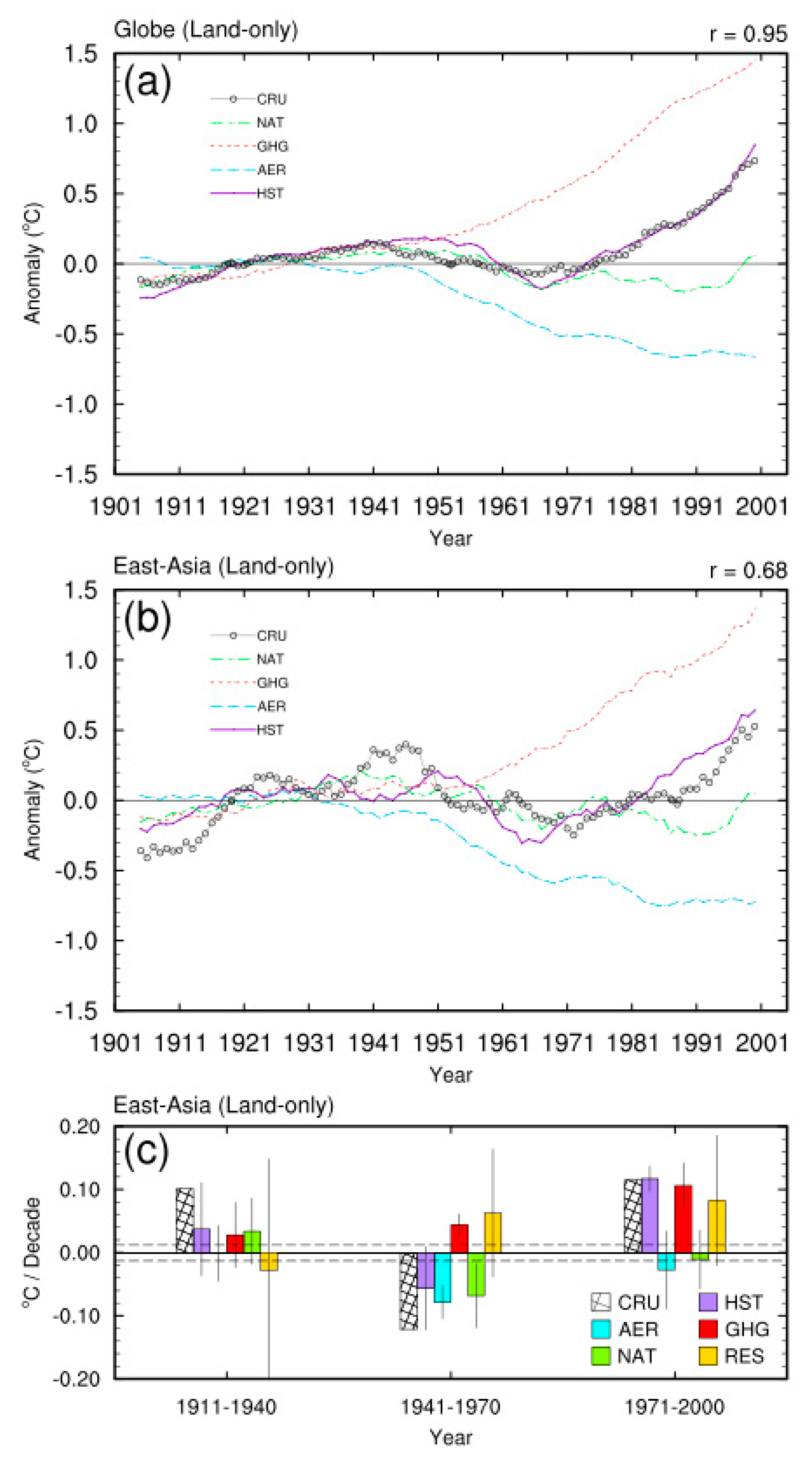
Figure 1.
The June to August (JJA)-mean surface air temperature (TAS) time series in the 20th century from Climate Research Unit (CRU) and the GCM simulations over the land surface of (
a) the entire globe and (
b) EA, and (
c) the linear trend of TAS obtained from the simulations in
Table 2 and the corresponding residuals for the three periods. In (
a) and (
b), the 10 year running-mean TAS anomaly (1901–2005) over the entire globe and EA are shown. CRU indicates the CRU data and RES is the residual term calculated from the simulations as Equation (2); abbreviations for other runs are the same as in
Table 2. Error bars indicate the standard deviation of CMIP5-model multi-model ensemble (MMEs) from each simulation. The black dashed horizontal lines indicate the range of the internal variability on the 30 year timescale estimated as one standard deviation of the 30-year trends of the 100 samples from the Pi-Control MME as described in
Section 2.
Figure 2.
The time variation of the historical emissions of anthropogenic sulphur dioxide and carbon dioxide from 1900 to 2000 based on the RCP database v2.0.5 [
51] and the simulated aerosol optical depth from CMIP5 models. The global sulphur dioxide emission (blue dashed line with open circle), the Asian emissions (blue solid line with closed circle) are shown; the black line indicate the total aerosol optical depth at 550 nm in JJA over East Asia.
Figure 3.
Time variation of (a) total solar irradiance (TSI; red solid line) for CMIP5 & observed sunspot number (blue dotted line), (b) stratospheric aerosol optical depth at 550 nm (SAOD) from 1880 to 2000. Annual mean TSI time series provided from National Oceanic and Atmospheric Administration (NOAA). Sunspot data from Solar Influences Data Analysis Center (SIDC, Royal Observatory of Belgium). Monthly mean stratospheric aerosol optical depth (SAOD) dataset used from NASA Goddard Institute for Space Studies (GISS). Dotted vertical gray lines denote the times of maximum SAOD during major volcanic eruptions.
Figure 4.
The linear trends in the JJA-mean TAS (K decade−1) for P1 (1911–1940) from (a) the CRU data, (b) HST, (c) AER, (d) GHG, and (e) NAT runs, and the corresponding (f) RES. The dotted area indicates that the TAS trends are statistically significant at the 10% level. The domain average value is shown in the right corner.
Figure 5.
The linear trends of the JJA mean downwelling SW (upper panel, shading) and LW (bottom panel, shading) radiative flux at the surface (Wm−2 decade−1, positive downward) according to cloud condition in the early 20th century (1911–1940); (a,d) all-sky; (b,e) clear-sky with total aerosol optical depth trend (contour in upper panel, positive solid line); (c,f) cloudy-sky with total cloud fraction trend (contour in upper panel) in HST. The dotted areas indicate that the trends are statistically significant at 10% level. The domain average has been shown in the right corner.
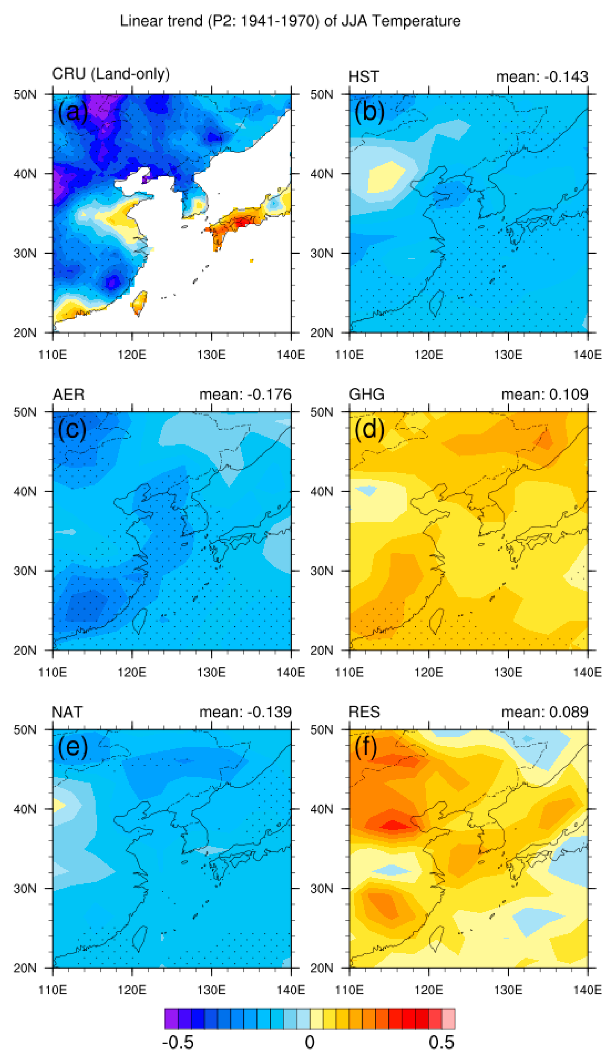
Figure 6.
The linear trends in the JJA-mean TAS (K decade−1) for P2 (1941–1970) from the (a) CRU data, (b) HST, (c) AER, (d) GHG, and (e) NAT runs and (f) RES. The dotted area indicates that the TAS trends are statistically significant at 10% level. The domain average value is shown in the upper right corner.
Figure 7.
The linear trends of the JJA mean downwelling SW (upper panel, shading) and LW (bottom panel, shading) radiative flux at the surface (Wm−2 decade−1, positive downward) according to cloud condition in the middle 20th century (1941–1970); (a,d) all-sky; (b,e) clear-sky with total aerosol optical depth trend (contour in upper panel, positive solid line); (c,f) cloudy-sky with total cloud fraction trend (contour in upper panel) in HST. The dotted areas indicate that the trends are statistically significant at 10% level. The domain average has been shown in the right corner.
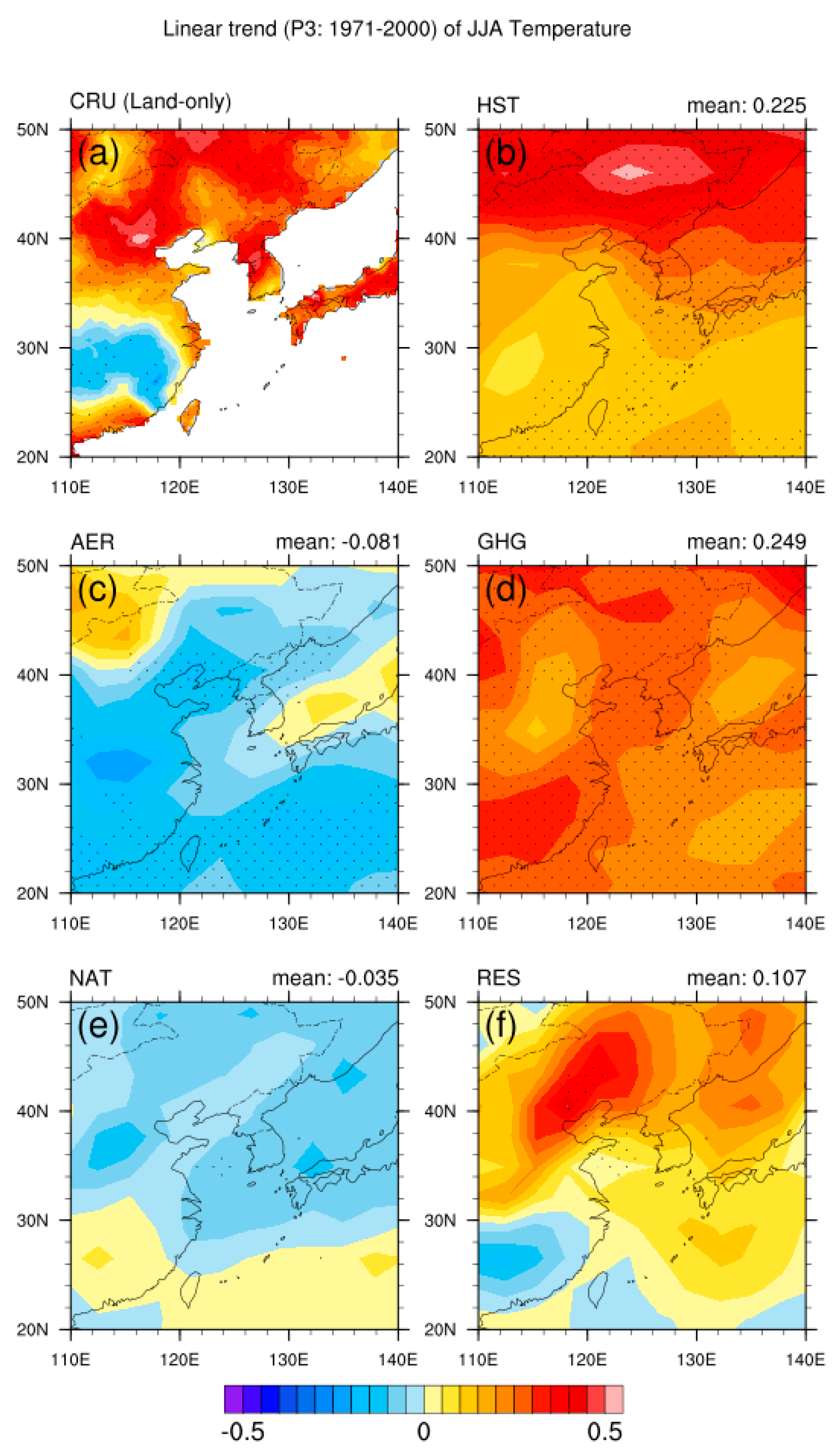
Figure 8.
The linear trends of the JJA-mean TAS (K decade−1) for P3 (1971–2000) with (a) CRU observation, (b) all-forcings, (c) anthropogenic aerosols-forcing only, (d) GHG-forcing only, and (e) natural-forcing only, (f) the residual (nonlinear interaction) term. The dotted area indicate that the TAS trends are statistically significant at 10% level. The domain average has been shown in the right corner.
Figure 9.
The linear trends of the JJA mean downwelling SW (upper panel, shading) and LW (bottom panel, shading) radiative flux at the surface (Wm−2 decade−1, positive downward) according to cloud condition in the late 20th century (1971–2000); (a,d) all-sky; (b,e) clear-sky with total aerosol optical depth trend (contour in upper panel, positive solid line); (c,f) cloudy-sky with total cloud fraction trend (contour in upper panel) in HST. The dotted areas indicate that the trends are statistically significant at 10% level. The domain average has been shown in the right corner.
Figure 10.
The linear trends of the JJA-mean variables; (a) water vapor path; (b) total cloud fraction; (c) cloud water path; (d) total precipitation rate; (e) convective precipitation rate; (f) stratiform precipitation rate; in combined all-forcing runs (HST; purple bar) and the sum of single-forcing simulations (anthropogenic aerosol, GHGs, and natural forcing; gray bar) for P2 (1941–1970) over East Asia (20°–50° N and 110°–140° E). Error bars indicate the standard deviation of CMIP5 models MME. The percentage change PC in % {(HST-SUMS)/|HST|} has been shown in the right corner.
Figure 11.
The linear trends of the JJA-mean variables; (a) water vapor path; (b) total cloud fraction; (c) cloud water path; (d) total precipitation rate; (e) convective precipitation rate; (f) stratiform precipitation rate; in combined all-forcing runs (HST; purple bar) and the sum of single-forcing simulations (anthropogenic aerosol, GHGs, and natural forcing; gray bar) for P3 (1971–2000) over East Asia (20°–50° N and 110°–140° E). Error bars indicate the standard deviation of CMIP5 models MME. The percentage change PC in % {(HST-SUMS)/|HST|} has been shown in the right corner.
Table 1.
The descriptions of the CMIP5 models used in this study.
Table 1.
The descriptions of the CMIP5 models used in this study.
| Model | Institution | Resolution |
|---|
| CanESM2 [37] | Canadian Centre for Climate Modelling and Analysis (CCCma) | 2.813° × 2.813° |
| CSIRO-Mk3.6.0 [38] | Commonwealth Scientific and Industrial Research Organisation and the Queensland Climate Change Centre of Excellence (CSIRO-QCCCE) | 1.875° × 1.875° |
| GFDL-CM3 [39] | National Oceanic and Atmospheric Administration/Geophysical Fluid Dynamics Laboratory (NOAA/GFDL) | 2.5° × 2° |
| GFDL-ESM2M [40] | Same as GFDL-CM3 (NOAA/GFDL) | 2.5° × 2° |
| IPSL-CM5A-LR [41] | Institute Pierre-Simon Laplace (IPSL) | 3.75° × 1.87° |
| NorESM1-M [42] | Norwegian Climate Centre (NCC) | 2.5° × 1.875° |
Table 2.
Five sets of climate simulations are used in this study.
Table 2.
Five sets of climate simulations are used in this study.
| Name | Information |
|---|
| HST | The twentieth century historical climate simulations (historical; all forcing runs). The forcing data are from the CMIP5 for IPCC AR5. The scenario data include natural agent change (mainly solar and volcanic) and anthropogenic agent changes (well-mixed GHGs, aerosols, ozone, land-use changes) |
| AER | Aerosols-only forcing simulations (historicalMisc runs). Note that the level of complexity and the range of aerosol species differ among different CMIP5 models (see Table S1 of the supporting information) |
| GHG | Greenhouse gases-only forcing simulation (historicalGHG runs). The simulations are forced under well-mixed GHGs as in the all forcing run, but other agents are fixed at the pre-industrial level |
| NAT | Natural-only forcing simulation (historicalNat runs). The natural agents are the same as those used in the all forcing run, but anthropogenic agents are fixed at the pre-industrial level |
| INT | Pre-industrial simulation (piControl runs). Both anthropogenic and natural forcings are fixed at the pre-industrial level |
Table 3.
The land-mean linear trend (Wm−2 decade−1) of the JJA-mean downwelling SW, LW, and the net radiation at the surface from the HST, AER, GHG, and NAT simulations for P1. The numbers in the parenthesis are the corresponding values for the clear-sky and cloudy-sky condition.
Table 3.
The land-mean linear trend (Wm−2 decade−1) of the JJA-mean downwelling SW, LW, and the net radiation at the surface from the HST, AER, GHG, and NAT simulations for P1. The numbers in the parenthesis are the corresponding values for the clear-sky and cloudy-sky condition.
| | SWall-sky (clear-sky/cloud-sky) | LWall-sky (clear-sky/cloud-sky) | SW + LWall-sky (clear-sky/cloud-sky) |
|---|
| HST | −0.85 (−0.24/−0.69) | +1.12 (+1.16/+0.03) | +0.21 (+0.92/−0.68) |
| AER | −0.26 (−0.03/−0.25) | −0.32 (−0.38/+0.14) | −0.63 (−0.43/−0.15) |
| GHG | −0.28 (−0.11/−0.15) | +0.86 (+0.92/−0.08) | +0.55 (+0.79/−0.28) |
| NAT | +0.32 (+0.07/+0.18) | +0.41 (+0.58/−0.16) | +0.67 (+0.63/0.00) |
Table 4.
The land-mean linear trend of the JJA-mean cloudiness from the HST, AER, GHG and NAT simulations.
Table 4.
The land-mean linear trend of the JJA-mean cloudiness from the HST, AER, GHG and NAT simulations.
| | P11911–1940 | P21941–1970 | P31971–2000 |
|---|
| HST | +0.413 | +0.126 | +0.215 |
| AER | +0.099 | −0.057 | +0.571 |
| GHG | +0.089 | +0.106 | −0.294 |
| NAT | +0.052 | +0.385 | +0.078 |
Table 5.
The land-mean linear trend (Wm−2 decade−1) of the JJA-mean downwelling SW, LW, and the net radiation at the surface from the HST, AER, GHG, and NAT simulations for P2. The numbers in the parenthesis are the corresponding values for the clear-sky and cloudy-sky condition.
Table 5.
The land-mean linear trend (Wm−2 decade−1) of the JJA-mean downwelling SW, LW, and the net radiation at the surface from the HST, AER, GHG, and NAT simulations for P2. The numbers in the parenthesis are the corresponding values for the clear-sky and cloudy-sky condition.
| | SWall-sky (clear-sky/cloud-sky) | LWall-sky (clear-sky/cloud-sky) | SW + LWall-sky (clear-sky/cloud-sky) |
|---|
| HST | −2.22 (−2.56/+0.33) | −0.87 (−1.05/+0.15) | −3.23 (−3.67/+0.42) |
| AER | −1.67 (−2.16/+0.54) | −1.14 (−1.40/+0.22) | −2.89 (−3.60/+0.69) |
| GHG | −0.08 (−0.16/+0.11) | +1.01 (+1.27/−0.22) | +0.91 (+1.10/−0.18) |
| NAT | −0.62 (−0.14/−0.48) | −0.60 (−0.96/+0.33) | −1.29 (−1.10/−0.18) |
Table 6.
The land-mean linear trend (Wm−2 decade−1) of the JJA-mean downwelling SW, LW, and the net radiation at the surface from the HST, AER, GHG, and NAT simulations for P3. The numbers in the parenthesis are the corresponding values for the clear-sky and cloudy-sky condition.
Table 6.
The land-mean linear trend (Wm−2 decade−1) of the JJA-mean downwelling SW, LW, and the net radiation at the surface from the HST, AER, GHG, and NAT simulations for P3. The numbers in the parenthesis are the corresponding values for the clear-sky and cloudy-sky condition.
| | SWall-sky (clear-sky/cloud-sky) | LWall-sky (clear-sky/cloud-sky) | SW + LWall-sky (clear-sky/cloud-sky) |
|---|
| HST | −1.77 (−2.42/+0.70) | +2.13 (+2.54/−0.42) | +0.40 (+0.10/+0.25) |
| AER | −2.51 (−2.01/−0.49) | +0.20 (−0.09/+0.31) | −2.39 (−2.13/−0.19) |
| GHG | +0.86 (−0.25/+1.13) | +1.89 (+2.42/−0.51) | +2.67 (+2.16/+0.56) |
| NAT | +0.15 (+0.00/+0.13) | −0.21 (−0.26/+0.11) | −0.25 (−0.25/+0.17) |

 ,
, 


