Article

PM2.5 Spatiotemporal Evolution and Drivers in the Yangtze River Delta between 2005 and 2015

1
Big Data Institute of Digital Natural Disaster Monitoring in Fujian, Xiamen University of Technology, Xiamen 361024, China
2
College of Computer and Information Engineering, Xiamen University of Technology, Xiamen 361024, China
3
Key Lab of Urban Environment and Health, Institute of Urban Environment, Chinese Academy of Sciences, Xiamen 361021, China
4
University of Chinese Academy of Sciences, Beijing 100049, China
*
Authors to whom correspondence should be addressed.
Atmosphere 2019, 10(2), 55; https://doi.org/10.3390/atmos10020055
Submission received: 11 December 2018 / Revised: 19 January 2019 / Accepted: 25 January 2019 / Published: 1 February 2019
(This article belongs to the Section Air Quality)

Abstract

:
High concentrations of PM2.5 are a primary cause of haze in the lower atmosphere. A better understanding of the spatial heterogeneity and driving factors of PM2.5 concentrations is important for effective regional prevention and control. In this study, we carried out remote sensing inversion of PM2.5 concentration data over a long time series and used spatial statistical analyses and a geographical detector model to reveal the spatial distribution and variation characteristics of PM2.5 and the main influencing factors in the Yangtze River Delta from 2005 to 2015. Our results show that (1) The average annual PM2.5 concentration in the Yangtze River Delta prior to 2007 displayed an increasing trend, followed by a decreasing trend after 2007 which eventually stabilized; and (2) climate regionalization and geomorphology were the dominant natural factors driving PM2.5 concentration diffusion, while total carbon dioxide emissions and population density were the dominant socioeconomic factors affecting the formation of PM2.5. Natural factors and socioeconomic factors together lead to PM2.5 pollution. These findings provide an interpretation of PM2.5 spatial distribution and the mechanisms influencing PM2.5 pollution, which can help the Chinese government develop effective abatement strategies.

1. Introduction

Burgeoning industrialization and urbanization have brought sharp rises in industrial exhaust, construction dust and automobile exhaust. Fine-particulate air pollution has manifold effects on people’s daily lives and health and on ecosystems, national heritage and the global atmosphere [1,2,3,4]. Air pollution causes an estimated 2.0–4.0 million premature deaths per year [5,6]. According to the 2015 Global Burden of Disease (GBD) report, published in the British medical journal The Lancet, fine-particulate air pollution (PM2.5) caused 916,000 premature deaths in China in 2013 [7]. The Yangtze River Delta (YRD) is the region of eastern China with the most developed economy, the greatest degree of urbanization and high coal consumption [8]. The region has suffered frequent extreme haze episodes in recent years [9]. Therefore, understanding the characteristics and its driving factors of PM2.5 concentrations will be of benefit in the task of regional pollution prevention and control.
At present, the model adopted for determining the spatial distribution and variation characteristics of PM2.5 concentrations primarily employs the scale factor method and the statistical model method. The scale factor method does not require PM2.5 monitoring data because researcher used the second simulation of satellite signals in the solar spectrum (6S), which simulates the proportional relationship between Aerosol Optical Depth (AOD) and PM2.5. We then calculated PM2.5 concentration and analyzed the spatiotemporal distribution characteristics of PM2.5 [10]. However, this model has low precision. Moreover, an accurate list of atmospheric emission source is needed, which is not conducive to the model’s application [11]. The statistical model method requires a large amount of PM2.5 monitoring data. This method establishes a regression model of PM2.5 and AOD and then estimates PM2.5 concentration to analyze its spatial distribution characteristics [12]. Although this model has high precision, it requires long time series and a large amount of ground site monitoring data to establish a statistical model [13]. Before 2012, due to a small number of monitoring stations with uneven spatial distribution, spatial distribution characteristics could not be fully clarified. Some scholars have used PM2.5 grid-data to study PM2.5 spatial distribution characteristics but analyses of trends in average annual or multi-year PM2.5 concentration patterns and variation are still relatively weak [14].
Other scholars have focused their study on the drivers of PM2.5 pollution. These studies used traditional statistical analysis to examine the relationships between PM2.5 pollution natural factors and socioeconomic factors and indicated that population agglomeration, economic development levels, industrial production and energy consumption have a significant impact on PM2.5 pollution [15,16]. At the same time, some scholars have concluded that PM2.5 pollution is a geographical phenomenon that is closely related to the geographical environment [17], finding that natural factors such as geomorphology (Geomor) [4], climate regionalization (CR) [18] and Ecosystem type (ET) [19] have a significant impact on the agglomeration and diffusion of PM2.5 concentrations. Current studies mostly focus on signal factors, which are unilateral factors such as natural or socioeconomic factors but quantification of the influences of integrated natural and socioeconomic factors has largely been ignored and a quantitative analysis of impact factors is lacking [19,20,21,22]. Moreover, traditional statistical analyses usually do not consider the geographical location and spatial patterns of PM2.5 pollution.
Overall, the current research on PM2.5 pollution has primarily focused on analyzing pollution characteristics over short time scales, using traditional statistical analyses for single factor analysis. These studies lack large-scale, long-term sequence systems to analyze the temporal and spatial distribution characteristics and the driving factors of PM2.5 pollution. The main reasons for this are: (1) The YRD lacks a long-term PM2.5 ground monitoring network, making it difficult to obtain large-scale and long-term sequence PM2.5 pollution data and greatly limiting research on the temporal and spatial distribution characteristics and driving factors of PM2.5 in the YRD; (2) Comprehensive consideration of the impacts of socioeconomic and natural factors on PM2.5 pollution is lacking; (3) Traditional statistical analyses usually do not consider the geographical location and spatial patterns of PM2.5 pollution.
Therefore, this paper analyzed the spatial distribution and variation characteristics of PM2.5 concentrations in the YRD from 2005–2015, then used geographical detectors to quantitatively reveal the influences of socioeconomic factors and natural factors on PM2.5 concentrations. This study provides a framework for the rational formulation and effective implementation of China’s policies and global atmospheric environment research on PM2.5 pollution abatement.

2. Material and Methods

2.1. Conceptual Framework

The main goal of this study was to analyze the spatial distribution characteristics and main influencing factors of PM2.5 from 2005–2015 in the YRD. We used remote sensing retrieval of global annual PM2.5 grids in a long-time series to analyze the spatial distribution characteristics of PM2.5 pollution. We then used the geographical detector model to reveal the influences of socioeconomic factors and natural factors on PM2.5 pollution.

2.2. Data and Data Sources

Spatial variation of PM2.5 concentration is significant, its causes are complex and its driving factors are diverse [23]. Previous studies have found that the driving factors include socioeconomic factors such as population density (PD) [24], gross domestic product (GDP) [25], energy consumption and motor vehicle exhaust. At same time, spatial variation of PM2.5 concentration is also closely linked to natural factors such as landforms [26], CR [19] and ET [27]. Based on the results of these previous studies, we selected socioeconomic factors and natural factors as potential driving factors of the spatial variation of PM2.5 concentration. The socioeconomic factors included PD, GDP and carbon dioxide total emissions (CE) (Figure 1). The natural factors included Geomor, CR and ET (Figure 2).
PD represents population scale. GDP represents the level of economic development. CE is closely related to human activities and energy consumption has received considerable attention from climate scientists [28,29]. In this study we used CO2 emissions to represent energy consumption. Table 1 provides a description of each factor analyzed.

2.2.1. PM2.5 Data

Global annual PM2.5 data were obtained from the Atmospheric Composition Analysis Group at Dalhousie University [30]. The resolution of the data is 0.1° × 0.1°. The accuracy of the global annual PM2.5 data is highly consistent (R2 = 0.81) by sample cross-validated PM2.5 concentrations [31]. This dataset has been used in many studies at national and regional scales [32,33,34].

2.2.2. Socioeconomic Factors

The PD and GDP grid-data used in this study were obtained from the Data Center for Resources and Environmental Sciences, Chinese Academy of Sciences (RESDC) (http://www.resdc.cn). Energy demand, energy consumption and urbanization may underlie the staggering increases in CO2 emissions over the last three decades, so in this study we used CE to represent energy consumption. The spatial and time resolution of the PD and GDP grid-data are 1 km × 1 km and one year, respectively. The CE grid-data used in this study were obtained from the China Emission Accounts and Datasets [35,36]. The spatial resolution of CE was 0.1° × 0.1°.

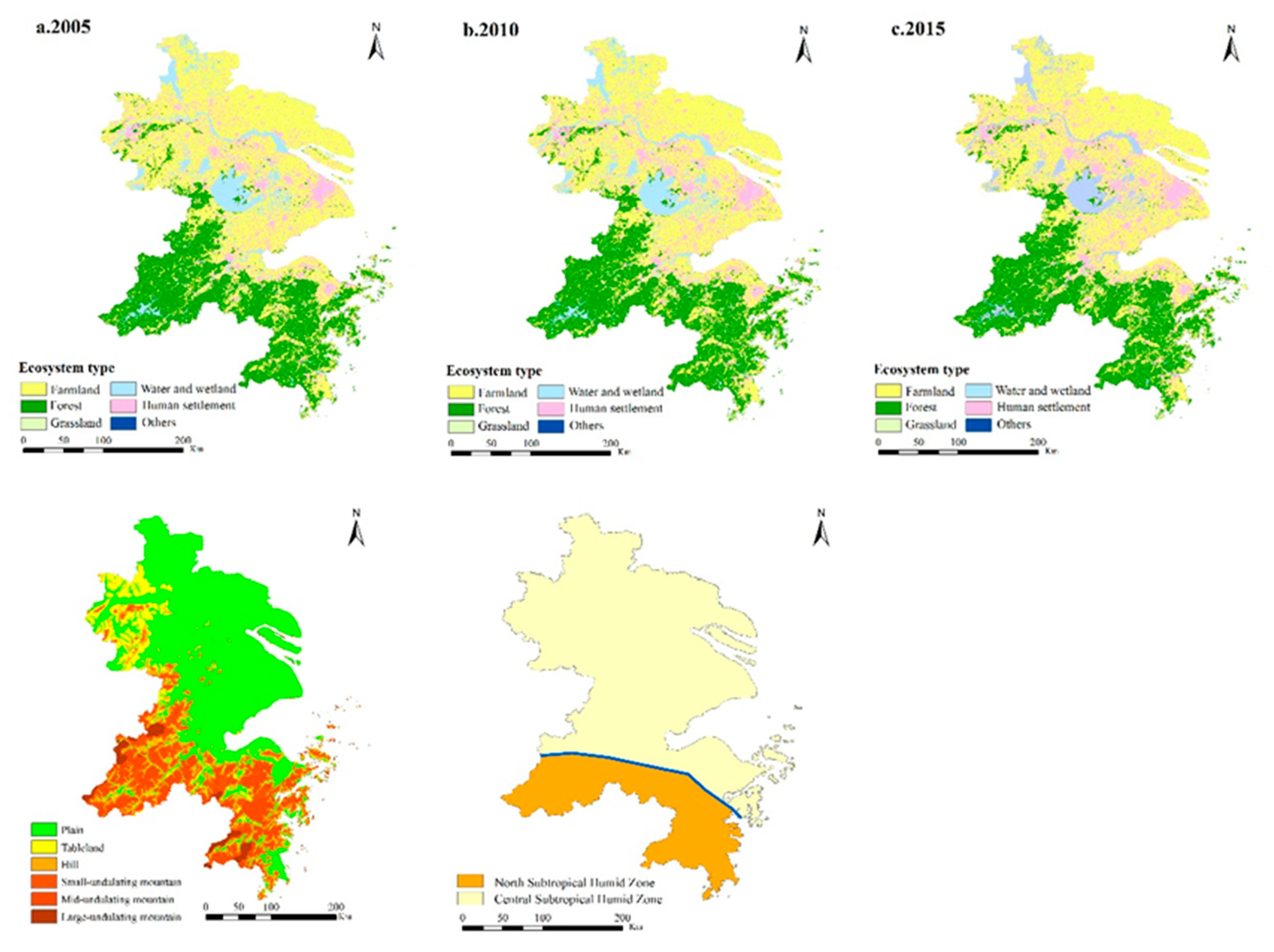
2.2.3. Natural Factors

The Geomor, CR and ET grid-data used in this study were obtained from RESDC [37]. The spatial and time resolution of the ET and Geomor grid-data are 1 km × 1 km for ET and 0.1° × 0.1° for Geomor and one year, respectively.

2.3. Data Preprocessing

All research data were raster data except for the boundary data of the YRD. The raster and vector data differed in structure and form and are therefore difficult to integrate. Thus, we used converting transforming coordinates and applied geometric corrections to standardize the data in ArcGIS 10.3.1. Because the resolution of PD and GDP grid-data and the other data were not the same, we converted the 1 km × 1 km data (PD grid-data, GDP grid-data and ET grid-data) to 0.1° × 0.1° in ArcGIS 10.3.1 to ensure consistent spatial resolution.
We used a subset of the global annual PM2.5 grid-data, Geomor grid-data, ET, CE grid-data, PD grid-data and GDP grid-data in raster format for the YRD from 2005–2015 to produce a 0.1° × 0.1° grid covering the YRD urban cluster using ArcGIS 10.3.1. The 0.1° × 0.1° grid-data was used as the basic spatial unit.

2.4. Methodology

The geographical detector model is a method used to explore differences in graphical elements and their influencing factors on the spatial distributions of a research object [38]. The geographical detector model consists of four parts: factor detectors, interaction detectors, ecological detectors and risk detectors. The factor detectors are mainly used to test whether socioeconomic factors and natural factors are the causes of haze formation. Risk detectors are mainly used to reveal the high and low mean values of the sub-regions of the driving factors. The advantages of the geographical detector model are that it relies on few assumptions and can effectively overcome the limitations of traditional statistical methods for dealing with categorical variables. At present, it is widely used in the ecological and environmental fields [39,40,41].
In our study, we used factor detectors and risk detectors to evaluate socioeconomic factors and natural factors associated with PM2.5 pollution as determined by spatial variance analysis (SVA). The fundamental purpose of SVA is to assess the spatial consistency of PM2.5 concentration distributions versus socioeconomic factors (e.g., PD, GDP, CE) and natural factors (e.g., Geomor, CR, ET).
(1) Factor detector
The power of determinants of driving factors on PM2.5 concentration can be expressed using the following equation:
P D , P = 1 1 n * σ 2 h = 1 L n h * σ h 2
where, P D , P is the power of determinant of a driving factor on PM2.5 concentration.   D is the driving factor for the change in average annual concentration of PM2.5. n ,   σ 2 are sample size and variance of the study area as a whole, respectively.   n h , σ h are sample size and variance of stratum h(h = 1 , 2 ,   L ), respectively. The value of P D , P ranges from 0 to 1. As the value of P D , P approaches 1, the stronger the influence of factor D on changes in average annual concentration of PM2.5.
(2) Risk detector
Risk detectors are mainly used to reveal the high and low mean values of the sub-regions of the driving factors.
t i j = R i R j δ i 2 n i + δ j 2 n j
where, R i , R j represents average PM2.5 concentrations in subregion R ; n represents the size of the sample in subregion R ; and δ represents the variance of subregion R. The geographical detector models used in this study are freely available from (http://www.geodetector.cn/). Since the model requires input data to be type data, the resolution criteria for various data can be found in the Supplementary Materials. The spatial statistical methods used in this paper are mainly raster statistical analysis. Specifically, the statistical analysis was performed using a raster calculator. Because it is simple, it is not described in detail here.

3. Results

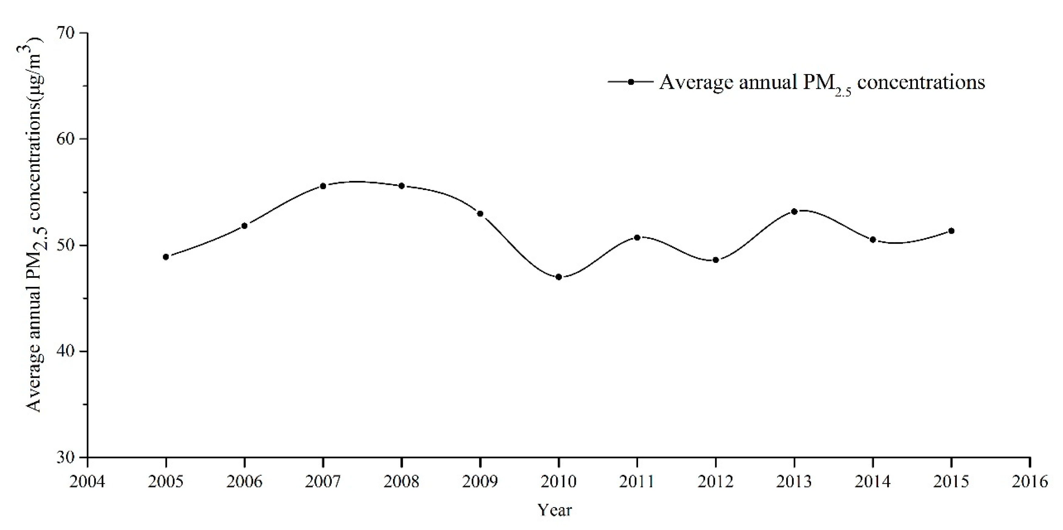
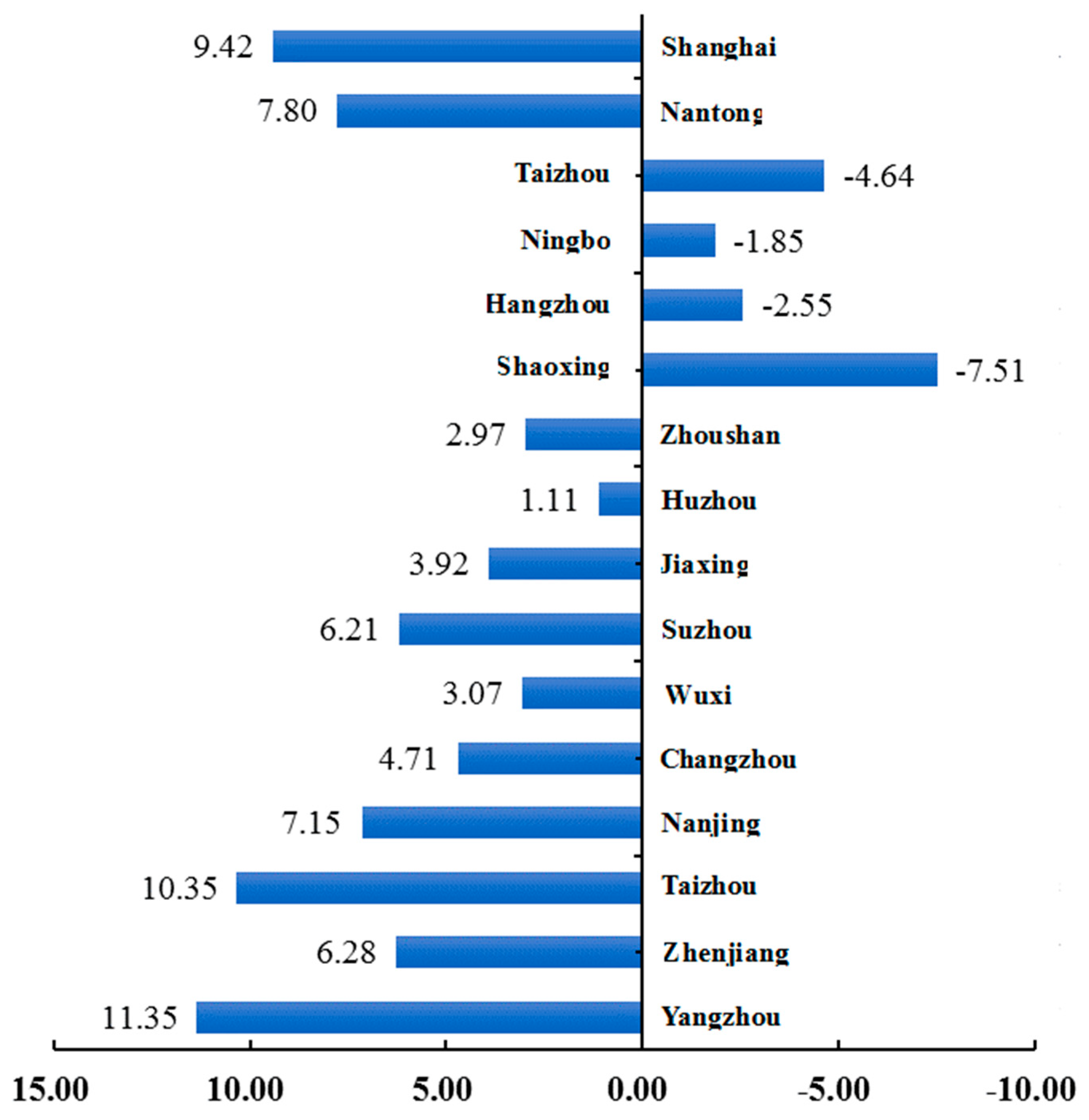
3.1. Spatial Distribution Characteristics of PM2.5 Concentrations

The trend of PM2.5 concentrations in the YRDpresented complex trend from 2005 to 2015 (Figure 3). The raster calculation method for spatial statistical analysis showed that the trend increased from 2005 to 2007, decreased from 2007 to 2010 and fluctuated around 50.22 μg/m3 between 2010 and 2015. The average annual PM2.5 concentration increased from 48.89 μg/m3 in 2005 to 55.56 μg/m3 in 2007, with an average annual increase of 3.33 μg/m3, showing a significant upward trend. This trend became suppressed and turned into a downward trend after 2007. After 2010, average annual PM2.5 concentration fluctuated relatively stable. This indicates that 2007 was an important “inflection point” for the trend in average annual PM2.5 concentration in the YRD, which is consistent with the results released by the Chinese Ministry of Environmental Protection in 2007. The main reasons for the inflection were national ecological civilization construction projects, ecological compensation pilot projects, a pollution census and environmental protection policies. Adjustments to the national industrial structure and improvements in energy efficiency have inhibited particulate emissions to a certain extent.
Using the annual average concentration limit of PM2.5 concentrations in China’s Environmental Air Quality Standards (GB3095-2012), we divided the average annual PM2.5 concentrations into five intervals [42]: level I (<25 μg/m3), level II (25–35 μg/m3), level III (35–50 μg/m3), level IV (50–70 μg/m3) and level V (>70 μg/m3). Further analysis of the area ratio of each interval grid revealed that during the period from 2005 to 2015, the proportion of level I concentrations increased from 1.98% in 2005 to 10.34% in 2015. The proportion of level III concentrations and higher continuously decreased from 78.59% in 2005 to 72.39% in 2015. The proportion of level V concentrations continuously increased from 0.00% in 2005 to 7.75% in 2015, showing a rapid expansion trend in the YRD (Figure 4). The proportion of level I and level V concentration gradually increased from 2005 to 2010. The combined total of level III and level IV concentrations covered about half of the study area. The proportion of the study area that reached the level III and level IV limit was 78.59% in 2005 and 64.64% in 2015 based on the ambient air quality standard (GB3095-2012). The combined total of II concentrations covered about one fifth of the study area. The proportion of the study area that reached the level II limit was 21.41% in 2005 and 27.61% in 2015.
Regions with increasing PM2.5 concentrations were primarily located in the provinces of Jiangsu and Shanghai and included the cities of Yangzhou, Taizhou and Shanghai. The areas with decreasing PM2.5 concentrations were mainly located in Zhejiang Province and included the cities of Hangzhou, Taizhou and Shaoxing (Figure 5). Specifically, average annual PM2.5 concentrations in Yangzhou and Taizhou increased by more than 10 μg/m3 from 2005 to 2015. The average annual PM2.5 concentrations in Shaoxing decreased by more than 5 μg/m3 from 2005 to 2015 (Figure 5).

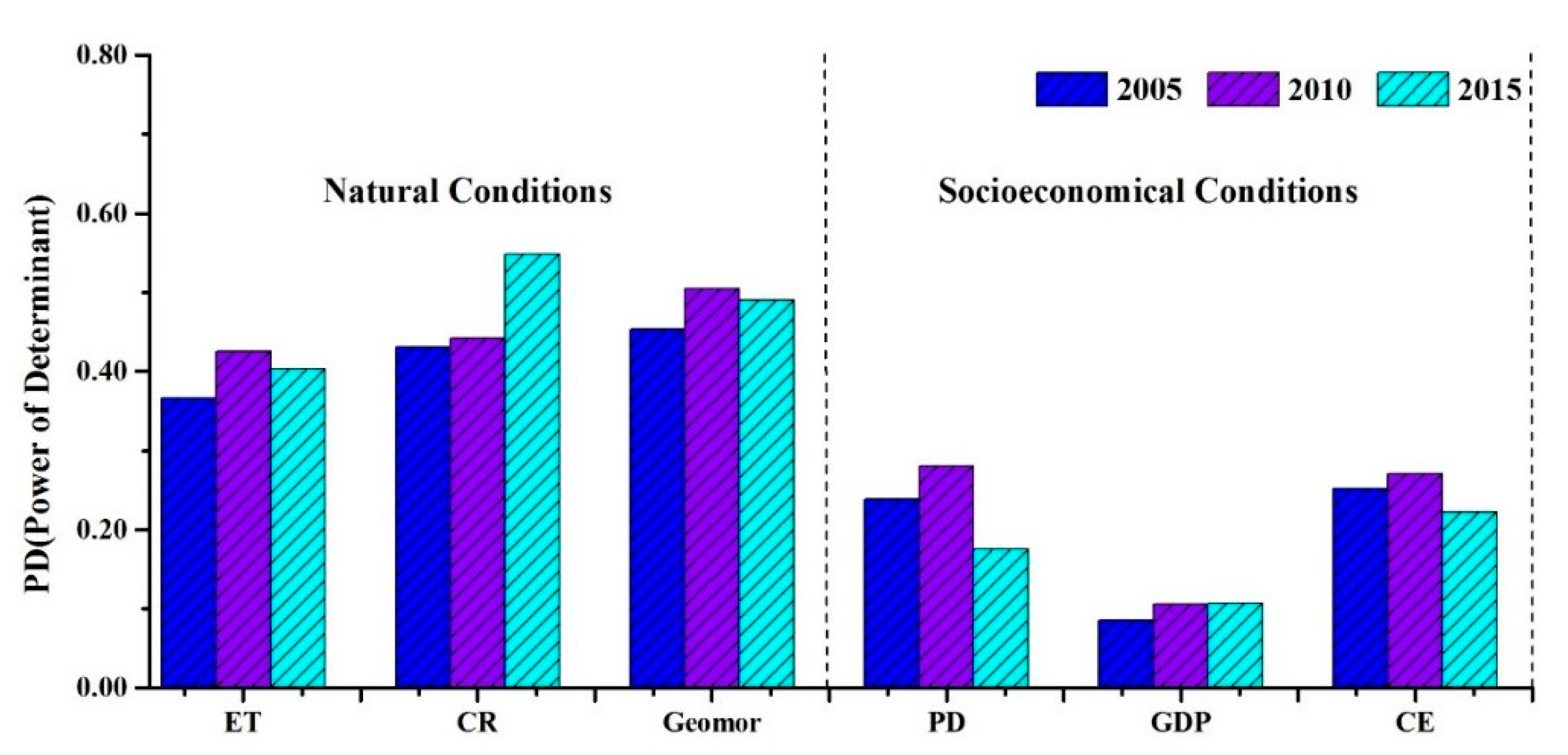
3.2. Individual Effects of Different Factors on PM2.5 Concentrations

The influence of the six natural and socioeconomic risk factors on PM2.5 concentrations were detected using the geographical detector model and are presented in Figure 6. Our results show that Geomor exerted the greatest influence on PM2.5 concentrations, followed by another natural factor, CR. CE was the main socioeconomic factor affecting PM2.5 concentration, followed by PD. The natural conditions exerted a greater influence over PM2.5 concentrations in the YRD than did socioeconomic conditions in 2005, 2010 and 2105. Specifically, Geomor(0.45) > CR(0.43) > ET(0.36) > CE(0.25) > PD(0.23) > GDP(0.085) in 2005; Geomor(0.50) > CR(0.44) > ET(0.42) > PD(0.28) > CE(0.27) > GDP(0.10) in 2010; CR(0.54) > Geomor(0.49) > ET(0.40) > CE(0.22) > PD(0.17) > GDP(0.10) in 2015.

3.3. The Leading Impact Areas of Factors Influencing PM2.5 Concentrations

For the years 2005, 2010 and 2015, average PM2.5 concentrations were highest in the subregion of the human settlement ecosystem (54.87 μg/m3, 53.97 μg/m3 and 59.98 μg/m3), followed by the farmland ecosystem (54.62 μg/m3, 53.27 μg/m3 and 58.77 μg/m3) and the wetland ecosystem (54.58 μg/m3, 51.77 μg/m3 and 57.96 μg/m3). Average PM2.5 concentrations were highest in the north subtropic humid climate subregion (52.92 μg/m3, 51.27 μg/m3 and 57.52 μg/m3) and the central subtropic humid climate subregion (35.11 μg/m3, 31.89 μg/m3 and 29.23 μg/m3). And finally, average PM2.5 concentrations were highest in the geomorphological plain subregion (54.43 μg/m3, 54.49 μg/m3 and 60.71 μg/m3), followed by the platform subregion (53.97 μg/m3, 51.6 μg/m3 and 56.21 μg/m3) and the hilly subregion (Figure 7).

4. Discussion

A better understanding of the factors influencing the spatial distribution of PM2.5 concentrations benefits managers tasked with formulating air pollution control strategies. Using spatial statistical analysis and a geographical detector model, this study emphasizes the importance of socioeconomic and natural factors in determining PM2.5 concentrations. Socioeconomic development is a main cause of PM2.5 formation and Geomor, CR and ET factors significantly affected its distribution, aggregation and diffusion. We next discuss the impacts of socioeconomic and natural factors on PM2.5 concentrations.

4.1. Analysis of The Socioeconomic Drivers of PM2.5 Pollution

Socioeconomic activities profoundly impact air pollution and regional emissions of polluting gases are closely related to socioeconomic activities. GDP, CE and PD data represent the level of industrialization and urbanization in the YRD and are important drivers of PM2.5 concentrations. Our factor detector results show that CE and PD were the main influencing factors in all three years of the study and their influence was significantly greater than that of GDP. The relationship between CE and PD exhibited an inverted U-shaped with the inflection point occurring in 2010.
Many studies have shown that socioeconomic factors are the most significant factors influencing PM2.5 concentrations [19,43], with the power of the determinant greater than 50% [44]. Our findings are consistent with these studies. Energy consumption, as represented by CE, was the most important factor triggering PM2.5 formation. The reason that energy consumption exerts the strongest influence is that total energy consumption has significantly increased from 2005 to 2015. Coal is the largest source of energy production in the YRD. For example, total coal consumption in Jiangsu Province has increased by more than 58% from 2005 to 2015. China’s steel industry, which consumed huge amounts of coal from 2005–2015, is mainly located in the YRD, with Jiangsu and Shanghai serving as primary centers of the steel industry. The high level of steel production in Jiangsu Province and Shanghai accounted for an overall increase in national steel production from 17.71% in 2005 to 19.08% in 2015. The spatial agglomeration of the coal and steel industries is a key factor driving increases in PM2.5 concentrations. The curve showing the effects of socioeconomic factors (CE and PD) on PM2.5 contains an inflection point between 2005 and 2015. The reason for the formation of the inflection point may be that the government vigorously controls sulfur dioxide, so that measures such as desulfurization of coal-fired power plants and replacement of coal-fired boilers with clean energy technologies reduces smog. Therefore, China has further opportunities to reduce smog by altering its industrial and energy structures, reducing coal emissions, developing new energy sources and encouraging residents to use mass transportation [45].
In addition to CE, many studies have found that PD affects PM2.5, which is also consistent with our findings. PD may affect PM2.5 through population agglomeration, which leads to increased industrial agglomeration and production activities (e.g., catering industry, service industry, construction industry) and increased pollutant emissions and energy consumption [9]. For example, traffic jams that result from dense population agglomeration reduce the combustion efficiency of motor fuels. In addition, densely packed housing reduces wind speeds and dispersal of pollutants, thereby trapping high PM2.5 concentrations and indirectly aggravating PM2.5 pollution. The reason for the formation of the inflection point may be that increasing PD will also have an agglomeration effect, which will increase the rate of public transportation and the efficiency of resource use, leading to alleviation of PM2.5 pollution. The results of this study suggest that the counter scale effect of population agglomeration played a significant role in PM2.5 pollution before 2010, while the scale effect of population agglomeration played a greater role in PM2.5 pollution after 2010.

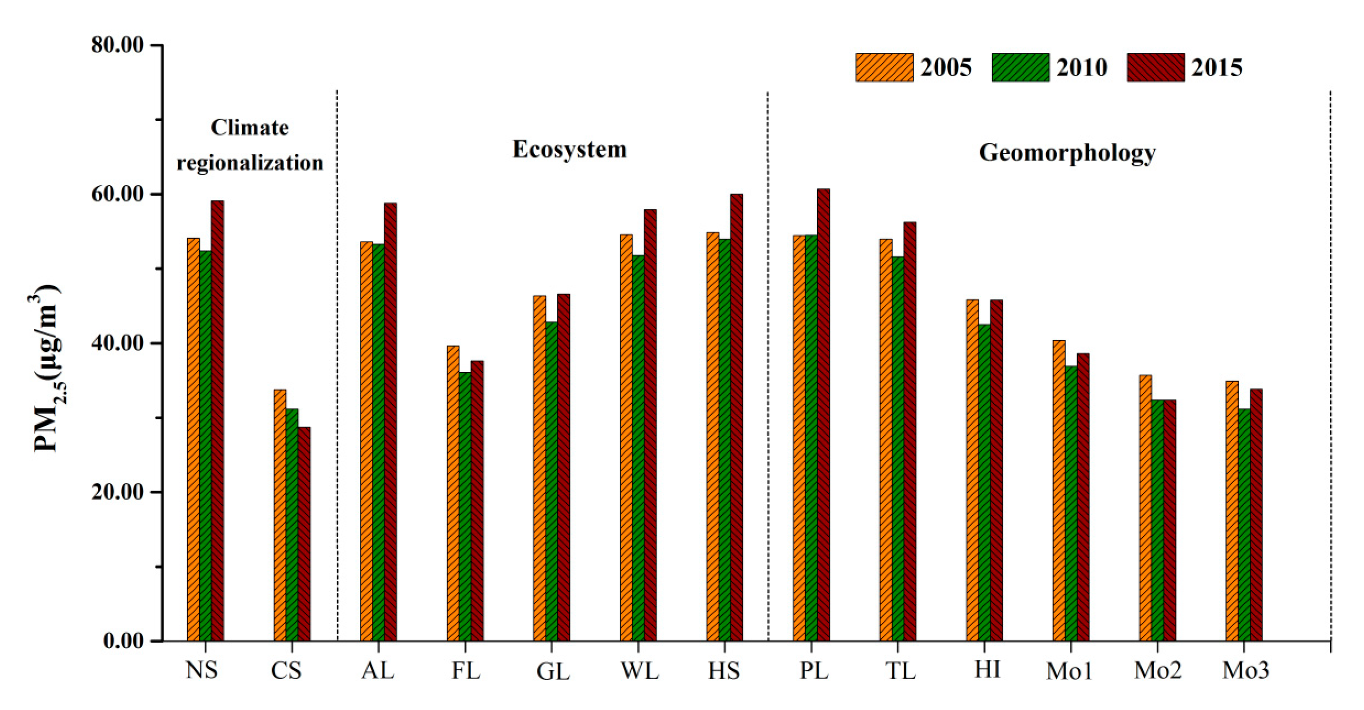
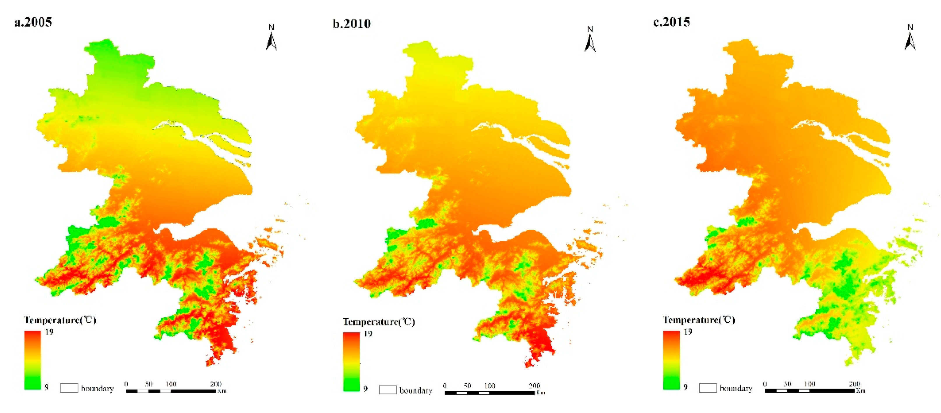
4.2. Analysis of The Natural Drivers of PM2.5 Pollution

Our factor detection results show that Geomor and CR are the main factors affecting PM2.5 diffusion and that their explanatory power is greater than that of ET. This result demonstrates large-scale spatial heterogeneity and indicates that geomorphology and climate regionalization have an important influence on the agglomeration and diffusion of PM2.5 [20]. Our findings are consistent with many studies [46,47]. Geomor and CR likely affect PM2.5 agglomeration and diffusion by affecting air flow, air pressure, temperature and precipitation [26,46]. There are several possible explanations for this finding. As a fine particle, PM2.5 floats easily in low altitudes compared with high altitudes due to gravity. On the other hand, as altitude increases, temperature gradually decrease and air convection increases, resulting in increased mobility of PM2.5 particles. Therefore, PM2.5 concentrations in low altitudes areas are higher than in high altitude areas [48].
The effect of CR on PM2.5 concentrations is mainly via temperature and precipitation. This may be related to the uneven rainfall and temperature differences in the YRD. There are significant differences in precipitation and temperature between the north and the south (Figure 8 and Figure 9). The YRD is spread over two climatic zones. The northern part is a north subtropical humid zone, while the south is a central subtropical humid zone. There are several possible explanations for the impact of temperature and precipitation on PM2.5 concentrations: (1) Raindrops (or other precipitation particles) capture aerosol particles from the atmosphere during Brownian diffusion, inertial collision and other processes, resulting in a decrease in PM2.5 concentration [49,50,51,52]. This may explain the decline in PM2.5 concentration in 2010 (Table 2); (2) The primary mode of diffusion of suspended particulates in the air is Brownian motion. The intensity of Brownian motion is related to temperature. Therefore, the higher the atmospheric temperature, the more intense the Brownian motion of the fine particles and the more favorable the diffusion of the particles [53,54]. The results of this study are limited to the YRD region from 2005 to 2015. Although the impact of ET was lower than the other two impact factors, we cannot assume that it is not important, especially in the northern plains where fertilizers used in farmland ecosystems strongly affect PM2.5 [55].

4.3. Limitations of This Study

The first limitation of this study is the PM2.5 grid-data. Although the resulting PM2.5 estimates were highly consistent, there is some uncertainty resulting from the sparse dispersal of PM2.5 monitoring sites and the challenging nature of data retrieval and validation [31]. The second limitation comes from the socioeconomic data. In this study, the socioeconomic factors included only GDP, PD and CE, which cannot comprehensively express the characteristics of socioeconomic factors. The third limitation is that the GDP and population density products used in this study were derived from national economic census and national population census data. Because the survey periods for these censuses are long, the time resolution for the data is rough. In order to balance the spatial resolution and temporal resolution of the various socioeconomic and natural ecological factors, five years was chosen as the research cycle. In addition, we only focused on the spatial variation characteristics and driving factors of PM2.5 at three time points, which limits the scope of this study. In future research, we will focus on longer time series of annual PM2.5 data to more accurately delineate the spatial variation characteristics of PM2.5 and quantitatively reveal the influences of socioeconomic and natural factors on PM2.5 concentrations in the YRD.

5. Conclusions

Based on remote sensing inversion of PM2.5 concentration data over a long time series, our spatial statistical analyses and geographical detector model revealed the spatial distribution and variation characteristics of PM2.5 and the main influencing factors of PM2.5 concentrations in the YRD from 2005 to 2015. Our main findings and conclusions are as follows:
(1) Average annual PM2.5 concentrations in the YRD displayed an increasing trend prior to 2007, a downward trend after 2007 and then eventually stabilized. The proportion of highly polluted areas (PM2.5 greater than 70 μg/m3) gradually increased between 2005 and 2015 andwere mainly located in the northern regions of the YRD, especially Yangzhou, Taizhou and Zhenjiang. The proportion of low-pollution areas (PM2.5 less than 35 μg/m3) gradually decreased and were mainly located in southern YRD, especially Shaoxing, Taizhou and Ningbo. (2) The natural driving factors CR and Geomor were the dominant individual factors affecting PM2.5 concentration diffusion, while CE and PD were the dominant individual factors affecting PM2.5 formation. Natural factors and socio-economic factors together lead to increased PM2.5 pollution. Natural factors and socioeconomic factors together lead to PM2.5 pollution. Although our research data are from the YRD, our research method and framework can be applied in pollution prevention and control efforts in other regions. These findings extend our understanding of potential socioeconomic and natural drivers of PM2.5 concentrations and can help policy makers in their tasks of formulating pollution control strategies and improving air quality.

Supplementary Materials

The following are available online at https://www.mdpi.com/2073-4433/10/2/55/s1.

Author Contributions

G.Y. conceived and performed the experiments and wrote the first draft. Y.H., Y.J., P.D. and S.D. did portion of the data processing and translation. All authors contributed to and approved the final manuscript.

Funding

This work was supported by the Open Fund of the Big Data Institute of Digital Natural Disaster Monitoring in Fujian (NDMBD2018001) and the Natural Science Foundation of Fujian Province (2016J01199). We would like to thank Chengdong Xu and Zhifeng Wu for their helpful suggestions.

Conflicts of Interest

The authors declare no conflict of interest. Guoliang Yun and Yuanrong He contributed equally to this work and should be considered co- correspondence authors.

References

  1. Dockery, D.W.; Pope, C.A.; Xu, X.; Spengler, J.D.; Ware, J.H.; Fay, M.E.; Ferris, B.G.; Speizer, F.E. An Association between Air Pollution and Mortality in Six U.S. Cities. N. Engl. J. Med. 1993, 329, 1753–1759. [Google Scholar] [CrossRef]
  2. Meredith, F.; Petros, K.; Petros, S. The role of particle composition on the association between PM2.5 and mortality. Epidemiology 2008, 19, 680–689. [Google Scholar]
  3. Ardenpopeiii, C. Review: Epidemiological Basis for Particulate Air Pollution Health Standards. Aerosol Sci. Technol. 2000, 32, 4–14. [Google Scholar] [Green Version]
  4. Yun, G.L.; Zuo, S.D.; Dai, S.Q.; Song, X.D.; Xu, C.D.; Liao, Y.L.; Zhao, P.Q.; Chang, W.Y.; Chen, Q.; Li, Y.Y.; et al. Individual and Interactive Influences of Anthropogenic and Ecological Factors on Forest PM2.5 Concentrations at an Urban Scale. Remote Sens. 2018, 10, 521. [Google Scholar] [CrossRef]
  5. Lelieveld, J.; Evans, J.S.; Fnais, M.; Giannadaki, D.; Pozzer, A. The contribution of outdoor air pollution sources to premature mortality on a global scale. Nature 2015, 525, 367–371. [Google Scholar] [CrossRef]
  6. Lim, S.S.; Vos, T.; Flaxman, A.D.; Danaei, G.; Shibuya, K.; Adair-Rohani, H.; AlMazroa, M.A.; Amann, M.; Anderson, H.R.; Andrews, K.G. A comparative risk assessment of burden of disease and injury attributable to 67 risk factors and risk factor clusters in 21 regions, 1990–2010: A systematic analysis for the Global Burden of Disease Study 2010. Lancet 2012, 380, 2224–2260. [Google Scholar] [CrossRef]
  7. Group, G.M.W. Burden of Disease Attributable to Coal-Burning and Other Major Sources of Air Pollution in China; Health Effects Institute: Boston, MA, USA, 2016. [Google Scholar]
  8. Fu, Q.Y.; Zhuang, G.S.; Wang, J.; Xu, C.; Huang, K.; Li, J.; Hou, B.; Lu, T.; Streets, D.G. Mechanism of formation of the heaviest pollution episode ever recorded in the Yangtze River Delta, China. Atmos. Environ. 2008, 42, 2023–2036. [Google Scholar] [CrossRef]
  9. Lou, C.R.; Liu, H.Y.; Li, Y.F.; Li, Y.L. Socioeconomic Drivers of PM2.5 in the Accumulation Phase of Air Pollution Episodes in the Yangtze River Delta of China. Int. J. Environ. Res. Public Health 2016, 13, 928. [Google Scholar] [CrossRef]
  10. Liu, Y.; Park, R.J.; Jacob, D.J.; Li, Q.; Kilaru, V.; Sarnat, J.A. Mapping annual mean ground-level PM2.5 concentrations using Multiangle Imaging Spectroradiometer aerosol optical thickness over the contiguous United States. J. Geophys. Res. Atmos. 2004, 109. [Google Scholar] [CrossRef]
  11. Liu, Y. Monitoring PM2.5 from space for health: Past, present and future directions. EM (Pittsburgh Pa) 2014, 6, 6–10. [Google Scholar]
  12. Chudnovsky, A.A.; Lee, H.J.; Kostinski, A.; Kotlov, T.; Koutrakis, P. Prediction of daily fine particulate matter concentrations using aerosol optical depth retrievals from the Geostationary Operational Environmental Satellite (GOES). J. Air Waste Manag. Assoc. 2012, 62, 1022–1031. [Google Scholar] [CrossRef] [Green Version]
  13. Nguyen, T.; Yu, X.; Zhang, Z.; Liu, M.; Liu, X. Relationship between types of urban forest and PM2.5 capture at three growth stages of leaves. J. Environ. Sci. 2015, 27, 33–41. [Google Scholar] [CrossRef]
  14. Lu, D.; Xu, J.; Yang, D.; Zhao, J. Spatio-temporal variation and influence factors of PM2.5 concentrations in China from 1998 to 2014. Atmos. Pollut. Res. 2017, 8, 1151–1159. [Google Scholar] [CrossRef]
  15. Paatero, P.; Hopke, P.K.; Hoppenstock, J.; Eberly, S.I. Advanced factor analysis of spatial distributions of PM2.5 in the eastern United States. Environ. Sci. Technol. 2003, 37, 2460–2476. [Google Scholar] [CrossRef]
  16. Wang, S.; Fang, C.; Wang, Y.; Huang, Y.; Ma, H. Quantifying the relationship between urban development intensity and carbon dioxide emissions using a panel data analysis. Ecol. Indic. 2015, 49, 121–131. [Google Scholar] [CrossRef]
  17. Guo, S.; Hu, M.; Zamora, M.L.; Peng, J.; Shang, D.; Zheng, J.; Du, Z.; Wu, Z.; Shao, M.; Zeng, L.; et al. Elucidating severe urban haze formation in China. Proc. Natl. Acad. Sci. USA 2014, 111, 17373–17378. [Google Scholar] [CrossRef] [Green Version]
  18. Zhou, L.; Zhou, C.; Yang, F.; Wang, B.; Sun, D. Spatio-temporal evolution and the influencing factors of PM2.5 in China between 2000 and 2011. Acta Geogr. Sin. 2017, 29, 253–270. [Google Scholar] [CrossRef]
  19. Yang, D.; Wang, X.; Xu, J.; Xu, C.; Lu, D.; Ye, C.; Wang, Z.; Bai, L. Quantifying the influence of natural and socioeconomic factors and their interactive impact on PM2.5 pollution in China. Environ. Pollut. 2018, 241, 475–483. [Google Scholar] [CrossRef]
  20. Liu, H.; Fang, C.; Zhang, X.; Wang, Z.; Bao, C.; Li, F. The effect of natural and anthropogenic factors on haze pollution in Chinese cities: A spatial econometrics approach. J. Clean Prod. 2017, 165, 323–333. [Google Scholar] [CrossRef]
  21. Artíñano, B.; Salvador, P.; Alonso, D.G.; Querol, X.; Alastuey, A. Anthropogenic and natural influence on the PM10 and PM2.5 aerosol in Madrid (Spain). Analysis of high concentration episodes. Environ. Pollut. 2003, 125, 453–465. [Google Scholar] [CrossRef]
  22. Bechle, M.J.; Millet, D.B.; Marshall, J.D. Effects of Income and Urban Form on Urban NO2: Global Evidence from Satellites. Environ. Sci. Technol. 2011, 45, 4914–4919. [Google Scholar] [CrossRef]
  23. Wu, J.S.; Wang, X.; Li, J.C.; Tu, Y.J. Comparison of Models on Spatial Variation of PM2.5 Concentration: A Case of Beijing-Tianjin-Hebei Region. Environ. Sci. 2017, 38, 2191–2201. [Google Scholar]
  24. Akimoto, H. Global Air Quality and Pollution. Science 2003, 302, 1716–1719. [Google Scholar] [CrossRef] [Green Version]
  25. Li, G.; Fang, C.; Wang, S.; Sun, S. The Effect of Economic Growth, Urbanization, and Industrialization on Fine Particulate Matter (PM2.5) Concentrations in China. Environ. Sci. Technol. 2016, 50, 11452–11459. [Google Scholar] [CrossRef] [PubMed]
  26. Bravo Alvarez, H.; Sosa Echeverria, R.; Sanchez Alvarez, P.; Krupa, S. Air Quality Standards for Particulate Matter (PM) at high altitude cities. Environ. Pollut. 2013, 173, 255–256. [Google Scholar] [CrossRef] [PubMed]
  27. Cao, C.; Lee, X.; Liu, S.; Schultz, N.; Xiao, W.; Zhang, M.; Zhao, L. Urban heat islands in China enhanced by haze pollution. Nat. Commun. 2016, 7, 12509. [Google Scholar] [CrossRef] [Green Version]
  28. Wang, S.; Li, G.; Fang, C. Urbanization, economic growth, energy consumption, and CO2 emissions: Empirical evidence from countries with different income levels. Renew. Sustain. Energy Rev. 2018, 81, 2144–2159. [Google Scholar] [CrossRef]
  29. Wang, S.; Zhou, C.; Li, G.; Feng, K. CO2, economic growth, and energy consumption in China’s provinces: investigating the spatiotemporal and econometric characteristics of China’s CO2 emissions. Ecol. Indic. 2016, 69, 184–195. [Google Scholar] [CrossRef]
  30. Atmospheric Composition Analysis Group. Available online: http://fizz.phys.dal.ca/~atmos/martin/?page_id 140 (accessed on 18 August 2018).
  31. Van, D.A.; Martin, R.V.; Brauer, M.; Hsu, N.C.; Kahn, R.A.; Levy, R.C.; Lyapustin, A.; Sayer, A.M.; Winker, D.M. Global Estimates of Fine Particulate Matter using a Combined Geophysical-Statistical Method with Information from Satellites, Models, and Monitors. Environ. Sci. Technol. 2016, 50, 3762–3772. [Google Scholar]
  32. Seung-Jae, L.; Serre, M.L.; Aaron, V.D.; Martin, R.V.; Burnett, R.T.; Michael, J. Comparison of Geostatistical Interpolation and Remote Sensing Techniques for Estimating Long-Term Exposure to Ambient PM2.5 Concentrations across the Continental United States. Environ. Health Perspect. 2012, 120, 1727–1732. [Google Scholar]
  33. de Sherbinin, A.; Levy, M.A.; Zell, E.; Weber, S.; Jaiteh, M. Using satellite data to develop environmental indicators. Environ. Res. Lett. 2014, 9, 084013. [Google Scholar] [CrossRef] [Green Version]
  34. Luo, J.; Du, P.; Samat, A.; Xia, J.; Che, M.; Xue, Z. Spatiotemporal Pattern of PM2.5 Concentrations in Mainland China and Analysis of Its Influencing Factors using Geographically Weighted Regression. Sci. Rep. 2017, 7, 40607. [Google Scholar] [CrossRef]
  35. Chen, H.; Huang, Y.; Shen, H.; Chen, Y.; Ru, M.; Chen, Y.; Lin, N.; Su, S.; Zhuo, S.; Zhong, Q.; et al. Modeling temporal variations in global residential energy consumption and pollutant emissions. Appl. Energy 2016, 184, 820–829. [Google Scholar] [CrossRef]
  36. China Emission Accounts and Datasets. Available online: http://inventory.pku.edu.cn/download/download.html (accessed on 18 August 2018).
  37. RESDC (Data Center for Resources and Environmental Sciences, Chinese Academy of Sciences). Available online: http://www.resdc.cn (accessed on 18 August 2018).
  38. Wang, J.F.; Li, X.H.; Christakos, G.; Liao, Y.L.; Zhang, T.; Gu, X.; Zheng, X.Y. Geographical detectors-based health risk assessment and its application in the neural tube defects study of the Heshun Region, China. Int. J. Geogr. Inf. Sci. 2010, 24, 107–127. [Google Scholar] [CrossRef]
  39. Qiao, P.; Lei, M.; Guo, G.; Yang, J.; Zhou, X.; Chen, T. Quantitative Analysis of the Factors Influencing Soil Heavy Metal Lateral Migration in Rainfalls Based on Geographical Detector Software: A Case Study in Huanjiang County, China. Sustainability 2017, 9, 1227. [Google Scholar] [CrossRef]
  40. Zhang, N.; Jing, Y.-C.; Liu, C.-Y.; Li, Y.; Shen, J. A cellular automaton model for grasshopper population dynamics in Inner Mongolia steppe habitats. Ecol. Model. 2016, 329, 5–17. [Google Scholar] [CrossRef]
  41. Shen, J.; Zhang, N.; He, B.; Liu, C.Y.; Li, Y.; Zhang, H.Y.; Chen, X.Y.; Lin, H. Construction of a GeogDetector-based model system to indicate the potential occurrence of grasshoppers in Inner Mongolia steppe habitats. Bull. Entomol. Res. 2015, 105, 335–346. [Google Scholar] [CrossRef]
  42. Samet, J.M.; Dominici, F.; Curriero, F.C.; Coursac, I.; Zeger, S.L. Fine particulate air pollution and mortality in 20 US cities, 1987–1994. N. Engl. J. Med. 2000, 343, 1742–1749. [Google Scholar] [CrossRef]
  43. Zhou, C.; Chen, J.; Wang, S. Examining the effects of socioeconomic development on fine particulate matter (PM2.5) in China’s cities using spatial regression and the geographical detector technique. Sci. Total Environ. 2018, 619–620, 436–445. [Google Scholar] [CrossRef]
  44. Jiang, P.; Yang, J.; Huang, C.; Liu, H. The contribution of socioeconomic factors to PM2.5 pollution in urban China. Environ. Pollut. 2018, 233, 977–985. [Google Scholar] [CrossRef]
  45. Redman, L.; Friman, M.; Gärling, T.; Hartig, T. Quality attributes of public transport that attract car users: A research review. Transp. Policy 2013, 25, 119–127. [Google Scholar] [CrossRef]
  46. Cisneros, R.; Schweizer, D.; Preisler, H.; Bennett, D.H.; Shaw, G.; Bytnerowicz, A. Spatial and seasonal patterns of particulate matter less than 2.5 microns in the Sierra Nevada Mountains, California. Atmos. Pollut. Res. 2014, 5, 581–590. [Google Scholar] [CrossRef] [Green Version]
  47. Zhang, T.H.; Liu, G.; Zhu, Z.M.; Gong, W.; Ji, Y.X.; Huang, Y.S. Real-Time Estimation of Satellite-Derived PM2.5 Based on a Semi-Physical Geographically Weighted Regression Model. Int. J. Environ. Res. Public Health 2016, 13, 974. [Google Scholar] [CrossRef] [PubMed]
  48. Halsey, L.A.; Vitt, D.H.; Zoltai, S.C. Disequilibrium response of permafrost in boreal continental western Canada to climate change. Clim. Chang. 1995, 30, 57–73. [Google Scholar] [CrossRef]
  49. Çuhadaroğlu, B.; Demirci, E. Influence of Some Meteorological Factors on Air Pollution in Trabzon City. Energy Build. 1997, 25, 179–184. [Google Scholar] [CrossRef]
  50. Li, L.; Qian, J.; Ou, C.Q.; Zhou, Y.X.; Guo, C.; Guo, Y. Spatial and temporal analysis of Air Pollution Index and its timescale-dependent relationship with meteorological factors in Guangzhou, China, 2001–2011. Environ. Pollut. 2014, 190, 75–81. [Google Scholar] [CrossRef] [PubMed]
  51. Tai, A.P.K.; Mickley, L.J.; Jacob, D.J. Correlations between fine particulate matter (PM2.5) and meteorological variables in the United States: Implications for the sensitivity of PM2.5 to climate change. Atmos. Environ. 2010, 44, 3976–3984. [Google Scholar] [CrossRef]
  52. Jianming, X.U.; Gao, W.; Yuanhao, Q.U. Observation of the wet scavenge effect of rainfall on PM2.5 in Shanghai. Acta Sci. Circumst. 2017, 37, 3271–3279. [Google Scholar]
  53. Megaritis, A.; Fountoukis, C.; Charalampidis, P.; Denier Van Der Gon, H.; Pilinis, C.; Pandis, S. Linking climate and air quality over Europe: Effects of meteorology on PM2.5 concentrations. Atmos. Chem. Phys. 2014, 14, 10283–10298. [Google Scholar] [CrossRef]
  54. Liu, X.-H.; Yu, X.-X.; Zhang, Z.-M.; Liu, M.-M.; Ruanshi, Q.-C. Pollution characteristics of atmospheric particulates in forest belts and their relationship with meteorological conditions. J. Ecol. 2014, 33, 1715–1721. [Google Scholar]
  55. Wang, G.; Zhang, R.; Gomez, M.E.; Yang, L.; Zamora, M.L.; Hu, M.; Lin, Y.; Peng, J.; Guo, S.; Meng, J. Persistent sulfate formation from London Fog to Chinese haze. Proc. Natl. Acad. Sci. USA 2016, 113, 13630–13635. [Google Scholar] [CrossRef] [PubMed] [Green Version]
  56. Xu, J.H.; Jiang, H. Estimation of PM2.5 Concentration over the Yangtze Delta Using Remote Sensing: Analysis of Spatial and Temporal Variations. Huan jing ke xue=Huanjing kexue 2015, 36, 3119–3127. [Google Scholar] [PubMed]
Figure 1. The spatial distribution of socioeconomic factors.
Atmosphere 10 00055 g001
Figure 2. The spatial distribution of natural factors.
Atmosphere 10 00055 g002
Figure 3. Overall trend for PM2.5 concentrations in the Yangtze River Delta (YRD) from 2005–2015.
Atmosphere 10 00055 g003
Figure 4. The spatial distribution of changes in annual average PM2.5 concentrations in different YRD cities from 2005 to 2015.
Atmosphere 10 00055 g004
Figure 5. Average annual changes in PM2.5 concentrations (μg/m3) in different YRD cities from 2005 to 2015.
Atmosphere 10 00055 g005
Figure 6. The power of determinants of different impact factors (ET, CR, Geomor, PD, GDP and CE) on PM2.5 concentrations in the YRD (p-values < 0.01 for all factors).
Atmosphere 10 00055 g006
Figure 7. Annual average PM2.5 concentrations in different climate, ecosystem and geomorphological subregions (NS = North subtropical humid zone, CS = Central subtropical humid zone, AL = Arable land ecosystem, FL=Forest ecosystem, GL = Grassland ecosystem, WL = Water and wetland ecosystem, HS = Human settlement ecosystem, PL = Plain, TL = Tableland, HI = Hills, Mo1 = Small-undulating mountain, Mo2 = Mid-undulating mountain, Mo3 = Large-undulating mountain).
Atmosphere 10 00055 g007
Figure 8. Spatial distribution of average annual precipitation in (a) 2005, (b) 2010, (c) 2015 in the YRD.
Atmosphere 10 00055 g008
Figure 9. Spatial distribution of average annual temperature in (a) 2005, (b) 2010, (c) 2015 in the YRD.
Atmosphere 10 00055 g009
Table 1. Socioeconomic and natural factors analyzed as potential driving factors of the spatial variation of PM2.5 concentration.
Explanatory VariableNameSymbolUnitBrief Description
Socioeconomic FactorsPopulation densityPD peoples / km 2 Population scale
Gross Domestic ProductGDPyuan/ km 2 Level of economic development
Total CO2 emissionsCEtonEnergy consumption
Natural FactorsGeomorphologyGeomor-Topographical features
Climate regionalizationCR-Precipitation and temperature
Ecosystem typeET-Ecosystem functions
Table 2. Average annual precipitation from 2005 to 2015 (mm·a−1).
YearPrecipitation
MaxMinMeanStandard Deviation
200522205281104321
200617128341188244
200714125841058180
200816137711138107
200917026321286179
201026487181416360
20111712294831244
201223395351369490
201326463961156307
201421638501422254
201523899641643240
Note: The precipitation for 2005–2013 comes from Xu [56] and the precipitation for 2014–2015 was obtained from the Data Center for Resources and Environmental Sciences, Chinese Academy of Sciences (RESDC) (http://www.resdc.cn).

