An Observational Study on Cloud Spectral Width in North China

Abstract

Cloud droplet size distribution (CDSD) is a critical characteristic for a number of processes related to clouds, considering that cloud droplets are formed in different sizes above the cloud-base. This paper analyzes the in-situ aircraft measurements of CDSDs and aerosol concentration ($N_a$) performed in stratiform clouds in Hebei, China, in 2015 to reveal the characteristics of cloud spectral width, commonly known as relative dispersion ($\epsilon$, ratio of standard deviation (σ) to mean radius (r) of the CDSD). A new algorithm is developed to calculate the contributions of droplets of different sizes to $\epsilon$. It is found that small droplets with the size range of 1 to 5.5 μm and medium droplets with the size range of 5.5 to 10 μm are the major contributors to ε, and the medium droplets generally dominate the change of ε. The variation of $\epsilon$ with $N_a$ can be well explained by comparing the normalized changes of $\sigma$ and $r$ ($k_{\sigma }/\sigma$ and $k_r/r$), rather than $k_{\sigma }$ and $k_r$ only ($k_{\sigma }$ is Δσ/Δ$N_a$ and $k_r$ is Δr/Δ$N_a$). From the perspective of external factors affecting $\epsilon$ change, the effects of $N_a$ and condensation are examined. It is found that $\epsilon$ increases initially and decreases afterward as $N_a$ increases, and “condensational broadening” occurs up to 1 km above cloud-base, potentially providing observational evidence for recent numerical simulations in the literature.

1. Introduction

Numerous studies have shown that increasing anthropogenic aerosols have significant effects (direct, semi-direct, and indirect) on weather and climate [1,2,3,4]. It is well known that increasing aerosols tend to increase concentrations of cloud condensation nuclei (CCN) and ice nuclei, and thereby increase concentrations of cloud droplets ($N_c$) and ice crystals. The resultant impact on the optical characteristics and lifecycles of clouds is seen as an indirect effect of aerosols [5]. For a given liquid water content (LWC), an increased aerosol concentration ($N_a$) reduces the effective radius ($r_e$) and enhances the cloud albedo [6,7], a phenomenon known as the Twomey effect. Besides $N_a$ [8], $r_e$ is also related to relative dispersion (ε), the ratio of standard deviation (σ) to mean radius (r) of cloud droplet size distribution (CDSD),

$$r_e=\frac{{\left(1+2{\epsilon }^2\right)}^{2/3}}{{\left(1+{\epsilon }^2\right)}^{1/3}}{\left(\frac{3LWC}{4\pi \rho N_c}\right)}^{1/3}$$

assuming CDSD follows gamma distribution; the increasing ε tends to increase $r_e$ [9]. Liu and Daum [9] argued that $N_a$, in addition to its indirect effects on $N_c$, also has an increasing effect on ε, thereby weakening the Twomey effect. In contrast, when $N_a$ has a decreasing effect in ε, the Twomey effect is enhanced. The effect of $N_a$ affecting ε, thereby modifying the Twomey effect, is called the dispersion effect.

There are many challenges in studying the indirect radiative forcing by aerosols owing to the complex nonlinear interactions between the physicochemical properties of aerosols and optical characteristics of clouds. For example, among the numerous driving factors of climate change, the aerosol indirect radiative forcing causes the largest uncertainty in current climate models. Its average net radiation flux is −0.45 W/${\mathrm{m}}^2$ with an uncertain interval of −1.2–0.0 W/${\mathrm{m}}^2$, according to the 5th Intergovernmental Panel on Climate Change report [10], while a few studies also argued that previous IPCC reports overrated indirect radiative forcing by aerosols [11,12]. In most current climate models, the dispersion effect is ignored. Liu and Daum [9] found that the radiative cooling, in consideration of the dispersion effect changing $R_e$, was only 10–80% of the Twomey effect, when $N_c$ was increased by 15% (based on 100 cm⁻³ of $N_c$). Xie and Liu [13] showed that the cloud radiative forcing induced by aerosols for different ε−$N_c$ relationships varied from the case without dispersion effect (ε = 0) by −29.1–25.2%. Other earlier studies [14,15,16] pointed out that models overestimate the indirect radiative forcing by 15–35% due to calculations without the dispersion effect. Therefore, the dispersion effect may be the key factor to reconcile the overestimated indirect radiative forcing and the high uncertainty in current climate models.

Although the dispersion effect has been studied extensively, there are still some aspects not clearly understood [17]. The change in ε is quite complex as it depends on multiple factors, including physical properties of aerosols [18,19,20], chemical compositions of aerosols [21], atmospheric dynamic conditions [22,23], development phases of clouds, atmospheric temperature, humidity, entrainment [24], and turbulence [25]. Furthermore, ε is nonlinearly related to the aforementioned factors. For example, many studies found a positive correlation between ε and aerosol loading [9,16,26,27,28,29,30], whereas others report a weak or negative correlation [19,21,31,32]. The contrasting relationships also indicate that the dispersion effect could act to reduce or enhance the cooling on the basis of the well-known Twomey effect. Lu et al. [33] indicated that a reason for these different or contradicting observations was variation in vertical velocity (w), a dynamic parameter of clouds. Therefore, it is difficult to attribute the observed effect to a single factor in a system with multiple factors and effects. In other words, it is not feasible to explain the dispersion effect using a single factor. Reutter et al. [34] proposed a method to partition the regime of aerosol−cloud interactions according to the ratio of w to $N_a$. Chen et al. [35] extended this to include ε as well and provided a more comprehensive understanding and characterization of aerosol to cloud interactions through parcel model studies. The simulations of Chen et al. [35] reconcile the conflicting observations on the dispersion effect, which has vital implications in resolving the conundrum of indirect effects of aerosols.

In this study, we provide potential evidence for the simulation results of Chen et al. [35,36], based on the simultaneous measurements of $N_a$ and CDSDs in stratiform clouds collected by an aircraft in Hebei, China, in 2015. The effect of condensation on $\epsilon$ is also examined. There have been few studies on the combined effects of aerosol concentration and condensation on ε. Standard deviation ($\sigma$) and mean radius ($r$) of CDSDs are compared to determine $\epsilon$. Meanwhile, a new algorithm is developed to quantify the impacts of droplets of different size ranges on $\epsilon$. In Section 2, data and methods are described. Section 3 presents the main results. A summary is provided in Section 4.

2. Data and Methods

2.1. Observation and Instrumentation

The Hebei weather modification office organized two flights on 31 March 2015 for a comprehensive measurement of clouds, aerosols, and atmospheric parameters with a Cheyenne (B-3625) aircraft equipped with measuring instruments. The area of detection covered the central and southern Hebei province (37–39° N, 114–116° E) located in the North China Plain, which is an important manufacturing base for iron and steel, with serious issues of industrial pollution and high values of aerosol background. In this study, we focused on the clouds with no-precipitation before cloud seeding. Cloud seeding is the intentional act of introducing artificial nuclei into a cloud to alter either cloud microstructure or cloud dynamics, or both [37]. During the measurement, the aircraft took off slantwise with a vertical speed of 6 m/s. Figure 1 shows the vertical profiles of $N_a$ and LWC, and

Table 1. Flights details.

Flight	Beijing Time	Number of 1 Hz Cloud Samples	Cloud Height (m)	Minimum Temperature (°C)
1	10:45–11:06	340	914–3484	0.3
2	16:45–17:25	315	371–3152	2.3

summarizes the details. As the altitude increases, $N_a$ decreases gradually, and LWC first increases, then there is a weak correlation between LWC and altitude. The two-flight measurements mostly included warm stratiform clouds. The bases of the cloud were 0.9 and 0.4 km above sea level for the first and second flights, respectively.

The aerosol size distributions were measured using a passive cavity aerosol spectrometer probe (PCASP) that measures the radii of the particles in the range of 0.05–1.5 μm in 15 bins of uneven intervals. The CDSDs were measured using a forward scatter spectrum probe (FSSP) that measures the radii of particles in the range of 1–23.5 μm in 15 bins with an interval of 1.5 μm. The precipitation particles were measured using a cloud imaging probe (CIP) that measures the radii of the particles in the range of 12.5–775 μm in 62 bins with an interval of 12.5 μm. The accuracy of the particle size distributions measured using these probes was 10–20% [38,39]. The sampling frequencies of these probes were 1 Hz, corresponding to the sampling spatial distances of 80–100 m depending on the speed of the aircraft.

The data were subject to strict quality controls to eliminate the outliers caused by instrument failures and malfunctions. We calculated LWC with the CDSD of 15 bins measured using FSSP due to the failure of Hotwire LWC. The clouds with $N_c\ge 10{ \mathrm{cm}}^{-3}$ and $\mathrm{LWC}\ge 0.01 \mathrm{g}·{\mathrm{m}}^{-3}$ and the transitions between environment and clouds (abbreviated as transitions, hereafter) with $N_c\ge 10{ \mathrm{cm}}^{-3}$ and $\mathrm{LWC}<0.01 \mathrm{g}·{\mathrm{m}}^{-3}$ were identified. Their distributions with altitude are shown in Figure 1. The data were screened for non-drizzling clouds, and the results are shown in Table 1. Drizzling clouds must satisfy the condition that the mean LWC of the drizzle (radius > 100μm from CIP) is more than 0.05 $\mathrm{g}·{\mathrm{m}}^{-3}$ and the concentration of the drizzle droplets is greater than 20 L⁻¹; otherwise, it would be considered as non-drizzling clouds. Only non-drizzling clouds are analyzed. A total of 655 non-drizzling CDSDs in clouds and 146 transitional CDSDs between environment and clouds were collected during the two-flight measurement.

It may be noted that the simultaneous aerosol data represented interstitial aerosols in clouds rather than outside the clouds. The number of interstitial aerosols measured using a PCASP was overestimated due to the shattering and evaporation of the cloud droplets. According to the work by Kleinman et al. [40], only the particles of radii in the range of 0.05–0.5 μm measured using a PCASP are supposed to be the interstitial aerosols to correct those overestimated due to evaporation. A coefficient of 0.81 was used as a multiplication factor to correct the overestimation due to shattering in clouds, approximately. The total number concentration of aerosols ($N_a$) was defined as the sum of the corrected interstitial aerosols and the activated aerosols (measured using FSSP). It is worth mentioning that here the sum of interstitial aerosols and droplets is used as an approximation of the pre-cloud aerosol concentration, based on previous studies [40,41]. This approximation applies exactly to the situation where the total aerosol number concentration does not change in a cloud (it is only partitioned into interstitial aerosols and cloud droplets). In cloud boundaries, factors like aerosol entrainment may cause some uncertainties.

2.2. A New Algorithm to Quantify Contributions of Droplets of Different Sizes to ε

To determine the main factors in CDSD for change in $\epsilon$ as analyzed in Section 3.3, we propose a new algorithm to quantify the contributions of cloud droplets with various size ranges to $\epsilon$. The CDSD is evenly divided into 15 bins according to the radius with an interval of 1.5 μm, which is the same as the output of FSSP. The calculation steps are as follows:

$$\sigma =\sqrt{\frac{1}{N_{\mathrm{c}}}{\displaystyle \sum _i^{15}{\left(r_i-r\right)}^2{n}_i}}$$

(1)

where the symbol i represents radius bins from 1 to 15. The r_i and n_i represent radius and number concentration in the ith bin, respectively. Because

$$\epsilon =\raisebox{1ex}{$\sigma $}\!\left/ \!\raisebox{-1ex}{$r$}\right. ,$$

dividing Equation (1) by r yields

$$\epsilon =\sqrt{{\displaystyle \sum _i^{15}{\left(\frac{r_i}{r}-1\right)}^2\frac{n_i}{N_{\mathrm{c}}}}}$$

(2)

The square of dispersion caused by the droplets of the ith bin is represented by ${\epsilon }^2$

$${\epsilon }_i^2={\left(\frac{r_i}{r}-1\right)}^2\frac{n_i}{N_{\mathrm{c}}}$$

(3)

With Equation (3), we can calculate the contribution of each bin to ${\epsilon }^2$. Here, ${\epsilon }^2$ is analyzed instead of ε for simplicity.

3. Results and Discussions

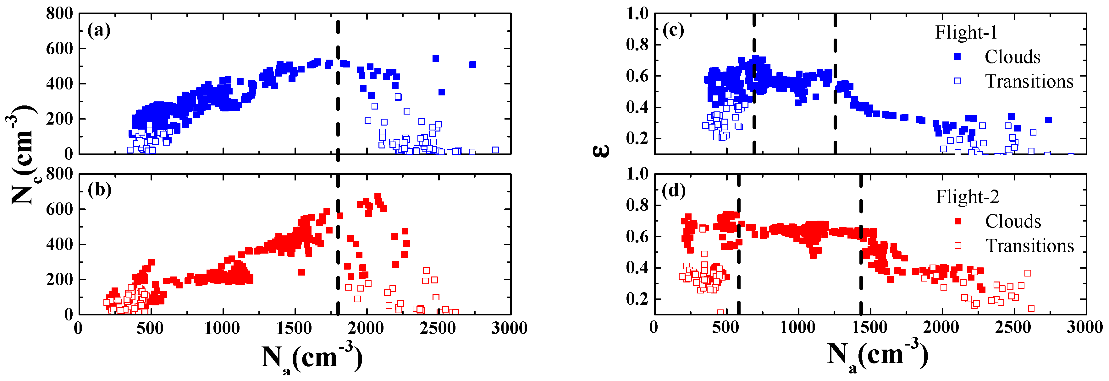
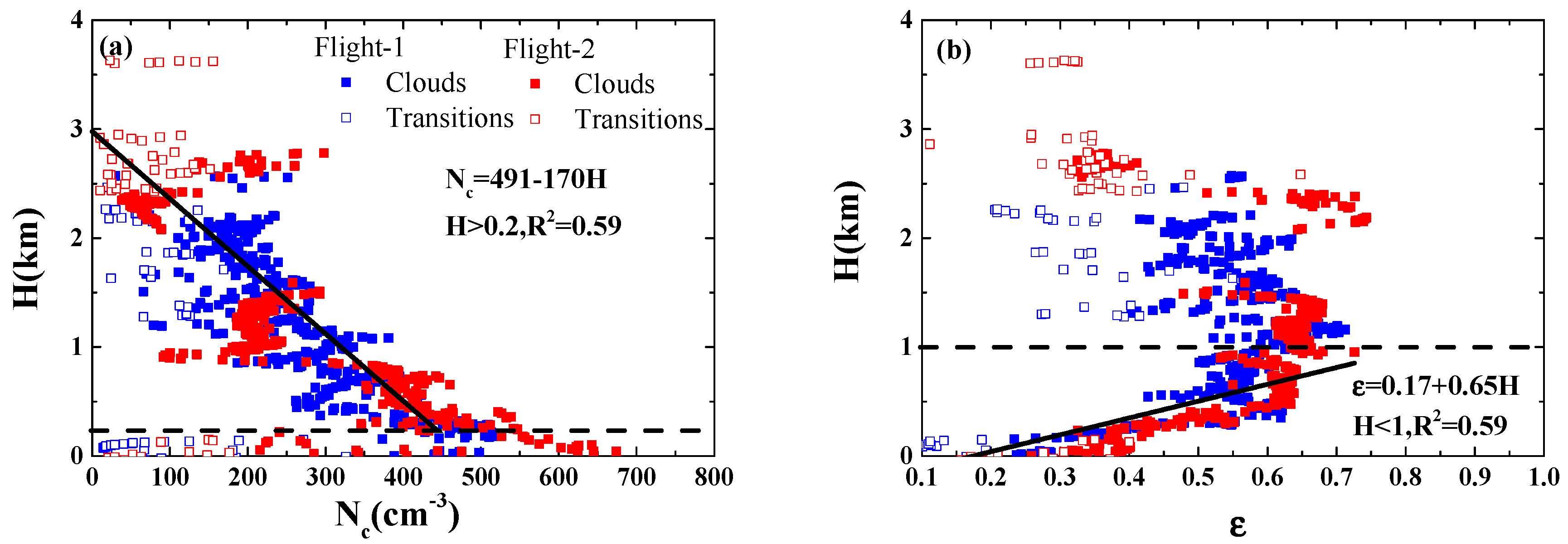
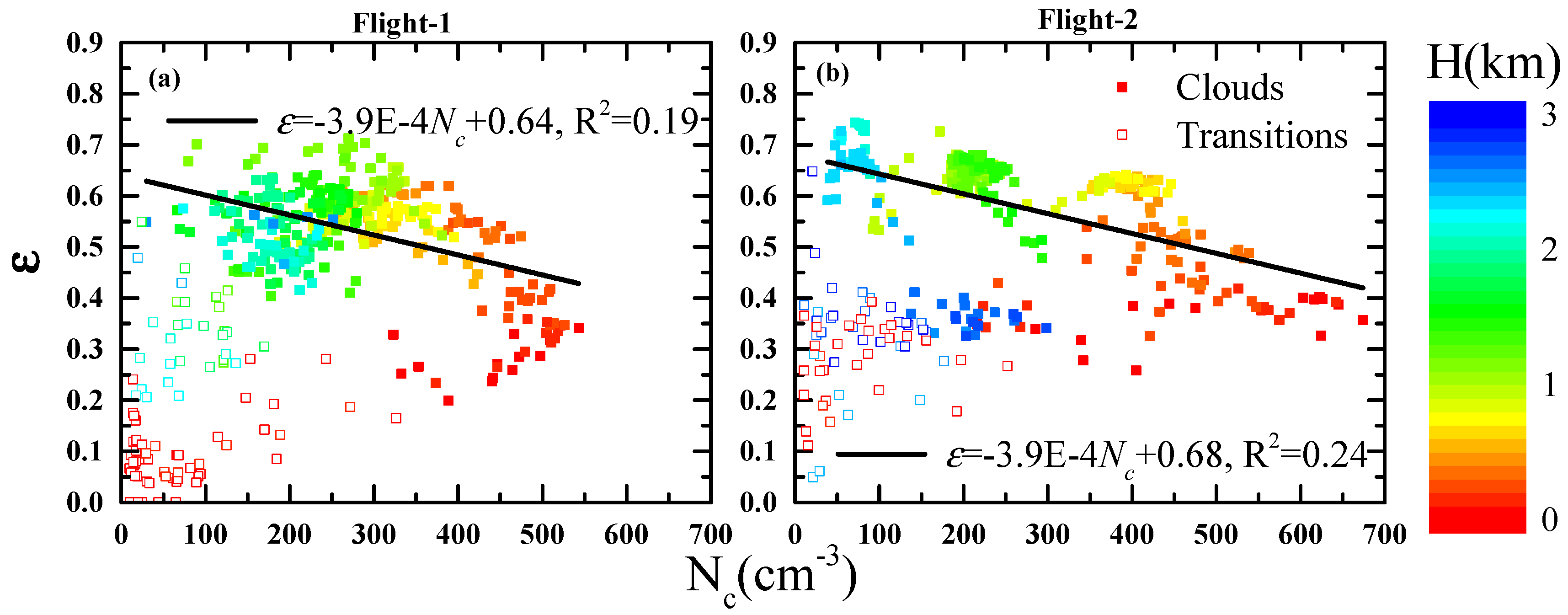
3.1. Factors Affecting $N_c$ and $\epsilon$

The nonlinear dependences of $N_c$ and $\epsilon$ on $N_a$ and w have been examined from simulation studies [34,35]. Reutter et al. [34] classified the nonlinear relationship between $N_c$ and $N_a$ into three distinct regimes according to the ratio of w/$N_a$: the aerosol-limited regime, transitional regime, and updraft-limited regime; for a fixed w, $N_c$ increases linearly with $N_a$ in the aerosol-limited regime, increases slowly in the transitional regime, and plateaus in the updraft-limited regime. Chen et al. [35] extended that work to consider the regime dependence of both $N_c$ and ε, and found for a fixed w, ε increases with $N_a$ in the aerosol-limited regime, peaks in the transitional regime, and decreases in the updraft-limited regime. However, these regime dependences of the dispersion effect were revealed using parcel model simulations and have not been verified systematically by observations.

To fill this gap, the 655 CDSDs and 146 transitional CDSDs collected during the two flights are analyzed. Figure 2 shows $N_c$ and ε as functions of $N_a$. Evidently, $N_c$ increases linearly with $N_a$ when $N_a$ is low, and increases slowly and even decreases when $N_a$ is high. In the regime of high values of $N_a$, the limited moisture is competed by abundant aerosols, leading to deactivation and decreasing $N_c$ [36]. The ε first increases with $N_a$ (the change rates of ε−$N_a$ are 0.03 and 0.06 per 100 cm⁻³ with the P values less than 0.01 for the first and second flights, respectively), peaks at certain $N_a$, and then decreases with further increase in $N_a$. These observations are highly consistent with the simulation results by Chen et al. [35], although vertical velocity was not measured.

In addition, the increasing and decreasing trends of ε vs $N_a$, and the decreasing trend of $N_c$ vs. $N_a$ at high $N_a$ are more significant when the 146 samples of transitions between environment and clouds are included, as shown in Figure 2. The distributions of ε and $N_c$ in the transitions can be explained as follows. Due to the height of detection from low to high by the aircraft and the decrease in $N_a$ as altitude increases (Figure 1), the aircraft passed through the clouds with high $N_a$ at low altitude and out of the clouds with low $N_a$ at high altitude. Therefore, the transitions generally correspond to the high and low values of $N_a$ (no medium values). Limited by the criterion of LWC less than 0.01 gm⁻³, there are almost no cloud droplets with radii greater than 5.5 μm in transitions, as shown in

Table 2. The number concentration ratios of the small droplets with radii from 1 to 5.5 μm to all droplets ($n/N_c)$ and dispersion ($\epsilon$), in the transitions and clouds, respectively.

Samples	$\mathit{n}/{\mathit{N}}_{\mathit{c}}$$\mathbf{and} \mathit{\epsilon }$
	Flight-1	Flight-2
Transitions	99% and 0.18	99% and 0.30
Clouds	88% and 0.53	81% and 0.58

. The high ratio of small droplets results in the low ε, according to the conclusion in Section 3.3. Meanwhile, the transitions at low altitude correspond to high $N_a$, and a fierce vying for water vapor in this region leads to the decreasing $N_c$.

Different heights mean different condensation growth times corresponding to different CDSDs. As Chen et al. [35] pointed out, it is worthwhile examining the height dependence of the aerosol to cloud interaction regime, and thereby, we discuss the impact of height on microphysical quantities to highlight the impact of aerosol concentration based on observations. As shown in Figure 3, $N_c$ decreases steadily with height above 0.2 km, and ε increases up to 1 km above cloud-base, while there is a weak correlation between ε and height with increasing height above 1 km. These behaviors depend on the supersaturation changes with height. For a constant value of moisture in cloud-base, the smaller value of w/$N_a$ leads to the smaller supersaturation, after the parcel rising the same height. In the updraft-limited regime, the limited moisture is competed by superabundant aerosols, leading to deactivation and decreasing $N_c$ [36]. In addition, apart from the well-known “condensational narrowing” of CDSD [42], “condensational broadening” is found up to 1 km above cloud-base in our observations. Chen et al. [36] explained this phenomenon using parcel model simulation. In the updraft-limited regime and during the initial stage of condensation growth, the parcel supersaturation ($S_p$) is low and comparable with the particle equilibrium supersaturation ($S_k$), and therefore the growth rate of the radius depends on the value of $S_p-S_k$. The larger droplets grow faster than the smaller ones owing to the dependence of $S_k$ on droplet size (see appendix in [35]), leading to the “condensational broadening”. Therefore, the observations are also in line with the simulations of the vertical profiles on microphysical parameters of the cloud by Chen et al. [36]. In addition, we examine the radius range where condensation broadening can occur according to Equation (4),

$$\frac{d\left(dr/dt\right)}{dr}=-\frac{1}{rG}\left[\frac{S_p-S_k}{r}+\frac{d{S}_k}{dr}\right]$$

(4)

where r is the radius of the droplet, t is the time, and G is a function of temperature, pressure, and so on, and the details are shown in Chen et al. [35,36]. When d(dr/dt)/dr is positive, dr/dt increases as r increases, which means that condensation broadening occurs. Assuming that the aerosol is all composed by ammonium sulfate, the radius of dry aerosol is 0.1 μm and the conditions of environment (temperature: 283.15 K, relative humidity: 0.95 and pressure: 919 hPa) are similar to the setting in Chen et al. [35,36], it is found when $S_p$ is 0.01, condensation broadening can occur at the whole radius range. With the increasing $S_p$, the radius range with condensation broadening narrows and moves toward to small droplets. When $S_p$ is 0.06, condensation broadening can occur only at the range of radius less than 4 μm.

The microphysical characteristics of the cloud are influenced by other factors as well, such as entrainment, meteorological factors, aerosol chemical component, vertical velocity in clouds, and so on. In this section, we focus on the effects of aerosol concentration and condensation on ε of CDSD and discuss two new observational phenomena, which match the latest simulations by Chen et al. [35,36]. However, considering that $N_a$ and condensation have combined effects on ε change, it is difficult to quantify their individual effects with the current data.

In addition, aerosol data were not available in many previous studies (e.g., references [9,19,43]), and the dispersion effect was discussed using the relationship between ε and $N_c$. However, in essence, the dispersion effect is the change of the CDSD shape with $N_a$, which in turn changes the optical characteristics of clouds. As shown in Figure 4, the range of ε is large when $N_c$ is low, and it narrows gradually with increasing $N_c$. There is no significant correlation between ε and $N_c$. Such a phenomenon is consistent with Zhao et al. [19]. It may be noted that the transitions correspond to both small values of ε and $N_c$ as analyzed above, and ε tends to decrease with the increasing $N_c$ in clouds, as shown in Figure 4. Therefore, the similar negative relationship between ε and $N_c$ in clouds may be also found in the study of Zhao et al. [19], if a more rigorous criterion for clouds (including the double restriction of $N_c$ and LWC) was applied. Because aerosol observation is available in this field campaign, the relationship between ε and $N_a$ is shown in Figure 2c,d, after correcting the PCASP data. Obviously, there is an appreciable difference between ε-$N_c$ and ε-$N_a$. The $N_a$ is divided into three ranges: lower, medium, and higher. These ranges are further divided into two parts (first flight and second flight): lower (300–700 cm⁻³ and 100–600 cm⁻³), medium (700–1250 cm⁻³ and 600–1400 cm⁻³), and higher (1250–3000 cm⁻³ and 1400–3000 cm⁻³). The observational analysis indicates a positive correlation between ε and $N_a$ in the lower $N_a$ ranges, but the correlation turns unapparent in the medium ranges, and even reversed in the higher ranges. The reason for the difference between ε−$N_c$ and ε−$N_a$ is that $N_c$ does not increase monotonically with $N_a$, and $N_c$ has peaks of 542 and 656 cm⁻³ for the first and second flight, respectively, when $N_a$ is about 1800 cm⁻³, as shown in Figure 2a,b. Therefore, when the observation of $N_a$ is available, it is suggested that ε−$N_a$ instead of ε−$N_c$ is used in future studies of the dispersion effect.

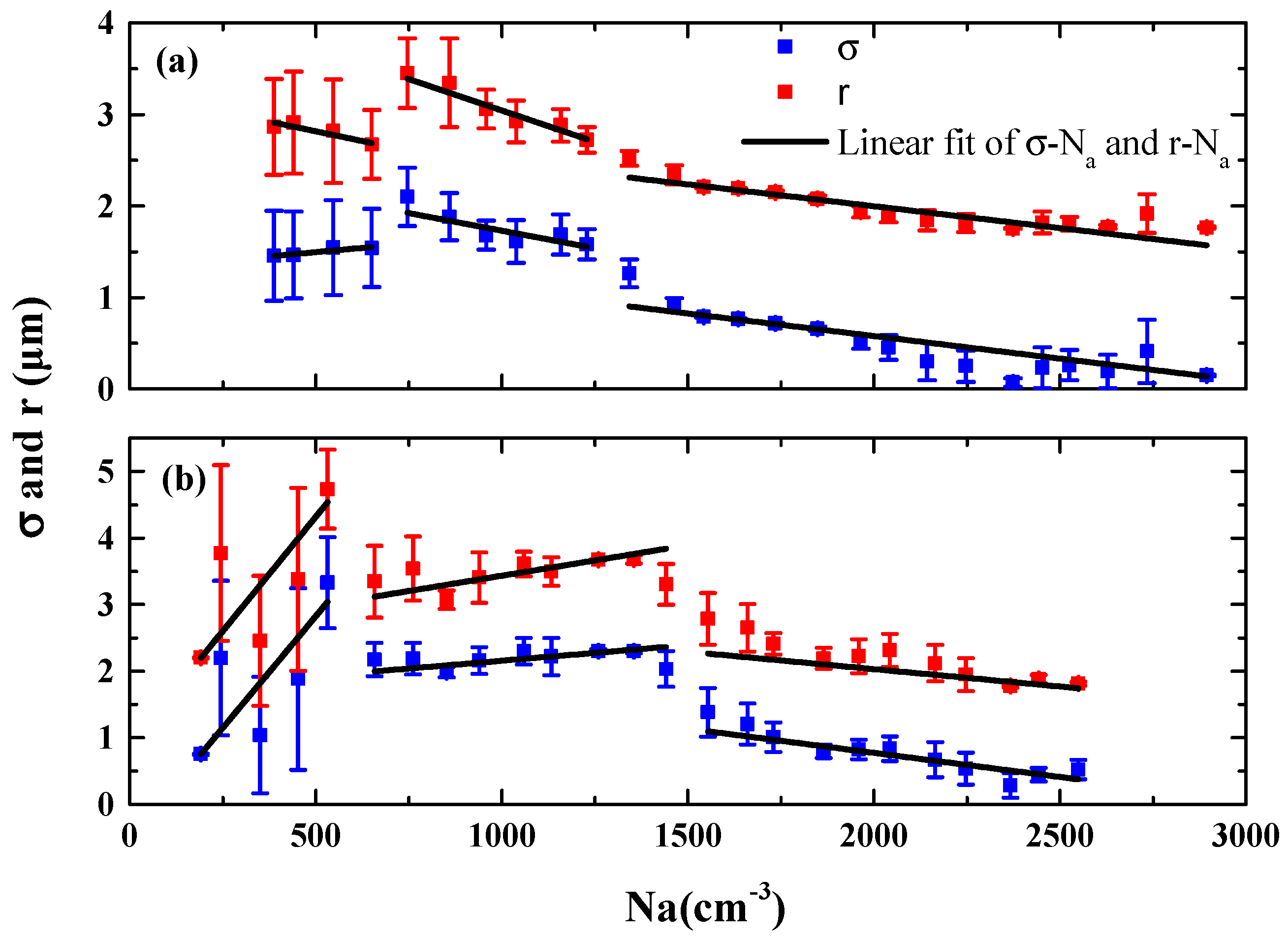
3.2. Effects of Standard Deviation and Mean Radius on ε

Because $\epsilon$ is defined as the ratio of standard deviation ($\sigma$) to mean radius ($r$) of CDSD, it would be interesting to examine the variations of σ and r with increasing $N_a$. As shown in Figure 5, $\sigma$ and $r$ vary simultaneously, and the linear fitting shows the relationship as $\sigma =0.97r-1.31$ with an R-squared of 0.93. Guo et al. [44] determined the $\epsilon$ change with entrainment rate ($\lambda$) by comparing the changes of $\sigma$ and $r$ with $\lambda$. Referring to the analysis method in Guo et al. [44], the changes of $\sigma$ and $r$ with $N_a$ (Δσ/Δ$N_a$ and Δr/Δ$N_a$, respectively), i.e., the slopes of linear fitting (k_σ and k_r, respectively), are first compared in the above-mentioned $N_a$ ranges (lower, medium, and higher) to determine the $\epsilon$ change with $N_a$. Guo et al. [44] presented that as $\lambda$ increases, σ decreases more quickly than r and thus ε tends to decrease. However, this mathematical relationship is not always valid. As shown in Figure 6 and

Table 3. The slopes of the standard deviation (k_σ) and mean radius (k_r) of CDSD with aerosol concentration ($N_a$), and the ratios of k_σ/σ and k_r /r in different $N_a$ ranges, which corresponds to different change trends of dispersion ($\epsilon$). The +, =, and - indicate an increase, invariant, and decrease of the $\epsilon$ change, respectively.

	Flight-1			Flight-2
$N_a$ (cm−3)	300–700 *	700–1250	1250–3000	100–600	600–1400	1400–3000
kσ (μm(100 cm−3)−1)	0.038	−0.096	−0.061	0.513	0.028	−0.117
kr (μm(100 cm−3)−1)	−0.080	−0.152	−0.043	0.492	0.055	−0.109
kσ/σ ((100 cm−3)−1)	0.025	−0.055	−0.123	0.279	0.013	−0.141
kr /r ((100 cm−3)−1)	−0.028	−0.050	−0.076	0.149	0.016	−0.049
$\epsilon$	+	=	-	+	=	-

*: p values are 0.068 and 0.074 for fitting lines of σ−$N_a$ and r−$N_a$, respectively. The other p values are all less than 0.05.

, the weaker decrease of $\sigma$ (−0.096 μm(100 cm⁻³)⁻¹) compared to that of $r$ (−0.152 μm(100 cm⁻³)⁻¹) leads to an invariable $\epsilon$ rather than an increasing $\epsilon$, in the medium $N_a$ range (first flight). In addition, the almost equal decrease of $\sigma$ (−0.117 μm(100 cm⁻³)⁻¹) and $r$ (−0.109 μm(100 cm⁻³)⁻¹) corresponds to the obviously decreasing $\epsilon$, in the higher $N_a$ range (second flight). The difference between the observation and the mathematical relationship is ascribed to the inaccurate analysis method. Taking the logarithm of the definition of $\epsilon$ and further differentiating it over $N_a$ yields:

$$\frac{\raisebox{1ex}{$\Delta \epsilon $}\!\left/ \!\raisebox{-1ex}{$\Delta N_{\mathrm{a}}$}\right.}{\epsilon }=\frac{\raisebox{1ex}{$\Delta \sigma $}\!\left/ \!\raisebox{-1ex}{$\Delta N_{\mathrm{a}}$}\right.}{\sigma }-\frac{\raisebox{1ex}{$\Delta r$}\!\left/ \!\raisebox{-1ex}{$\Delta N_{\mathrm{a}}$}\right.}{r}=\frac{k_{\sigma }}{\sigma }-\frac{k_r}{r}$$

(5)

It is the difference between $k_{\sigma }/\sigma$ and $k_r/r$ rather than $k_{\sigma }$ and $k_r$ that dominates in contributing to $\epsilon$ change. Only when $\sigma$ and $r$ are comparable, then using $k_{\sigma }$ and $k_r$ is equivalent to using $k_{\sigma }/\sigma$ and $k_r/r$.

As shown in Table 3, when the ratio of $k_{\sigma }/\sigma$ is approximately equal to $k_r/r$, $\epsilon$ is invariant, in the medium $N_a$ ranges in both flights. In the higher $N_a$ ranges, the ratio of $k_{\sigma }/\sigma$ is less than $k_r/r$, leading to a decreasing $\epsilon$. In addition, when the ratio of $k_{\sigma }/\sigma$ is greater than $k_r/r$, $\epsilon$ is increased, in the lower $N_a$ range for the second flight. Although the P value is larger than 0.05 in the lower $N_a$ range for the first flight, the conclusion is consistent with other $N_a$ ranges. Therefore, by comparing $k_{\sigma }/\sigma$ and $k_r/r$ at multiple $N_a$ ranges, the change trend of $\epsilon$ can be obtained.

Although $\epsilon$ increases first and then decreases in both two cases, the reasons are different, especially in the stages of $\epsilon$ increasing and remaining invariable. As shown in Figure 6 and Table 3, $\epsilon$ increases with $N_a$ in the lower $N_a$ ranges with positive $k_{\sigma }$ in both flights and opposite signs of $k_r$. When $\epsilon$ is invariable in the medium $N_a$ ranges, both k_σ and k_r are negative in the first flight but positive in the second flight. The differences may be attributed to w in clouds because the microphysical parameters of clouds are affected not only by $N_a$ but also by w. Due to the simultaneous influences of $N_a$ and w, the difference in Figure 6 could occur in different $w-N_a$ combinations in the two flights.

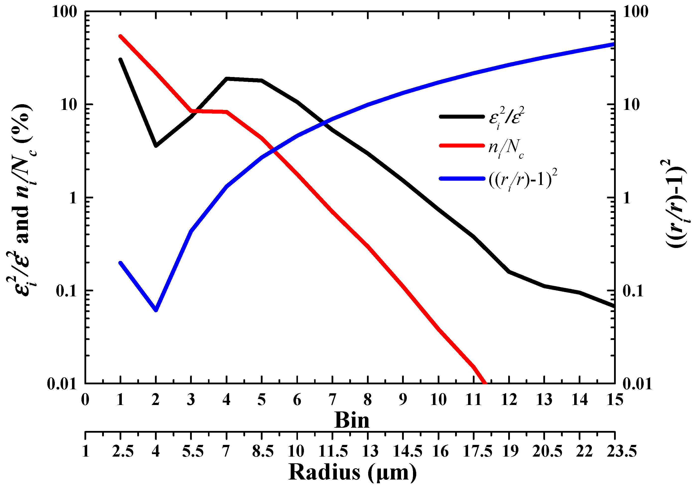
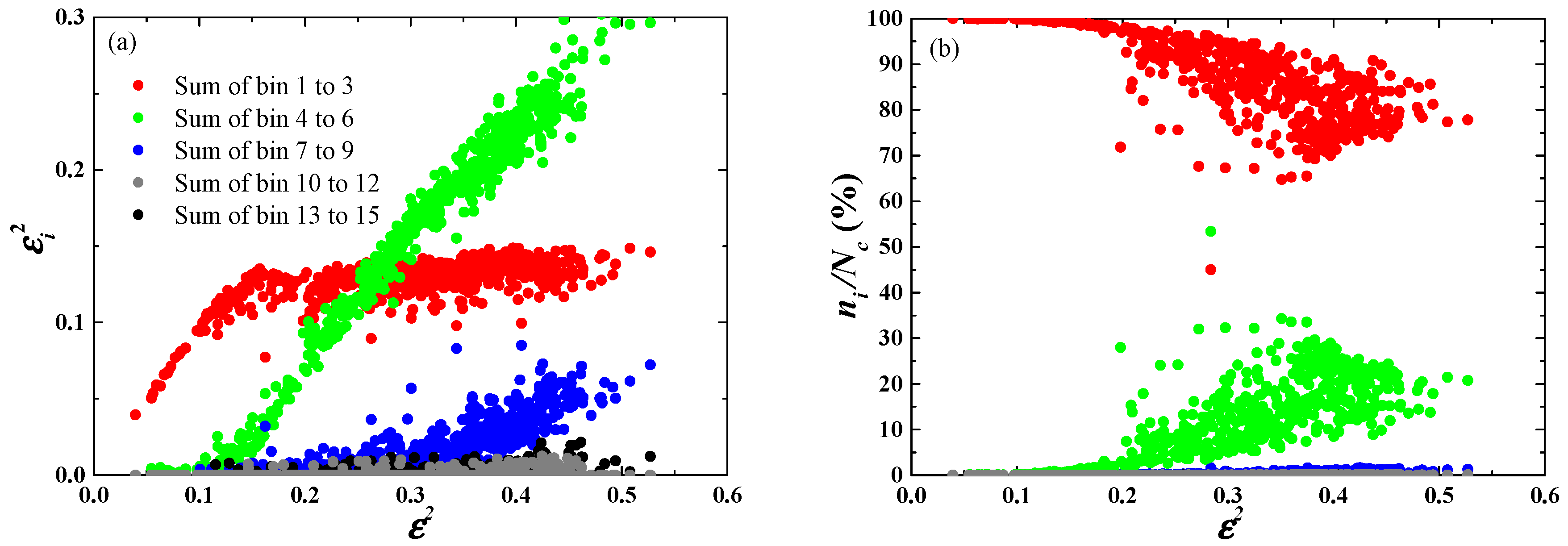
3.3. Contributions of Droplets of Different Sizes to ε

The values of ε can be viewed not only as the combined effects of σ and r, but also as the combined effects of droplets of different sizes. A new algorithm is proposed to quantify the contributions of cloud droplets in different size ranges to $\epsilon$; the derivation of the algorithm is shown in Section 2.2. Obviously, the contribution ratio of ${\epsilon }^2$ caused by each bin to ${\epsilon }^2$ of the CDSD (${\epsilon }_i^2/{\epsilon }^2$) is dominated by two factors including the relative deviation of mean radius (${\left(\frac{r_i}{r}-1\right)}^2$) and the concentration ratio ($n_i/N_c$), as shown in Equation (3). The above three variables are quantified for the 15 bins with 655 CDSDs, and the result is shown in Figure 7. As the bin number increases, the ${\epsilon }_i^2/{\epsilon }^2$ first decreases in the first two bins, next increases in the 3rd and 4th bins, then decreases again in the last 11 bins. The main contributors to ${\epsilon }^2$ are the first six bins with a total ratio of 88.7%, and the contributions of small droplets with bins 1 to 3 and medium droplets with bins 4 to 6 are comparable. According to the statistics of mean radii of the 655 CDSDs, the frequency distributions of the mean radius in the 1st, 2nd, and 3rd bins are 17%, 72%, and 11%, respectively. Hence, the three bins correspond to small ${\left(\frac{r_i}{r}-1\right)}^2$, but the extremely high values of $n_i/N_c$ lead to the large ${\epsilon }_i^2/{\epsilon }^2$ in the first three bins.

Based on the above analysis, we further examine which part of the CDSD dominates the $\epsilon$ change. The CDSD is divided equally into five size ranges: 1 to 5.5 μm (sum of the first three bins), 5.5 to 10 μm (sum of bins 4 to 6), 10 to 14.5 μm (sum of bins 7 to 9), 14.5 to 19 μm (sum of bins 10 to 12), and 19 to 23.5 μm (sum of the last three bins). With the increase of ${\epsilon }^2$, the contribution values of droplets of different size-ranges to ${\epsilon }^2$ (${\epsilon }_i^2$) are shown in Figure 8a. It is found that the main contributors to the change of ${\epsilon }^2$ are different at the different ranges of ${\epsilon }^2$. The equations of linear fitting of ${\epsilon }_i^2$ and ${\epsilon }^2$ at different ranges of ${\epsilon }^2$ are summarized in

Table 4. The linear fitting of ${\epsilon }_i^2$ and ${\epsilon }^2$ at different ranges of ${\epsilon }^2$.

ε	ε2	Bins 1–3	Bins 4–6	Bins 7–9	$\mathbf{Dominators} \mathbf{for} \mathit{\epsilon } \mathbf{Changes}$
ε$\le$0.32	ε2$\le$0.1	${\epsilon }_i^2$ = 0.98ε2	-	-	Bin 1–3
0.32$<$ε $\le$ 0.4	0.1$<$ ε2$\le$0.16	${\epsilon }_{i }^2$ = 0.54ε2 + 0.04	${\epsilon }_i^2$ = 0.41ε2 − 0.04	-	Bin 1–6
0.4 $<$ ε$\le$0.55	0.16$<$ε2$\le$0.3	-	${\epsilon }_i^{2 }$= 0.9ε2 − 0.11	-	Bin 4–6
ε$>$0.55	ε 2$>$0.3	-	${\epsilon }_i^{2 }$= 0.62ε2 − 0.02	${\epsilon }_i^2$ = 0.29ε2 − 0.08	Bin 4–9

- means the slope of the line is less than 0.1.

. The slopes of these fitting lines demonstrate the importance of ${\epsilon }_i^2$ for ${\epsilon }^2$ change.

As shown in Figure 8 and Table 4, when ${\epsilon }^2$ is less than 0.1, i.e., $\epsilon$ is less than 0.32, the droplets of only bins 1 to 3 dominate the change of ${\epsilon }^2$, and there are almost no cloud droplets with radii greater than 5.5 μm. When ${\epsilon }^2$ is between 0.1 and 0.16, i.e., $\epsilon$ is between 0.32 and 0.4, the change of ${\epsilon }^2$ is dominated by the droplets of bins 1 to 6, and the $n_i/N_c$ of droplets with radii from 5.5 to 10 μm is between 0.1% and 1%. When ${\epsilon }^2$ is greater than 0.16, i.e., $\epsilon$ is greater than 0.4, the droplets of bins 1 to 3 have almost no effect on the change of ${\epsilon }^2$. When ${\epsilon }^2$ is between 0.16 and 0.3, i.e., $\epsilon$ is between 0.4 and 0.55, the change of ${\epsilon }^2$ is almost dominated by the droplets of bins 4 to 6, and the $n_i/N_c$ of these droplets is between 1% and 10%. When ${\epsilon }^2$ is greater than 0.3, i.e., $\epsilon$ is greater than 0.55, the droplets of bins 7 to 9 begin to affect the change of ${\epsilon }^2$, but the droplets of bins 4 to 6 have the larger effect on the change of ${\epsilon }^2$ than other size ranges of droplets. At this stage, the $n_i/N_c$ of droplets with radii from 5.5 to 10 μm is between 5% and 30% and that of droplets with radii from 10 to 14.5 μm is between 0.1% and 1%. Due to the extremely low $n_i/N_c$ of the larger droplets (less than 0.1%), the droplets with radii from 14.5 to 23.5 μm have little effect on the change of $\epsilon$ in the two flights. The decreasing $n_i/N_c$ of small droplets of bins 1 to 3 corresponds to the increasing $n_i/N_c$ of medium droplets of bins 4 to 6 as ${\epsilon }^2$ increases. Therefore, there is also a positive correlation between $n_i/N_c$ of medium droplets and the change of ${\epsilon }^2$.

In short, the small droplets with radii from 1 to 5.5 μm and the medium droplets with radii from 5.5 to 10 μm are the main contributors to $\epsilon$. The medium droplets dominate the change of $\epsilon$ as long as they are present in CDSD, corresponding to the $n_i/N_c$ of these droplets greater than 1%.

4. Conclusions

Aircraft measurements of aerosol concentrations and CDSDs including 655 non-precipitating samples in clouds and 146 transitional samples between environment and clouds were collected by employing two flights in Hebei, China, in 2015. The observations that $\epsilon$ first increases and then decreases with increasing $N_a$ and “condensational broadening” occurs up to 1 km above cloud-base are consistent with the recent simulations by Chen et al. [35,36]. However, aerosol concentration and condensation have combined effects on the change of $\epsilon$, and therefore their individual effects cannot be clearly determined. Accordingly, this study only provides potential observational evidence for the numerical simulations [35,36]. In addition, we recommend that the focus should be shifted from $\epsilon$−$N_c$ to $\epsilon$−$N_a$ in future research on the dispersion effect, when details of $N_a$ are available.

Because $\epsilon$ is defined as the ratio of $\sigma$ to $r$, the variations of $\sigma$ and $r$ with $N_a$ were examined in different ranges of $N_a$. It is found that the variation of $\epsilon$ with $N_a$ can be well explained by comparing $k_{\sigma }/\sigma$ and $k_r/r$ rather than by comparing $k_{\sigma }$ and $k_r$, and we derived their mathematical relationship. Specifically, when $k_{\sigma }/\sigma$ is greater than $k_r/r$, corresponding to the lower ranges of $N_a$, $\epsilon$ increases. When $k_{\sigma }/\sigma$ is approximately equal to $k_r/r$, corresponding to the medium ranges of $N_a$, $\epsilon$ is invariable. When $k_{\sigma }/\sigma$ is less than $k_r/r$, corresponding to the higher ranges of $N_a$, $\epsilon$ decreases. Therefore, $\epsilon$ exhibits a trend of first increasing and then decreasing over the entire ranges of $N_a$.

In addition, we proposed a new algorithm to quantify the contributions of droplets of different size ranges to $\epsilon$. The major contributors to $\epsilon$ are the small droplets with radii of 1 to 5.5 μm and the medium droplets with radii of 5.5 to 10 μm with a total contribution ratio of 88.7%, and their contributions are comparable. When $\epsilon$ is less than 0.32, $\epsilon$ is mostly contributed to by the small droplets with radii of 1 to 5.5 μm. The medium droplets with radii of 5.5 to 10 μm dominate the change of $\epsilon$ as long as they are present in CDSD, corresponding to the number concentration ratio of these droplets to all droplets is greater than 1%.

The aerosol-cloud interactions are dominated by both aerosol concentration and vertical velocity. Due to the lack of vertical velocity observations, the regime of aerosol-cloud interactions was only estimated by the aerosol concentration to discuss the observational phenomena in this study. It may be noted that the vertical velocity must show vertical variance, rather than constant in clouds, which causes the uncertainty between the aerosol effect and the vertical velocity effect on $\epsilon$ and $N_c$ in this study. In other words, the relationship between $N_a$ and (also between $N_a$ and $N_c$) might not necessarily reflect the aerosol indirect effect because only two flights are analyzed. More data will be analyzed to further study this topic. Therefore, the observed data with wide ranges of aerosol concentration and vertical velocity should be analyzed comprehensively in future research to fully confirm the results reported in Chen et al. [35,36].

References

1. Ramanathan, V.; Crutzen, P.J.; Kiehl, J.T.; Rosenfeld, D. Aerosols, climate, and the hydrological cycle. Science 2001, 294, 2119–2124. [Google Scholar] [CrossRef] [PubMed]
2. Rosenfeld, D.; Lohmann, U.; Raga, G.B.; ODown, C.D.; Kulmala, M.; Fuzzi, S.; Reissell, A.; Andreae, M.O. Flood or drought: How do aerosols affect precipitation? Science 2008, 321, 1309–1313. [Google Scholar] [CrossRef] [PubMed]
3. Koren, I.; Dagan, G.; Altaratz, O. From aerosol-limited to invigoration of warm convective clouds. Science 2014, 344, 1143–1146. [Google Scholar] [CrossRef] [PubMed]
4. Quaas, J. Approaches to Observe Anthropogenic Aerosol-Cloud Interactions. Curr. Clim. Chang. Rep. 2015, 1, 297–304. [Google Scholar] [CrossRef] [PubMed] [Green Version]
5. Haywood, J.; Boucher, O. Estimates of the direct and indirect radiative forcing due to tropospheric aerosols: A review. Rev. Geophys. 2000, 38, 513–543. [Google Scholar] [CrossRef] [Green Version]
6. Twomey, S. Pollution and the planetary albedo. Atmos. Environ. 1974, 8, 1251–1256. [Google Scholar] [CrossRef]
7. Twomey, S. The Influence of Pollution on the Shortwave Albedo of Clouds. J. Atmos. Sci. 1977, 34, 1149–1152. [Google Scholar] [CrossRef] [Green Version]
8. Zhao, C.; Zhao, L.; Dong, X. A Case Study of Stratus Cloud Properties Using in Situ Aircraft Observations over Huanghua, China. Atmosphere 2019, 10, 19. [Google Scholar] [CrossRef]
9. Liu, Y.; Daum, P.H. Anthropogenic aerosols. Indirect warming effect from dispersion forcing. Nature 2002, 419, 580–581. [Google Scholar] [CrossRef] [PubMed]
10. Intergovernmental Panel on Climate Change. Climate Change 2013: The Physical Science Basis. Contribution of Working Group I to the Fifth Assessment Report of the Intergovernmental Panel on Climate Change; Cambridge Univ. Press: Cambridge, UK, 2013; p. 1535. [Google Scholar]
11. Quaas, J.; Boucher, O.; Lohmann, U. Constraining the total aerosol indirect effect in the LMDZ and ECHAM4 GCMs using MODIS satellite data. Atmos. Chem. Phys. 2006, 6, 947–955. [Google Scholar] [CrossRef] [Green Version]
12. Ruckstuhl, C.; Norris, J.R.; Philipona, R. Is there evidence for an aerosol indirect effect during the recent aerosol optical depth decline in Europe? J. Geophys. Res. 2010, 115, 288–303. [Google Scholar] [CrossRef]
13. Xie, X.; Liu, X. Analytical studies of the cloud droplet spectral dispersion influence on the first indirect aerosol effect. Adv. Atmos. Sci. 2013, 30, 1313–1319. [Google Scholar] [CrossRef]
14. Peng, Y.; Lohmann, U. Sensitivity study of the spectral dispersion of the cloud droplet size distribution on the indirect aerosol effect. Geophys. Res. Lett. 2003, 30. [Google Scholar] [CrossRef] [Green Version]
15. Rotstayn, L.D.; Liu, Y. Sensitivity of the first indirect aerosol effect to an increase of cloud droplet spectral dispersion with droplet number concentration. J. Clim. 2003, 16, 3476–3481. [Google Scholar] [CrossRef]
16. Chen, Y.; Penner, J.E. Uncertainty analysis for estimates of the first indirect aerosol effect. Atmos. Chem. Phys. 2005, 5, 2935–2948. [Google Scholar] [CrossRef] [Green Version]
17. Tas, E.; Koren, I.; Altaratz, O. On the sensitivity of droplet size relative dispersion to warm cumulus cloud evolution. Geophys. Res. Lett. 2012, 39, 189–200. [Google Scholar] [CrossRef]
18. Lu, M.L.; Seinfeld, J.H. Effect of aerosol number concentration on cloud droplet dispersion: A large-eddy simulation study and implications for aerosol indirect forcing. J. Geophys. Res. 2006, 111. [Google Scholar] [CrossRef] [Green Version]
19. Zhao, C.; Tie, X.; Brasseur, G.; Noone, K.J.; Nakajima, T.; Zhang, Q.; Zhang, R.; Huang, M.; Duan, Y.; Li, G.; et al. Aircraft measurements of cloud droplet spectral dispersion and implications for indirect aerosol radiative forcing. Geophys. Res. Lett. 2006, 33, 373–386. [Google Scholar] [CrossRef]
20. Wang, X.; Xue, H.; Fang, W.; Zheng, G. A Study of Shallow Cumulus Cloud Droplet Dispersion by Large Eddy Simulations. Acta Meteorol. Sin. 2011, 25, 166–175. [Google Scholar] [CrossRef]
21. Ma, J.; Chen, Y.; Wang, W.; Yan, P.; Liu, H.; Yang, S.; Hu, Z.; Lelieveld, J. Strong air pollution causes widespread haze-clouds over China. J. Geophys. Res. 2010, 115, 311–319. [Google Scholar] [CrossRef]
22. Yum, S.S.; Hudson, J.G. Adiabatic predictions and observations of cloud droplet spectral broadness. Atmos. Res. 2005, 73, 203–223. [Google Scholar] [CrossRef]
23. Liu, Y.; Daum, P.H.; Yum, S.S. Analytical expression for the relative dispersion of the cloud droplet size distribution. Geophys. Res. Lett. 2006, 33, 356–360. [Google Scholar] [CrossRef]
24. Lu, C.; Niu, S.; Liu, Y.; Vogelmann, A.M. Empirical relationship between entrainment rate and microphysics in cumulus clouds. Geophys. Res. Lett. 2013, 40, 2333–2338. [Google Scholar] [CrossRef]
25. Kumar, B.; Bera, S.; Prabha, T.; Grabowski, W. Cloud-edge mixing: Direct numerical simulation and observations in Indian Monsoon clouds. J. Adv. Model. Earth Syst. 2017, 9, 332–353. [Google Scholar] [CrossRef] [Green Version]
26. Martin, G.M.; Johnson, D.W.; Spice, A. The Measurement and Parameterization of Effective Radius of Droplets in Warm Stratocumulus Clouds. J. Atmos. Sci. 1994, 51, 1823–1842. [Google Scholar] [CrossRef] [Green Version]
27. Rotstayn, L.D.; Liu, Y. Cloud droplet spectral dispersion and the indirect aerosol effect: Comparison of two treatments in a GCM. Geophys. Res. Lett. 2009, 36, 137. [Google Scholar] [CrossRef]
28. Liu, Y.; Daum, P.H.; Guo, H.; Peng, Y. Dispersion Bias, Dispersion Effect, and Aerosol-Cloud Conundrum. Environ. Res. Lett. 2008, 3, 045021. [Google Scholar] [CrossRef]
29. Mcfarquhar, G.M.; Heymsfield, A.J. Parameterizations of INDOEX microphysical measurements and calculations of cloud susceptibility: Applications for climate studies. J. Geophys. Res. 2001, 106, 28675–28698. [Google Scholar] [CrossRef] [Green Version]
30. Wood, R.; Irons, S.; Jonas, P.R. How Important Is the Spectral Ripening Effect in Stratiform Boundary Layer Clouds? Studies Using Simple Trajectory Analysis. J. Atmos. Sci. 2002, 59, 2681–2693. [Google Scholar] [CrossRef]
31. Martins, J.A.; Dias, M.A.F.S. The impact of smoke from forest fires on the spectral dispersion of cloud droplet size distributions in the Amazonian region. Environ. Res. Lett. 2009, 4, 015002. [Google Scholar] [CrossRef] [Green Version]
32. Hudson, J.G.; Noble, S.; Jha, V. Cloud droplet spectral width relationship to CCN spectra and vertical velocity. J. Geophys. Res. 2012, 117, D11211. [Google Scholar] [CrossRef]
33. Lu, C.; Liu, Y.; Niu, S.; Vogelmann, A.M. Observed impacts of vertical velocity on cloud microphysics and implications for aerosol indirect effects. Geophys. Res. Lett. 2012, 39, 21808. [Google Scholar] [CrossRef]
34. Reutter, P.; Trentmann, J.; Su, H.; Simmel, M.; Rose, D.; Gunthe, S.S.; Wernli, H.; Andreae, M.O.; Poschl, U. Aerosol- and updraft-limited regimes of cloud droplet formation: Influence of particle number, size and hygroscopicity on the activation of cloud condensation nuclei (CCN). Atmos. Chem. Phys. 2009, 9, 776–781. [Google Scholar] [CrossRef]
35. Chen, J.; Liu, Y.; Zhang, M.; Zhang, M.; Peng, Y. New understanding and quantification of the regime dependence of aerosol-cloud interaction for studying aerosol indirect effects. Geophys. Res. Lett. 2016, 43, 1780–1787. [Google Scholar] [CrossRef] [Green Version]
36. Chen, J.; Liu, Y.; Zhang, M.; Peng, Y. Height Dependency of Aerosol-Cloud Interaction Regimes. J. Geophys. Res. 2018, 123, 491–506. [Google Scholar] [CrossRef]
37. Czys, R.R. Cloud Seeding; Environmental Geology: Dordrecht, The Netherlands, 1999. [Google Scholar]
38. Chazette, P.; Randriamiarisoa, H.; Sanak, J.; Couvert, P.; Flamant, C. Optical properties of urban aerosol from airborne and ground-based in situ measurements performed during the Etude et Simulation de la Qualité de l’air en Ile de France (ESQUIF) program. J. Geophys. Res. 2005, 110, D02206. [Google Scholar] [CrossRef]
39. Zhao, C.; Qiu, Y.; Dong, X.; Wang, Z.; Peng, Y.; Li, B.; Wu, Z.; Wang, Y. Negative Aerosol-Cloud re Relationship from Aircraft Observations Over Hebei, China. Earth Space Sci. 2018, 5, 19–29. [Google Scholar] [CrossRef]
40. Kleinman, L.I.; Daum, P.H.; Lee, Y.N.; Lewis, E.R.; Sedlacek, A.J., III; Senum, G.I.; Springston, S.R.; Wang, J.; Hubbe, J.; Jayne, J.; et al. Aerosol concentration and size distribution measured below, in, and above cloud from the DOE G-1 during VOCALS-REx. Atmos. Chem. Phys. 2012, 12, 207–223. [Google Scholar] [CrossRef] [Green Version]
41. Gillani, N.V.; Schwartz, S.E.; Leaitch, W.R.; Strapp, J.W.; Isaac, G.A. Field observations in continental stratiform clouds: Partitioning of cloud particles between droplets and unactivated interstitial aerosols. J. Geophys. Res. 1995, 100, 18687–18706. [Google Scholar] [CrossRef]
42. Wallace, J.M.; Hobbs, P.V. Atmospheric Science: An Introductory Survey., 2nd ed.; Elsevier Academic Press: Cambridge, MA, USA, 2006. [Google Scholar]
43. Deng, Z.; Zhao, C.; Zhang, Q.; Huang, M.; Ma, X. Statistical analysis of microphysical properties and the parameterization of effective radius of warm clouds in Beijing area. Atmos. Res. 2009, 93, 888–896. [Google Scholar] [CrossRef]
44. Guo, X.; Lu, C.; Zhao, T.; Liu, Y.; Zhang, G.; Luo, S. Observational study of the relationship between entrainment rate and relative dispersion in deep convective clouds. Atmos. Res. 2018, 199, 186–192. [Google Scholar] [CrossRef]
Figure 1. Vertical profiles of aerosol concentration ( N a ) and liquid water content (LWC) in the two flights, corresponding to (a) and (b), respectively.
Atmosphere 10 00109 g001
Figure 2. Relationships of cloud droplet concentration ( N c ) and relative dispersion ( ε ) to aerosol concentration ( N a ) in the two flights. (a,c) and (b,d) are for the first and second flights, respectively. The vertical lines indicate the N a values where the trends of N c N a and ε N a begin to change.
Atmosphere 10 00109 g002
Figure 3. Relationships of cloud droplet concentration ( N c ) and relative dispersion ( ε ) to the height above cloud-base ( H ), corresponding to (a) and (b), respectively.
Atmosphere 10 00109 g003
Figure 4. Relationship between cloud droplet concentration ( N c ) and relative dispersion ( ε ). The color scheme denotes the height above the cloud base (H). The black lines are linear fittings of ε N c in clouds. (a) and (b) are for the first and second flights, respectively.
Atmosphere 10 00109 g004
Figure 5. Relationship between standard deviation (σ) and mean radius ( r ) of cloud droplet size distribution.
Atmosphere 10 00109 g005
Figure 6. Standard deviation (σ) and mean radius (r) of cloud droplet size distribution vs aerosol number concentrations ( N a ). The black lines are linear fittings of σ− N a and r− N a in the three ranges of N a . (a) and (b) are for the first and second flights, respectively.
Atmosphere 10 00109 g006
Figure 7. The relationship between ε i 2 / ε 2 and bins of CDSD as well as that between n i / N c and bins, and ( r i r 1 ) 2 and bins, where the ε,   N c , and r represent the dispersion, number concentration, and mean radius of CDSD.
Atmosphere 10 00109 g007
Figure 8. Contribution values to ε 2 ( ε i 2 ) and number concentration ratios ( n i / N ) of different size ranges of droplets at different ε 2 , corresponding to (a) and (b), respectively.
Atmosphere 10 00109 g008