Anthropogenic and Natural Factors Affecting Trends in Atmospheric Methane in Barrow, Alaska


Abstract
:1. Introduction
2. Results and Discussion
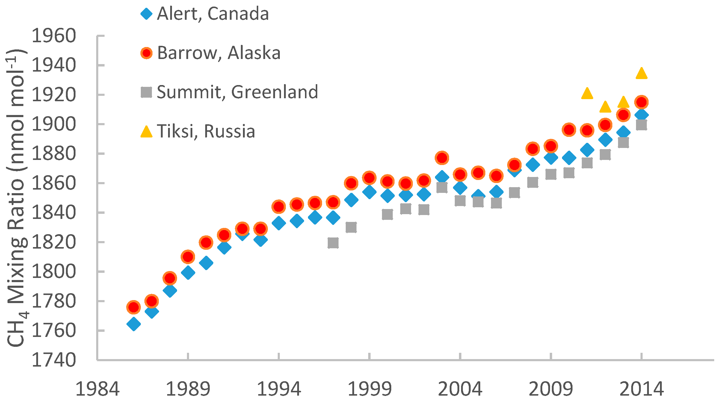
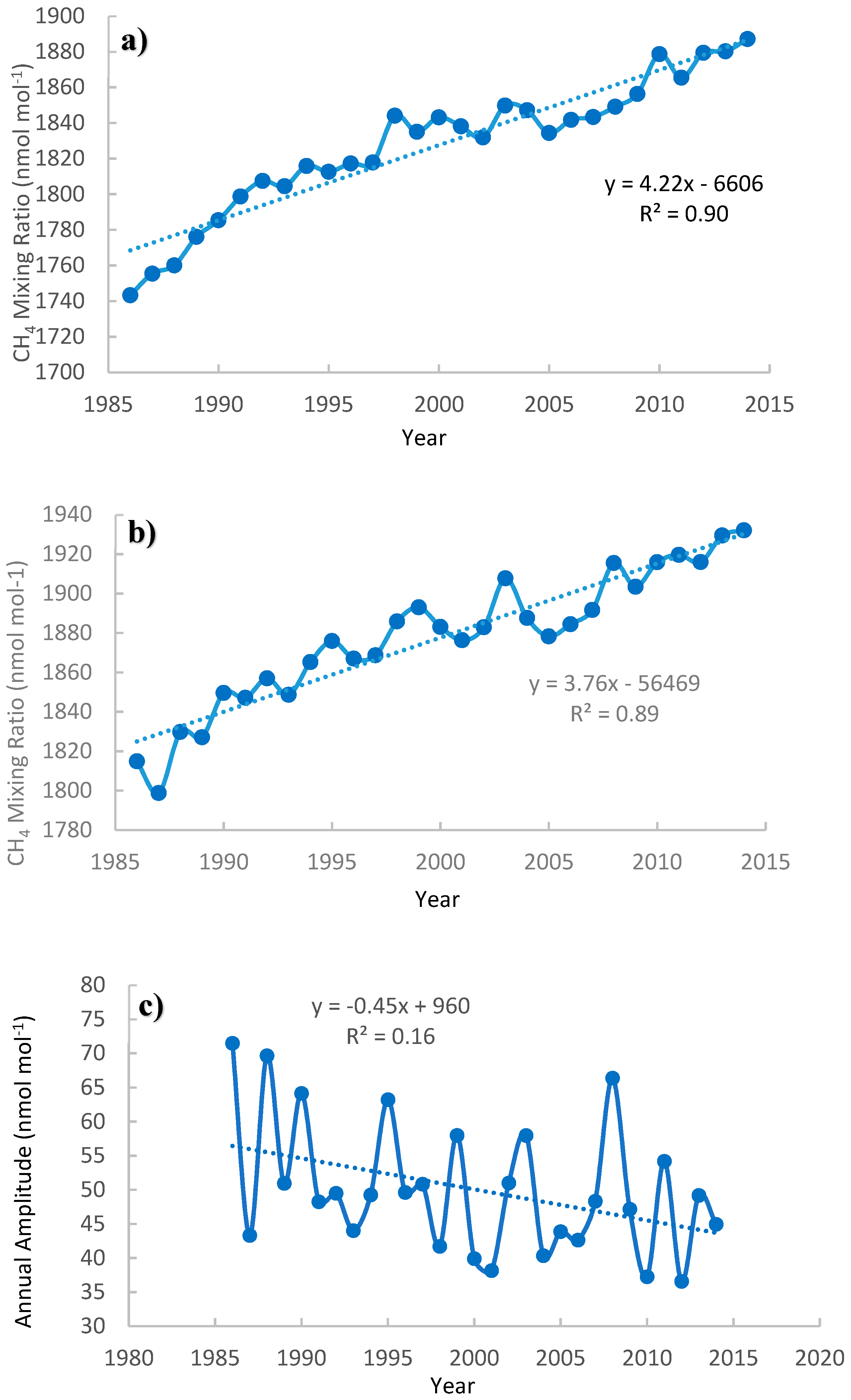
2.1. General Characteristics
2.2. Regional Anthropogenic Influences
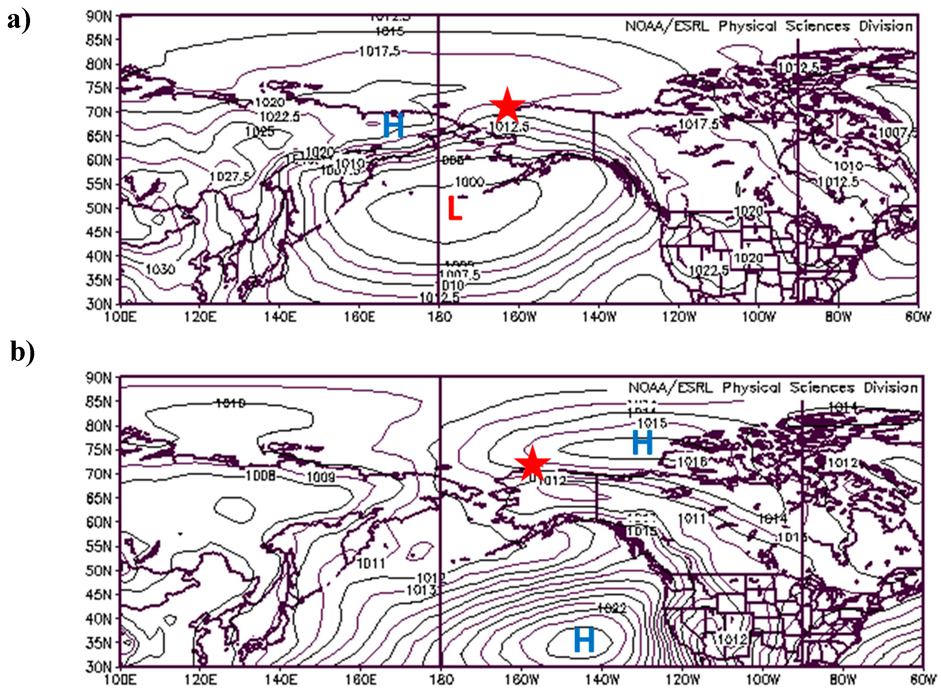
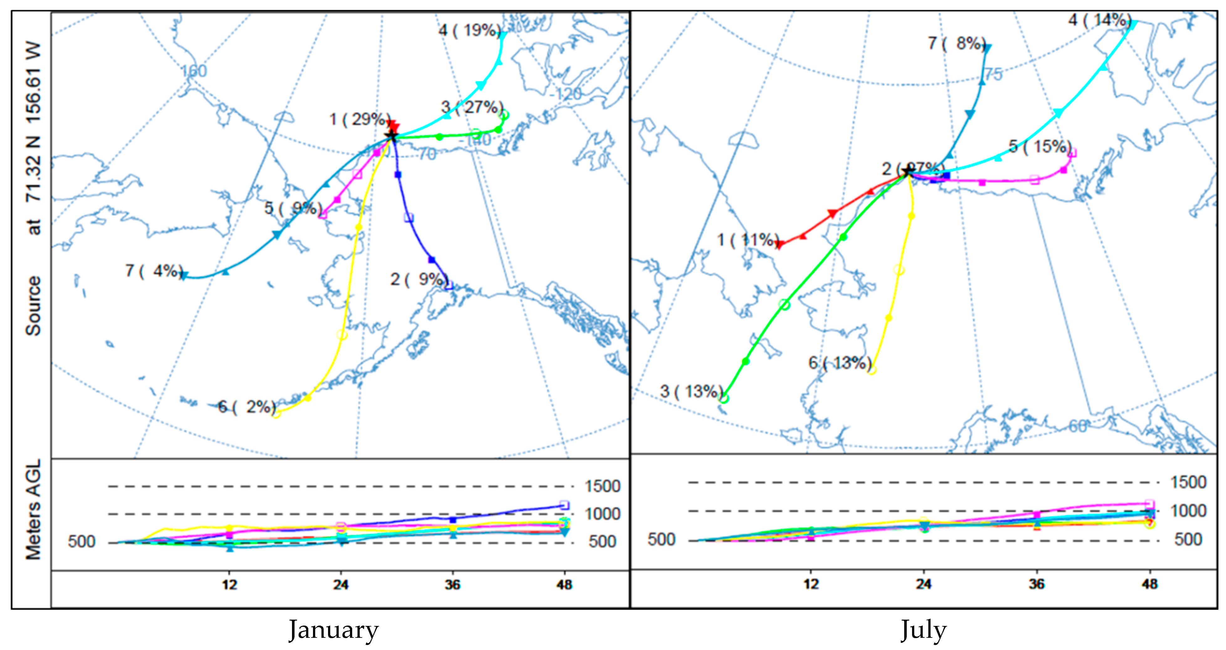
2.3. Transport
2.4. Influence of Wetland Emissions During Warm Seasons
3. Data and Methods
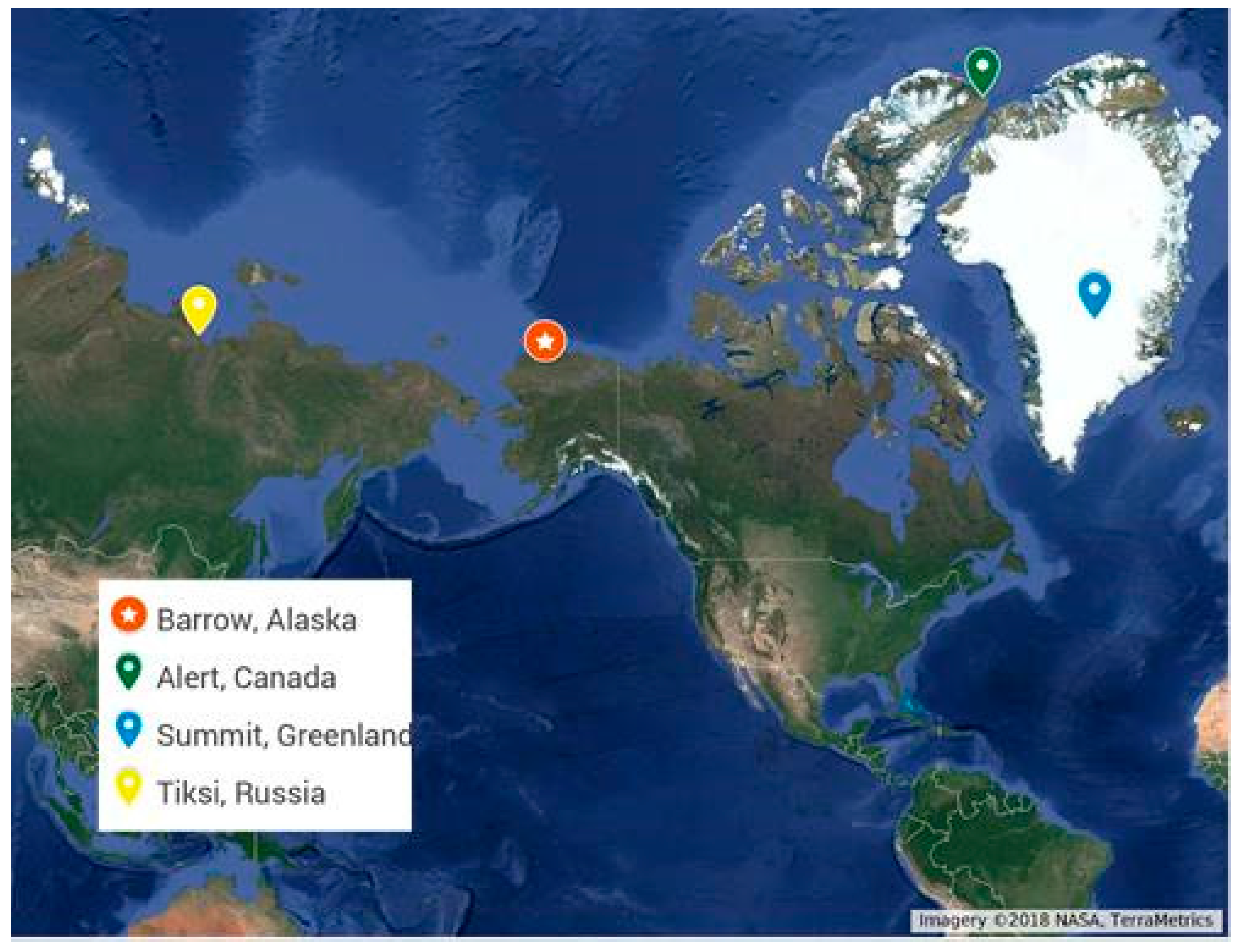
3.1. Site Locations
3.2. Data
3.3. Trajectory Simulations
3.4. Rate of Oxidation, Dilution Factor, and Wetland Flux Estimation
4. Summary
Supplementary Materials
Author Contributions
Funding
Acknowledgments
Conflicts of Interest
References
- World Meteorological Organization WMO Greenhouse Gas Bulletin. Available online: https://library.wmo.int/opac/doc_num.php?explnum_id=4022 (accessed on 31 May 2018).
- Dlugokencky, E.J.; Bruhwiler, L.; White, J.W.C.; Emmons, L.K.; Novelli, P.C.; Montzka, S.A.; Masarie, K.A.; Lang, P.M.; Crotwell, A.M.; Miller, J.B.; et al. Observational constraints on recent increases in the atmospheric CH4 burden. Geophys. Res. Lett. 2009, 36. [Google Scholar] [CrossRef]
- Nisbet, E.G.; Dlugokencky, E.J.; Manning, M.R.; Lowry, D.; Fisher, R.E.; France, J.L.; Michel, S.E.; Miller, J.B.; White, J.W.C.; Vaughn, B.; et al. Rising atmospheric methane: 2007–2014 growth and isotopic shift. Glob. Biogeochem. Cycles 2016, 30, 1356–1370. [Google Scholar] [CrossRef]
- Kai, F.M.; Tyler, S.C.; Randerson, J.T.; Blake, D.R. Reduced methane growth rate explained by decreased Northern Hemisphere microbial sources. Nature 2011, 476, 194–197. [Google Scholar] [CrossRef] [PubMed]
- Kirschke, S.; Bousquet, P.; Ciais, P.; Saunois, M.; Canadell, J.G.; Dlugokencky, E.J.; Bergamaschi, P.; Bergmann, D.; Blake, D.R.; Bruhwiler, L.; et al. Three decades of global methane sources and sinks. Nat. Geosci. 2013, 6, 813–823. [Google Scholar] [CrossRef]
- Bloom, A.A.; Palmer, P.I.; Fraser, A.; Reay, D.S.; Frankenberg, C. Large-Scale Controls of Methanogenesis Inferred from Methane and Gravity Spaceborne Data. Science 2010, 327, 322–325. [Google Scholar] [CrossRef] [PubMed]
- Zona, D.; Gioli, B.; Commane, R.; Lindaas, J.; Wofsy, S.C.; Miller, C.E.; Dinardo, S.J.; Dengel, S.; Sweeney, C.; Karion, A.; et al. Cold season emissions dominate the Arctic tundra methane budget. Proc. Natl. Acad. Sci. USA 2016, 113, 40–45. [Google Scholar] [CrossRef] [PubMed]
- Sebacher Daniel, I.; Harriss Robert, C.; Bartlett Karen, B.; Sebacher Shirley, M.; Grice Shirley, S. Atmospheric methane sources: Alaskan tundra bogs, an alpine fen, and a subarctic boreal marsh. Tellus B 1986, 38B, 1–10. [Google Scholar] [CrossRef]
- Wille, C.; Kutzbach, L.; Sachs, T.; Wagner, D.; Pfeiffer, E.-M. Methane emission from Siberian arctic polygonal tundra: Eddy covariance measurements and modeling. Glob. Chang. Biol. 2008, 14, 1395–1408. [Google Scholar] [CrossRef]
- Sayres, D.S.; Dobosy, R.; Healy, C.; Dumas, E.; Kochendorfer, J.; Munster, J.; Wilkerson, J.; Baker, B.; Anderson, J.G. Arctic regional methane fluxes by ecotope as derived using eddy covariance from a low-flying aircraft. Atmos. Chem. Phys. 2017, 17, 8619–8633. [Google Scholar] [CrossRef]
- Fan, S.M.; Wofsy, S.C.; Bakwin, P.S.; Jacob, D.J.; Anderson, S.M.; Kebabian, P.L.; McManus, J.B.; Kolb, C.E.; Fitzjarrald, D.R. Micrometeorological measurements of CH4 and CO2 exchange between the atmosphere and subarctic tundra. J. Geophys. Res. Atmos. 2012, 97, 16627–16643. [Google Scholar] [CrossRef]
- Chang, R.Y.-W.; Miller, C.E.; Dinardo, S.J.; Karion, A.; Sweeney, C.; Daube, B.C.; Henderson, J.M.; Mountain, M.E.; Eluszkiewicz, J.; Miller, J.B.; et al. Methane emissions from Alaska in 2012 from CARVE airborne observations. Proc. Natl. Acad. Sci. USA 2014, 111, 16694–16699. [Google Scholar] [CrossRef] [PubMed]
- Fisher, R.E.; Sriskantharajah, S.; Lowry, D.; Lanoisellé, M.; Fowler, C.M.R.; James, R.H.; Hermansen, O.; Myhre, C.L.; Stohl, A.; Greinert, J.; et al. Arctic methane sources: Isotopic evidence for atmospheric inputs. Geophys. Res. Lett. 2011, 38. [Google Scholar] [CrossRef]
- Zhang, T.; Barry, R.G.; Knowles, K.; Heginbottom, J.A.; Brown, J. Statistics and characteristics of permafrost and ground-ice distribution in the Northern Hemisphere. Polar Geogr. 1999, 23, 132–154. [Google Scholar] [CrossRef]
- Schuur, E.A.G.; McGuire, A.D.; Schädel, C.; Grosse, G.; Harden, J.W.; Hayes, D.J.; Hugelius, G.; Koven, C.D.; Kuhry, P.; Lawrence, D.M.; et al. Climate change and the permafrost carbon feedback. Nature 2015, 520, 171–179. [Google Scholar] [CrossRef] [PubMed]
- Woo, M.; Young, K.L. High Arctic wetlands: Their occurrence, hydrological characteristics and sustainability. J. Hydrol. 2006, 320, 432–450. [Google Scholar] [CrossRef]
- Parmentier, F.-J.W.; Zhang, W.; Mi, Y.; Zhu, X.; van Huissteden, J.; Hayes, D.J.; Zhuang, Q.; Christensen, T.R.; McGuire, A.D. Rising methane emissions from northern wetlands associated with sea ice decline. Geophys. Res. Lett. 2015, 42, 7214–7222. [Google Scholar] [CrossRef] [PubMed]
- Gunsch, M.J.; Kirpes, R.M.; Kolesar, K.R.; Barrett, T.E.; China, S.; Sheesley, R.J.; Laskin, A.; Wiedensohler, A.; Tuch, T.; Pratt, K.A. Contributions of transported Prudhoe Bay oil field emissions to the aerosol population in Utqiaġvik, Alaska. Atmos. Chem. Phys. 2017, 17, 10879–10892. [Google Scholar] [CrossRef]
- Stohl, A. Characteristics of atmospheric transport into the Arctic troposphere. J. Geophys. Res. Atmos. 2006, 111, D11306. [Google Scholar] [CrossRef]
- Law, K.S.; Stohl, A. Arctic Air Pollution: Origins and Impacts. Science 2007, 315, 1537–1540. [Google Scholar] [CrossRef]
- Fiore, A.M.; West, J.J.; Horowitz, L.W.; Naik, V.; Schwarzkopf, M.D. Characterizing the tropospheric ozone response to methane emission controls and the benefits to climate and air quality. J. Geophys. Res. Atmos. 2008, 113, D08307. [Google Scholar] [CrossRef]
- Dlugokencky, E.J.; Masarie, K.A.; Lang, P.M.; Tans, P.P. Continuing decline in the growth rate of the atmospheric methane burden. Nature 1998, 393, 447–450. [Google Scholar] [CrossRef]
- Dlugokencky, E.J.; Houweling, S.; Bruhwiler, L.; Masarie, K.A.; Lang, P.M.; Miller, J.B.; Tans, P.P. Atmospheric methane levels off: Temporary pause or a new steady-state? Geophys. Res. Lett. 2003, 30. [Google Scholar] [CrossRef]
- US EPA. Carbon Monoxide Trends. Available online: https://www.epa.gov/air-trends/carbon-monoxide-trends (accessed on 6 March 2018).
- Canada, E. and C.C. Carbon Monoxide Emissions. Available online: https://www.canada.ca/en/environment-climate-change/services/environmental-indicators/air-pollutant-emissions/carbon-monoxide.html (accessed on 19 June 2018).
- Warwick, N.J.; Cain, M.L.; Fisher, R.; France, J.L.; Lowry, D.; Michel, S.E.; Nisbet, E.G.; Vaughn, B.H.; White, J.W.C.; Pyle, J.A. Using δ13C-CH4 and δD-CH4 to constrain Arctic methane emissions. Atmos. Chem. Phys. 2016, 16, 14891–14908. [Google Scholar] [CrossRef]
- Bureau, U.C. City and Town Population Totals: 2010–2016. Available online: https://www.census.gov/data/tables/2016/demo/popest/total-cities-and-towns.html (accessed on 25 April 2018).
- Government of Canada, S.C. Census Profile, 2016 Census-Baffin, Unorganized, Unorganized [Census Subdivision], Nunavut and Baffin, Region [Census Division], Nunavut. Available online: http://www12.statcan.gc.ca/census-recensement/2016/dp-pd/prof/details/page.cfm?Lang=E&Geo1=CSD&Code1=6204030&Geo2=CD&Code2=6204&Data=Count&SearchText=Baffin&SearchType=Begins&SearchPR=01&B1=All&GeoLevel=PR&GeoCode=6204&TABID=1 (accessed on 30 April 2018).
- Rodionov, S.N.; Bond, N.A.; Overland, J.E. The Aleutian Low, storm tracks, and winter climate variability in the Bering Sea. Deep Sea Res. Part II Top. Stud. Oceanogr. 2007, 54, 2560–2577. [Google Scholar] [CrossRef]
- Barrie, L.A. Arctic air pollution: An overview of current knowledge. Atmos. Environ. (1967) 1986, 20, 643–663. [Google Scholar] [CrossRef]
- United States Environmental Protection Agency. 2014 National Emissions Inventory (NEI) Data. Available online: https://www.epa.gov/air-emissions-inventories/2014-national-emissions-inventory-nei-data (accessed on 14 May 2018).
- Chadburn, S.E.; Burke, E.J.; Cox, P.M.; Friedlingstein, P.; Hugelius, G.; Westermann, S. An observation-based constraint on permafrost loss as a function of global warming. Nat. Clim. Chang. 2017, 7, 340–344. [Google Scholar] [CrossRef]
- Avis, C.A.; Weaver, A.J.; Meissner, K.J. Reduction in areal extent of high-latitude wetlands in response to permafrost thaw. Nat. Geosci. 2011, 4, 444–448. [Google Scholar] [CrossRef]
- Blinova, I.; Chmielewski, F.-M. Climatic warming above the Arctic Circle: Are there trends in timing and length of the thermal growing season in Murmansk Region (Russia) between 1951 and 2012? Int. J. Biometeorol. 2015, 59, 693–705. [Google Scholar] [CrossRef]
- Seidel, D.J.; Ao, C.O.; Li, K. Estimating climatological planetary boundary layer heights from radiosonde observations: Comparison of methods and uncertainty analysis. J. Geophys. Res. Atmos. 2010, 115. [Google Scholar] [CrossRef]
- Spivakovsky, C.M.; Logan, J.A.; Montzka, S.A.; Balkanski, Y.J.; Foreman-Fowler, M.; Jones, D.B.A.; Horowitz, L.W.; Fusco, A.C.; Brenninkmeijer, C.A.M.; Prather, M.J.; et al. Three-dimensional climatological distribution of tropospheric OH: Update and evaluation. J. Geophys. Res. Atmos. 2000, 105, 8931–8980. [Google Scholar] [CrossRef]
- Mauldin, R. OH, MSA, and H2SO4 Meazsurements during OASIS Barrow Field Intensive Spring 2009; Version 1.0.; UCAR/NCAR-Earth Observing Laboratory: Boulder, CO, USA, 2012. [Google Scholar]
- Sturtevant, C.S.; Oechel, W.C.; Zona, D.; Kim, Y.; Emerson, C.E. Soil moisture control over autumn season methane flux, Arctic Coastal Plain of Alaska. Biogeosciences 2012, 9, 1423–1440. [Google Scholar] [CrossRef]
- Sweeney, C.; Dlugokencky, E.; Miller, C.E.; Wofsy, S.; Karion, A.; Dinardo, S.; Chang, R.Y.-W.; Miller, J.B.; Bruhwiler, L.; Crotwell, A.M.; et al. No significant increase in long-term CH4 emissions on North Slope of Alaska despite significant increase in air temperature. Geophys. Res. Lett. 2016, 43, 6604–6611. [Google Scholar] [CrossRef]
- Global Distribution of Wetlands Map|NRCS Soils. Available online: https://www.nrcs.usda.gov/wps/portal/nrcs/detail/soils/use/?cid=nrcs142p2_054021 (accessed on 13 April 2018).
- US Department of Commerce. ESRL Global Monitoring Division-Observation Sites, Summit, Greenland. Available online: https://www.esrl.noaa.gov/gmd/dv/site/site.php?code=SUM (accessed on 4 April 2018).
- Shakhova, N.; Semiletov, I. Methane release and coastal environment in the East Siberian Arctic shelf. J. Mar. Syst. 2007, 66, 227–243. [Google Scholar] [CrossRef]
- Dienes, L. Observations on the Problematic Potential of Russian Oil and the Complexities of Siberia. Eurasian Geogr. Econ. 2004, 45, 319–345. [Google Scholar] [CrossRef]
- Dlugokencky, E.; Lang, P.M.; Crotwell, A.M.; Mund, J.W.; Crotwell, M.J.; Thoning, K.W. Atmospheric Methane Dry Air Mole Fractions from the NOAA ESRL GMD Carbon Cycle Cooperative Global Air Sampling Network 1968–2017; U.S. Department of Commerce: Boulder, CO, USA, 2018; Version: 2018-07-31.
- Petron, G.; Crotwell, A.M.; Lang, P.; Dlugokencky, E.J. Atmospheric Carbon Monoxide Dry Air Mole Fractions from the NOAA ESRL Carbon Cycle Cooperative Global Air Sampling Network, 1988–2017; U.S. Department of Commerce: Boulder, CO, USA, 2018; Version: 2018-07-31.
- National Centers for Environmental Information (NCEI). Formerly Known as National Climatic Data Center (NCDC)|NCEI Offers Access to the Most Significant Archives of Oceanic, Atmospheric, Geophysical and Coastal DATA. Available online: https://www.ncdc.noaa.gov/ (accessed on 21 June 2018).
- Government of Canada. Historical Data-Climate-Environment and Climate Change Canada. Available online: http://climate.weather.gc.ca/historical_data/search_historic_data_e.html (accessed on 23 April 2018).
- US Department of Commerce. ESRL: PSD: Monthly/Seasonal Composites. Available online: https://www.esrl.noaa.gov/psd/cgi-bin/data/composites/printpage.pl?var=Sea%20Level%20Pressure;level=1000mb;mon1=0;mon2=0;iy=;iy=;iy=;iy=;iy=;iy=;iy=;iy=;iy=;iy=;iy=;iy=;iy=;iy=;iy=;iy=;iy=;iy=;iy=;iy=;ipos%5B1%5D=1992;ipos%5B2%5D=2014;ineg%5B1%5D=;ineg%5B2%5D=;timefile0=;tstype=0;timefile1=;value=;typeval=1;compval=1;lag=0;labelc=Black%20and%20white;labels=Contours%20%28black%20and%20white%20only%29;type=1;scale=100;labelcon=1;switch=0;cint=;lowr=;highr=;proj=North%20America;xlat1=60;xlat2=90;xlon1=150;xlon2=270;custproj=Cylindrical%20Equidistant;level1=1000mb;level2=10mb;Submit=Create%20Plot (accessed on 4 April 2018).
- Air Resources Laboratory-HYSPLIT-Hybrid Single Particle Lagrangian Integrated Trajectory Model. Available online: https://ready.arl.noaa.gov/HYSPLIT.php (accessed on 21 June 2018).
- US Department of Commerce. ESRL: PSD: NCEP North American Regional Reanalysis (NARR). Available online: https://www.esrl.noaa.gov/psd/data/gridded/data.narr.html (accessed on 21 June 2018).
- Burkholder, J.B.; Abbatt, J.P.D.; Sander, S.P.; Barker, J.R.; Huie, R.E.; Kolb, C.E.; Kurylo, M.J.; Orkin, V.L.; Wilmouth, D.M.; Wine, P.H. JPL Publication 15-10: Chemical Kinetics and Photochemical Data for Use in Atmospheric Studies; Jet Propulsion Laboratory, National Aeronautics and Space Administration: Pasadena, CA, USA, 2006.
- Hartery, S.; Commane, R.; Lindaas, J.; Sweeney, C.; Henderson, J.; Mountain, M.; Steiner, N.; McDonald, K.; Dinardo, S.J.; Miller, C.E.; et al. Estimating regional-scale methane flux and budgets using CARVE aircraft measurements over Alaska. Atmos. Chem. Phys. 2018, 18, 185–202. [Google Scholar] [CrossRef]
- Chan, K.M.; Wood, R. The seasonal cycle of planetary boundary layer depth determined using COSMIC radio occultation data. J. Geophys. Res. Atmos. 2013, 118, 12422–12434. [Google Scholar] [CrossRef]
- Li, S.-M.; Leithead, A.; Moussa, S.G.; Liggio, J.; Moran, M.D.; Wang, D.; Hayden, K.; Darlington, A.; Gordon, M.; Staebler, R.; et al. Differences between measured and reported volatile organic compound emissions from oil sands facilities in Alberta, Canada. Proc. Natl. Acad. Sci. USA 2017, 114, E3756–E3765. [Google Scholar] [CrossRef]
- Melton, J.R.; Wania, R.; Hodson, E.L.; Poulter, B.; Ringeval, B.; Spahni, R.; Bohn, T.; Avis, C.A.; Beerling, D.J.; Chen, G.; et al. Present state of global wetland extent and wetland methane modelling: Conclusions from a model inter-comparison project (WETCHIMP). Biogeosciences 2013, 10, 753–788. [Google Scholar] [CrossRef]
- Zhang, Z.; Zimmermann, N.E.; Stenke, A.; Li, X.; Hodson, E.L.; Zhu, G.; Huang, C.; Poulter, B. Emerging role of wetland methane emissions in driving 21st century climate change. Proc. Natl. Acad. Sci. USA 2017, 114, 9647–9652. [Google Scholar] [CrossRef]


| Site | Coordinates, Elevation (MSL) | Time Period | Slope (nmol mol−1 yr−1) | Mean (nmol mol−1) | Mean (nmol mol−1) 2011–2014 |
|---|---|---|---|---|---|
| Barrow, Alaska | 71.32° N, 156.61° W, 11 m | 1986–2014 | 4 | 1854 ± 39 | 1906 ± 14 |
| Alert, Canada | 82.451° N, 62.51° W, 190 m | 1986–2014 | 4 | 1844 ± 39 | 1895 ± 18 |
| Summit, Greenland | 72.596° N, 38.42° W, 3200 m | 1997–2014 | 4 | 1860 ± 23 | 1887 ± 15 |
| Tiksi, Russia | 71.64° N, 128.86° E, 19 m | 2011–2014 | 4 | 1921 ± 17 | 1921 ± 17 |
| Barrow (n = 29) | Alert (n = 29) | |||
|---|---|---|---|---|
| r | p | r | p | |
| January | −0.59 | 0.01 | −0.63 | 0.00 |
| February | −0.57 | 0.01 | −0.54 | 0.01 |
| March | −0.64 | 0.00 | −0.68 | 0.00 |
| April | −0.81 | 0.00 | −0.80 | 0.00 |
| May | −0.72 | 0.00 | −0.77 | 0.00 |
| June | −0.42 | 0.06 | −0.50 | 0.03 |
| July | −0.18 | 0.46 | −0.25 | 0.29 |
| August | 0.03 | 0.90 | 0.04 | 0.87 |
| September | −0.02 | 0.94 | −0.06 | 0.81 |
| October | −0.13 | 0.59 | −0.17 | 0.48 |
| November | −0.21 | 0.37 | −0.27 | 0.25 |
| December | −0.41 | 0.07 | −0.49 | 0.03 |
| Site/Source | Study Period | Flux | Mean | Reference |
|---|---|---|---|---|
| Barrow | 1986–2014 May–July June–July | 0.0052 ± 0.002 0.0110 ± 0.002 | 0.008 ± 0.002 | This study |
| Tiksi | 2012–2016 May–July June–July | 0.006 ± 0.003 0.014 ± 0.002 | 0.010 ± 0.003 | This study |
| Barrow Pre-CH4 Plateau | 1986–1998 May–July June–July | 0.0055 ± 0.002 0.0111 ± 0.002 | 0.0083 ± 0.002 | This Study |
| Barrow During the CH4 Plateau | 1999–2006 May–July June–July | 0.0042 ± 0.002 0.0113 ± 0.002 | 0.0077 ± 0.002 | This Study |
| Barrow Post- CH4 Plateau | 2007–2014 May–July June–July | 0.0052 ± 0.002 0.011 ± 0.002 | 0.0081 ± 0.002 | This Study |
| Lena River Delta, Russia | Mid-Summer to Early Winter 2003; Early Spring to Mid-Summer 2004 | 0.35 | 0.35 | Willie et al. (2008) |
| North Slope, Alaska | August 13–27, 2013 | 0.5–1.5 | 1.0 | Sayres et al. (2016) |
| Bethel, Alaska, | July–August 1988 | 0.29 | 0.29 | Fan et al. (2012) |
| Alaskan Range State of Alaska (CARVE) | August 1984 May–September 2012 | 0.05–1.4 0.093–0.65 | 0.725 0.372 | Sebacher et al. (1985) Chang et al. (2014) |
© 2019 by the authors. Licensee MDPI, Basel, Switzerland. This article is an open access article distributed under the terms and conditions of the Creative Commons Attribution (CC BY) license (http://creativecommons.org/licenses/by/4.0/).
Share and Cite
Lawrence, C.; Mao, H. Anthropogenic and Natural Factors Affecting Trends in Atmospheric Methane in Barrow, Alaska. Atmosphere 2019, 10, 187. https://doi.org/10.3390/atmos10040187
Lawrence C, Mao H. Anthropogenic and Natural Factors Affecting Trends in Atmospheric Methane in Barrow, Alaska. Atmosphere. 2019; 10(4):187. https://doi.org/10.3390/atmos10040187
Chicago/Turabian StyleLawrence, Christopher, and Huiting Mao. 2019. "Anthropogenic and Natural Factors Affecting Trends in Atmospheric Methane in Barrow, Alaska" Atmosphere 10, no. 4: 187. https://doi.org/10.3390/atmos10040187
APA StyleLawrence, C., & Mao, H. (2019). Anthropogenic and Natural Factors Affecting Trends in Atmospheric Methane in Barrow, Alaska. Atmosphere, 10(4), 187. https://doi.org/10.3390/atmos10040187