Multiscale Applications of Two Online-Coupled Meteorology-Chemistry Models during Recent Field Campaigns in Australia, Part I: Model Description and WRF/Chem-ROMS Evaluation Using Surface and Satellite Data and Sensitivity to Spatial Grid Resolutions

.jpg)
 , , and
Abstract
:1. Introduction
2. Model Setup and Evaluation Protocols
2.1. Model Description
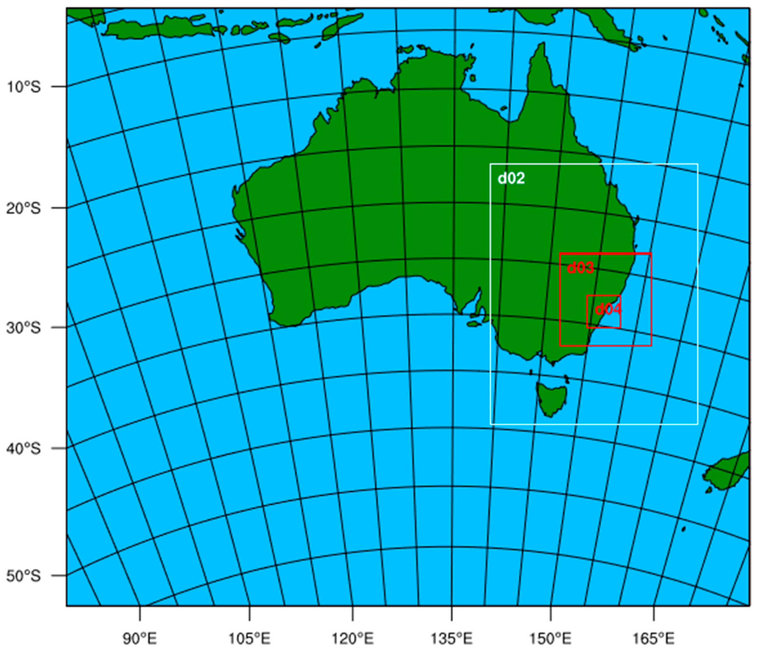
2.2. Model Configurations
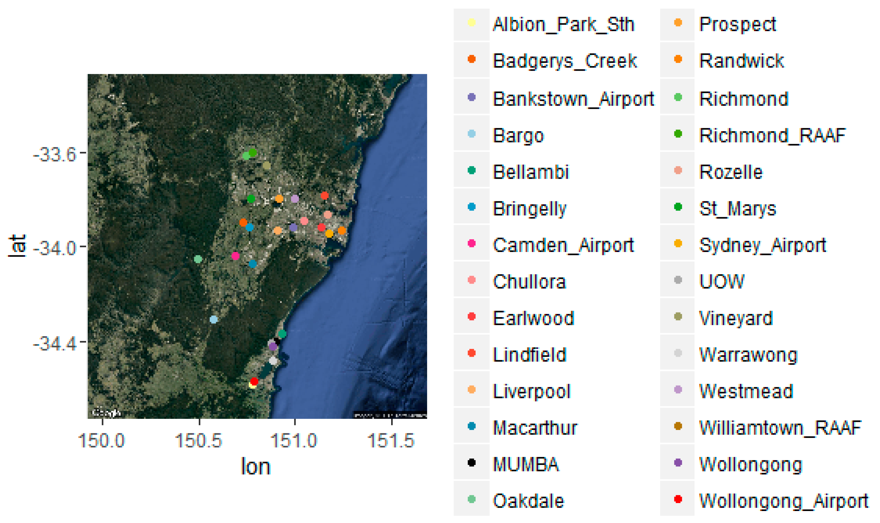
2.3. Evaluation Datasets and Protocols
3. Model Evaluation
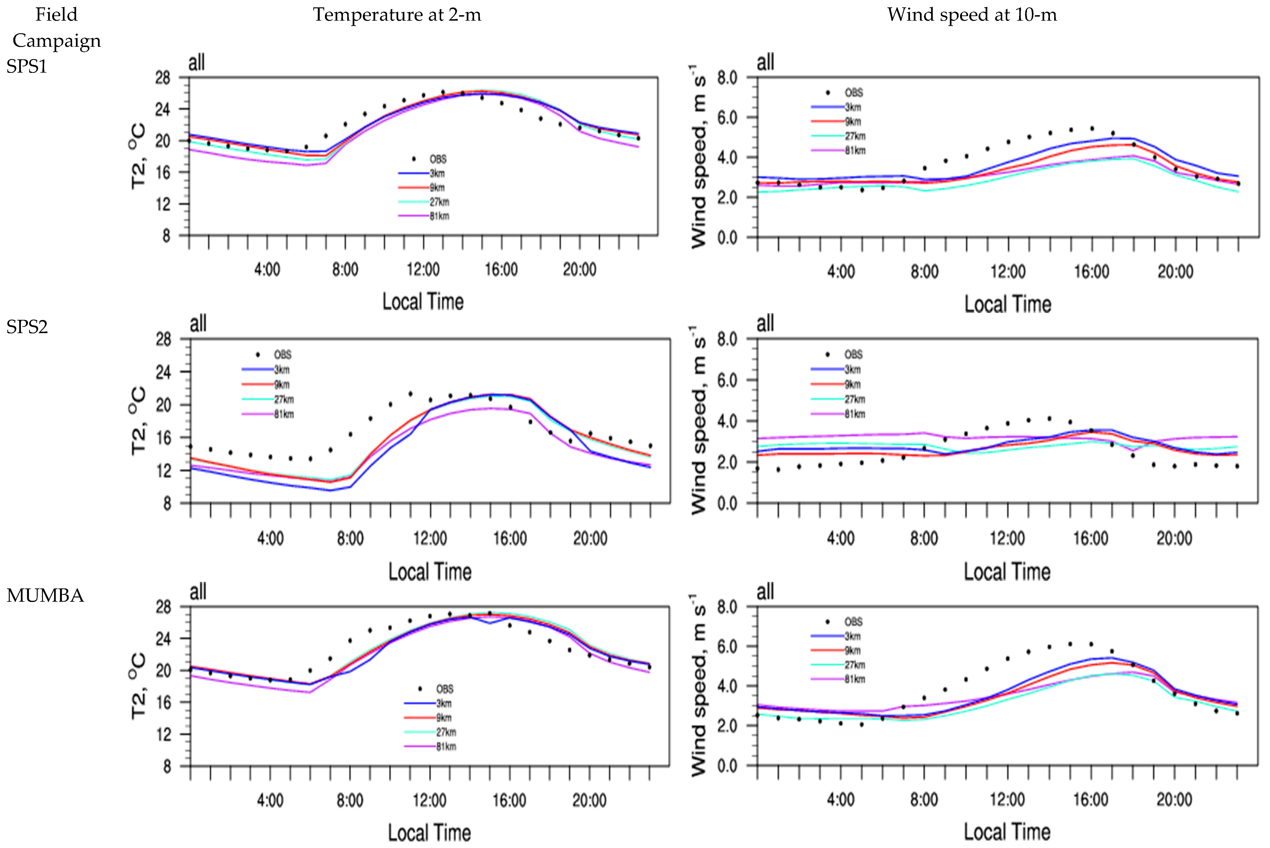
3.1. Boundary Layer Meteorological Evaluation
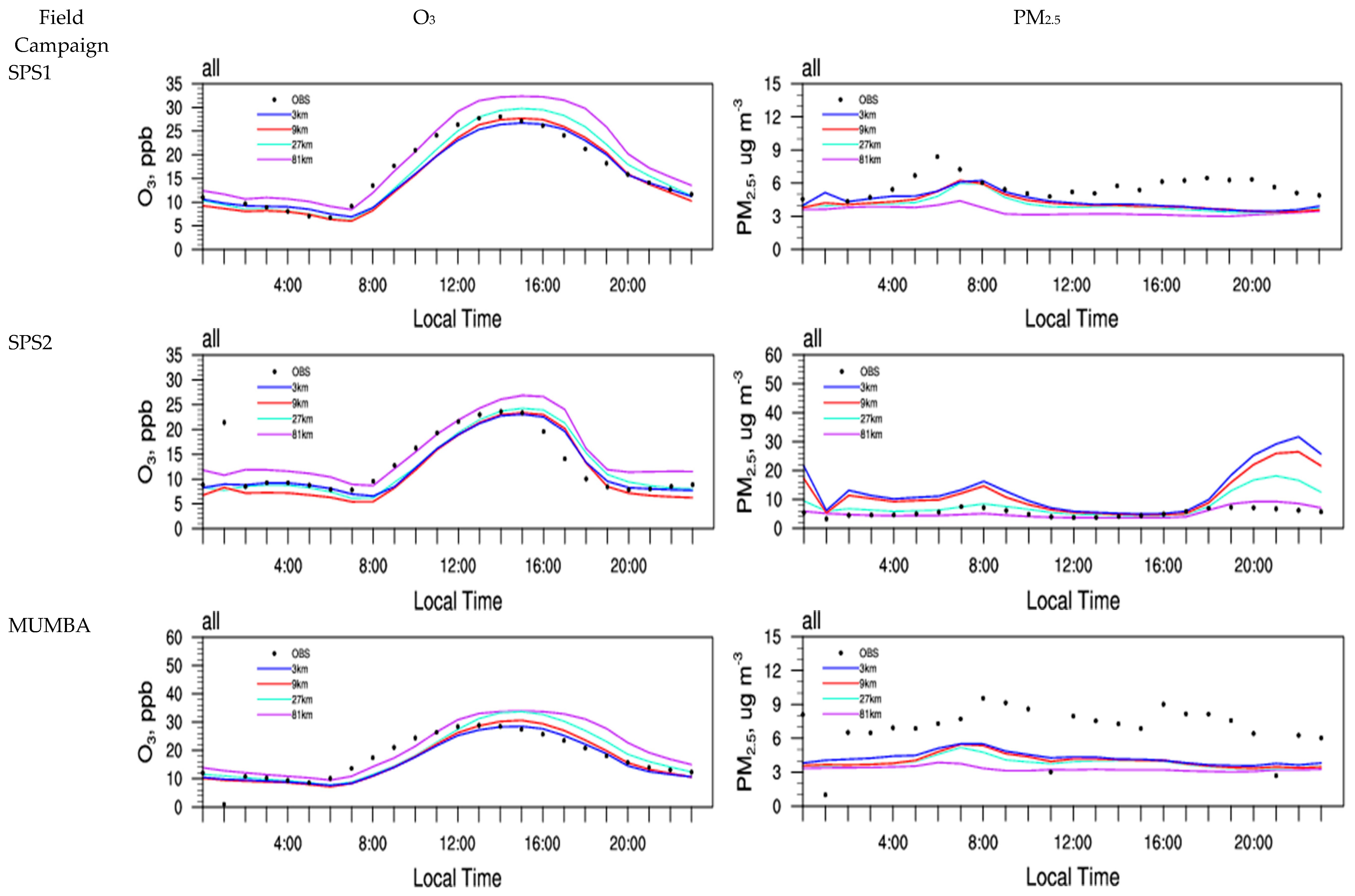
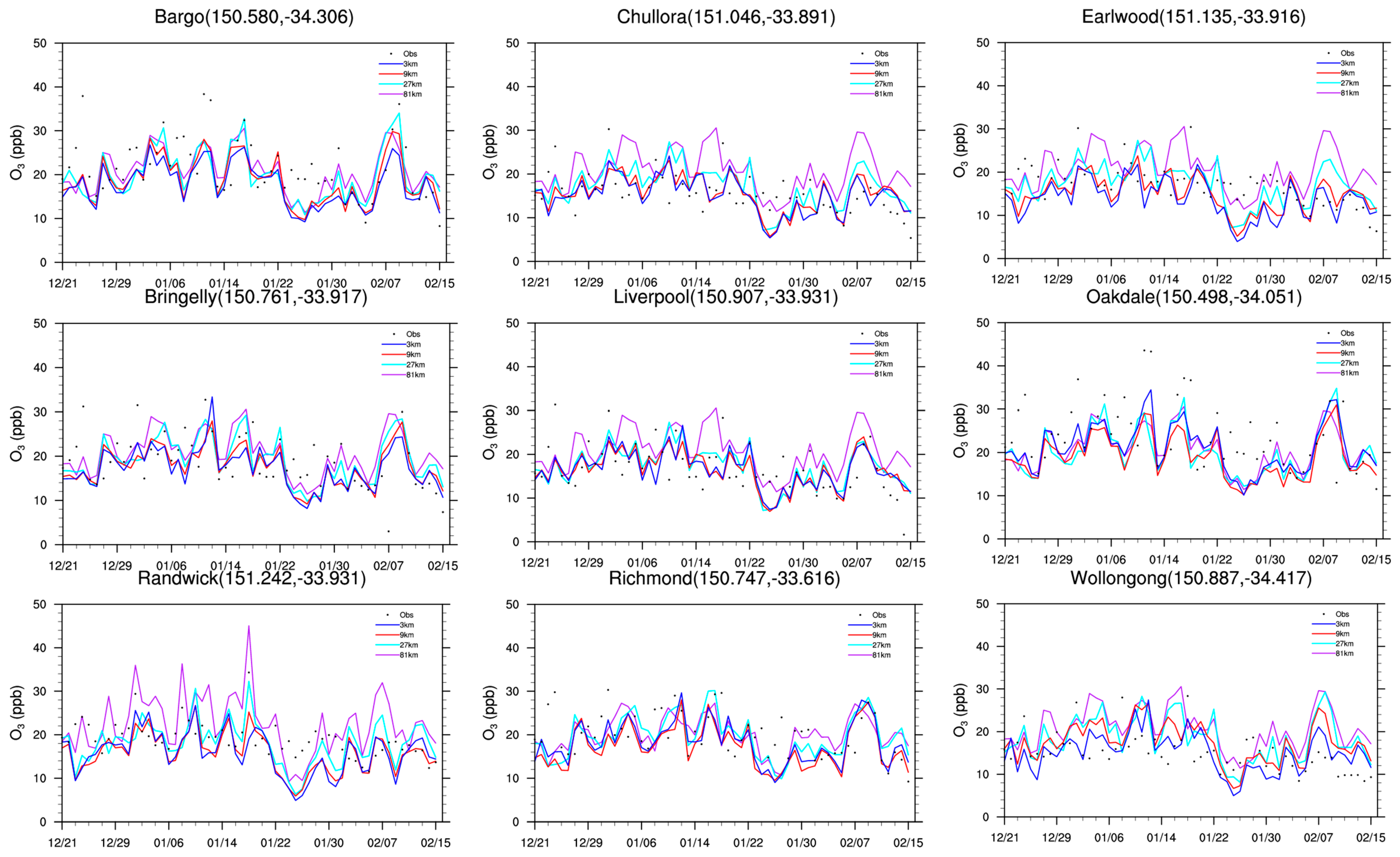
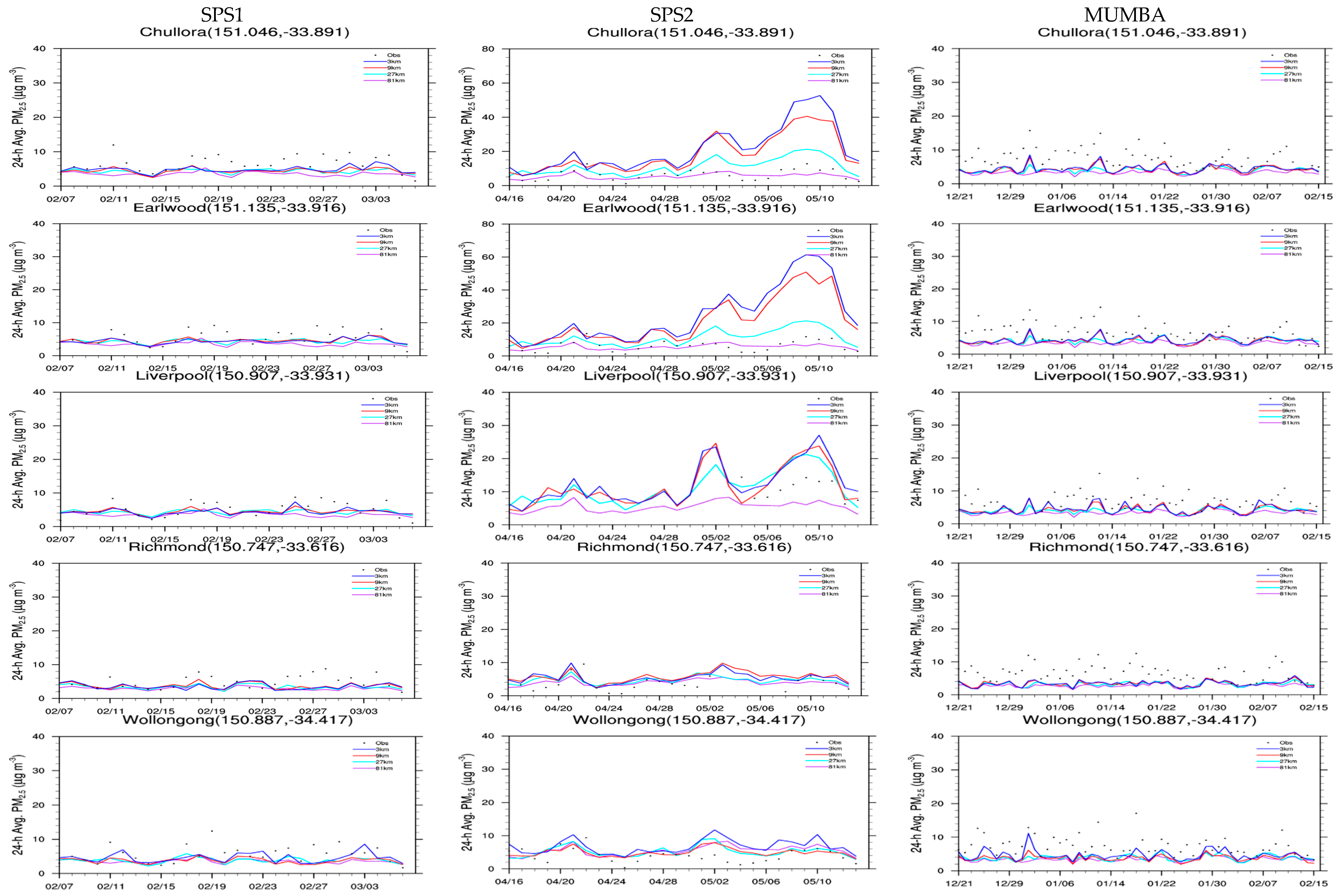
3.2. Surface Chemical Evaluation
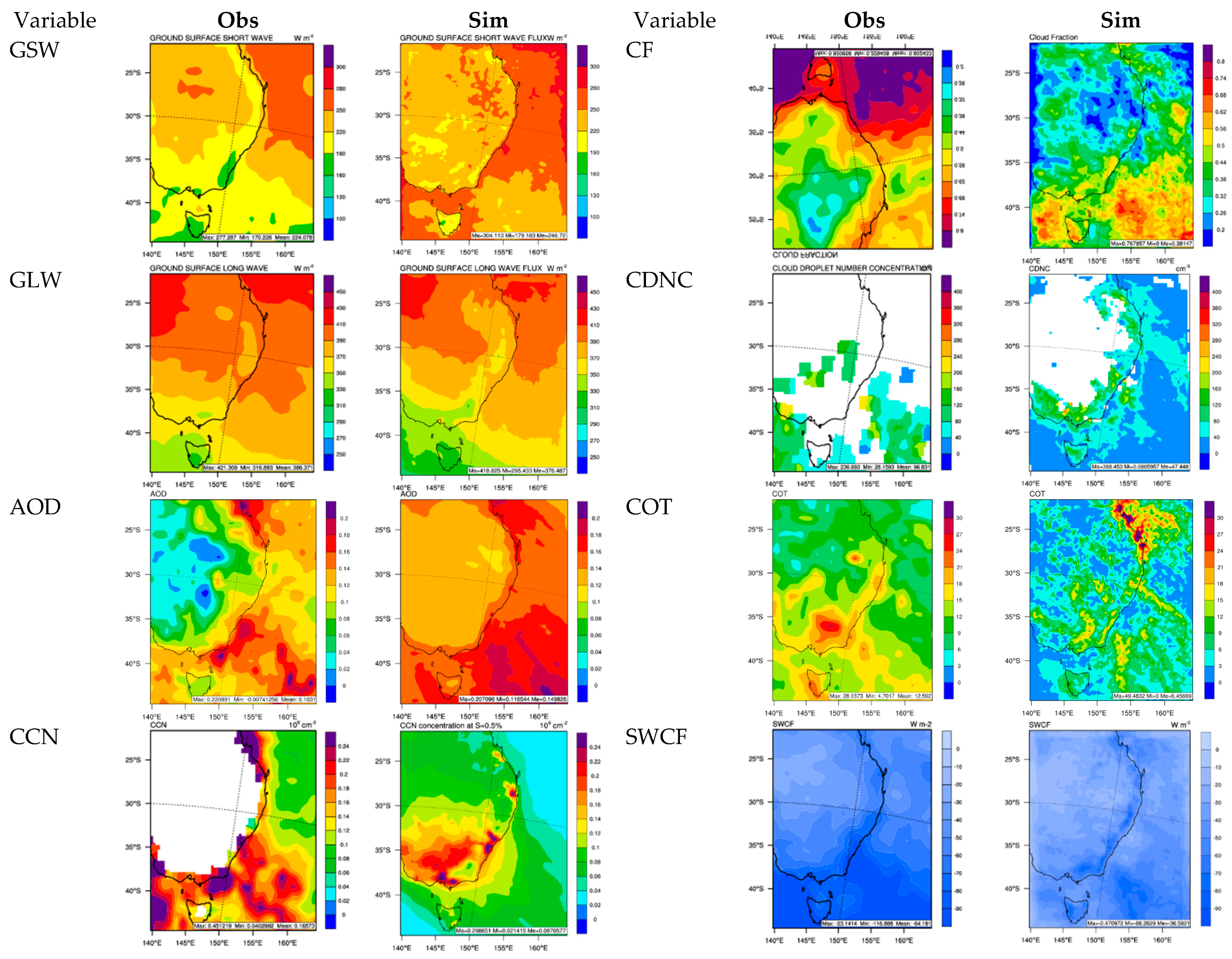
3.3. Evaluation of Radiative, Cloud, and Heat flux Variables
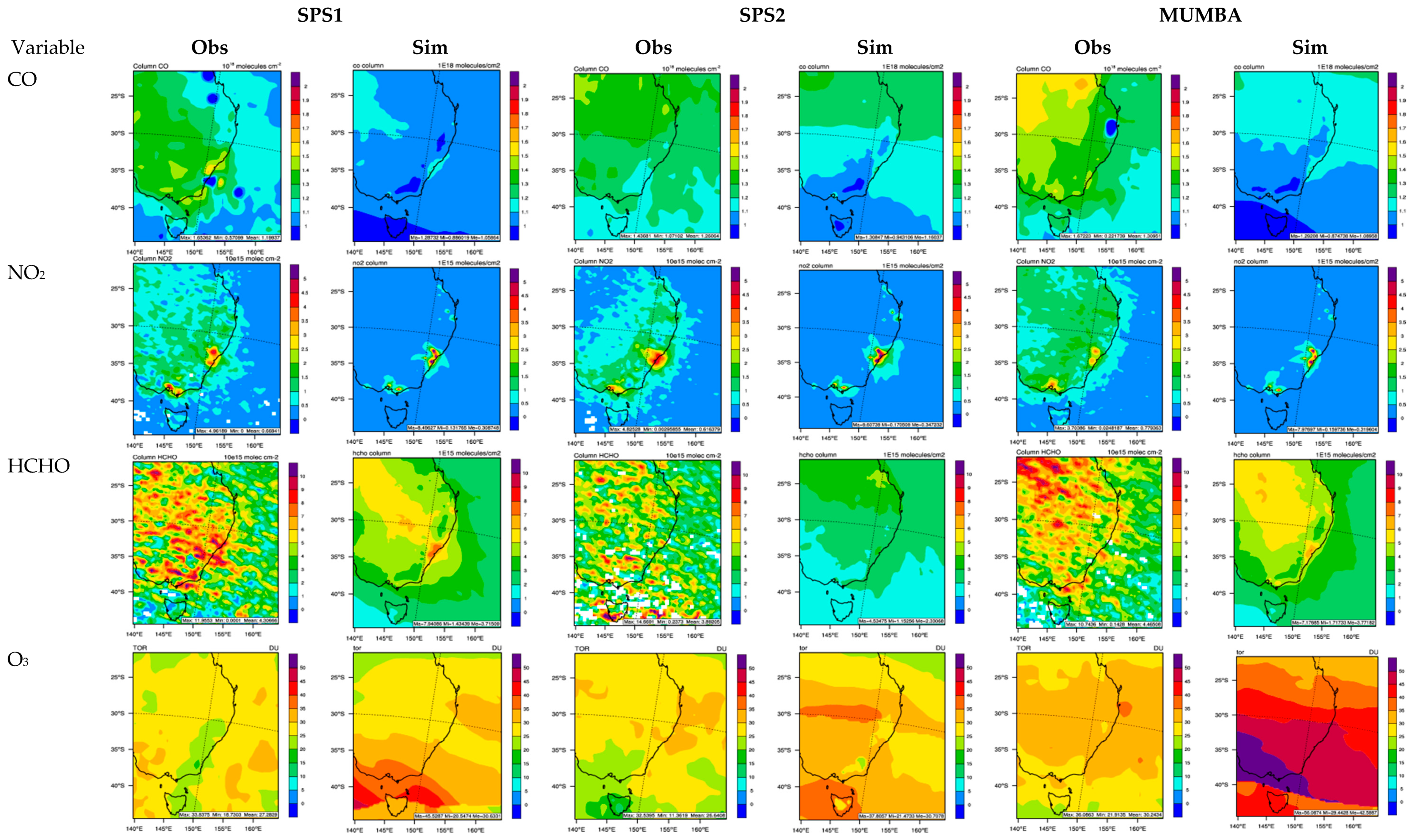
3.4. Evaluation of Column Gas Abundances
4. Conclusions
Supplementary Materials
Author Contributions
Funding
Acknowledgements
Conflicts of Interest
References
- Morgan, G.; Broome, R.; Jalaludin, B. Summary for Policy Makers of the Health Risk Assessment on Air Pollution in Australia. Available online: https://www.environment.gov.au/system/files/pages/dfe7ed5d-1eaf-4ff2-bfe7-dbb7ebaf21a9/files/summary-policy-makers-hra-air-pollution-australia.pdf (accessed on 6 April 2019).
- Keywood, M.D.; Emmerson, K.M.; Hibberd, M.F. Atmosphere: Atmosphere. In Australia State of the Environment 2016; Australian Government Department of the Environment and Energy: Canberra, Australia, 2016. Available online: https://soe.environment.gov.au/ (accessed on 6 April 2019). [CrossRef]
- Tanaka, T.Y.; Chiba, M. A numerical study of the contributions of dust source regions to the global dust budget. Glob. Planet. Chang. 2006, 52, 88–104. [Google Scholar] [CrossRef]
- Mackie, D.S.; Boyd, P.W.; McTainsh, G.H.; Tindale, N.W.; Westberry, T.K.; Hunter, K.A. Biogeochemistry of iron in Australian dust: From eolian uplift to marine uptake, Geochem. Geophys. Geosyst. 2008, 9, Q03Q08. [Google Scholar] [CrossRef]
- Gupta, P.; Christopher, S.A.; Box, M.A.; Box, G.P. Multi year satellite remote sensing of particulate matter air quality over Sydney. Aust. Int. J. Remote Sens. 2007, 28, 4483–4498. [Google Scholar] [CrossRef]
- Dirksen, R.J.; Folkert Boersma, K.; de Laat, J.; Stammes, P.; van der Werf, G.R.; Val Martin, M.; Kelder, H.M. An aerosol boomerang: Rapid around-the-world transport of smoke from the december 2006 Australian forest fires observed from space. J. Geophys. Res. Atmos. 2009, 114, D21201. [Google Scholar] [CrossRef]
- Higgenbotham, N.; Freeman, S.; Connor, L.; Albrecht, G. Environmental injustice and air pollution in coal affected communities, Hunter Valley, Australia. Health Place 2010, 16, 259–266. [Google Scholar] [CrossRef]
- Chakaraborty, J.; Green, D. Australia’s first national level quantitative environmental justice assessment of industrial air pollution. Environ. Res. Lett. 2014, 9, 044010. [Google Scholar] [CrossRef]
- Giglio, L.; Randerson, J.T.; van der Werf, G.R.; Kasibhatla, P.S.; Collatz, G.J.; Morton, D.C.; DeFries, R.S. Assessing variability and long-term trends in burned area by merging multiple satellite fire products. Biogeosciences 2010, 7, 1171–1186. [Google Scholar] [CrossRef]
- Paton-Walsh, C.; Emmons, L.K.; Wilson, S.R. Estimated total emissions of trace gases from the canberra wildfires of 2003: A new method using satellite measurements of aerosol optical depth & the mozart chemical transport model. Atmos. Chem. Phys. 2010, 10, 5739–5748. [Google Scholar]
- Paton-Walsh, C.; Emmons, L.; Wiedinmyer, C. Australia’s Black Saturday fires—Comparison of techniques for estimating emissions from vegetation fires. Atmos. Environ. 2012, 60, 262–270. [Google Scholar] [CrossRef]
- Rotstayn, L.D.; Collier, M.A.; Mitchell, R.M.; Qin, Y.; Campbell, S.K.; Dravitzki, S.M. Simulated enhancement of ENSO-related rainfall variability due to Australian dust. Atmos. Chem. Phys. 2011, 11, 6575–6592. [Google Scholar] [CrossRef]
- AAQ NEPM. Draft Variation to the National Environment Protection (Ambient Air Quality) Measure: Impact Statement; Appendix D; National Environment Protection Council, Department of the Environment: Canberra, Australia, July 2014; p. 42. Available online: https://www.environment.gov.au/protection/nepc/nepms/ambient-air-quality/variation-2014/impact-statement (accessed on 6 April 2019).
- Rea, G.; Paton-Walsh, C.; Turquety, S.; Cope, M.; Griffith, D. Impact of the New South Wales fires during October 2013 on regional air quality in eastern Australia. Atmos. Environ. 2016, 131, 150–163. [Google Scholar] [CrossRef]
- Duc, H.N.; Chang, L.T.-C.; Trieu, T.; Salter, D.; Scorgie, Y. Source Contributions to Ozone Formation in the New South Wales Greater Metropolitan Region, Australia. Atmosphere 2018, 9, 443. [Google Scholar] [CrossRef]
- Utembe, S.; Rayner, P.; Silver, J.; Guerette, E.-A.; Fisher, J.A.; Emmerson, K.; Cope, M.; Paton-Walsh, C.; Griffiths, A.D.; Duc, H.; et al. Hot summers: Effect of extreme temperatures on ozone in Sydney, Australia. Atmosphere 2018, 9, 466. [Google Scholar] [CrossRef]
- Begg, S.; Vos, T.; Barker, B.; Stevenson, C.; Stanley, L.; Lopez, A.D. The Burden of Disease and Injury in Australia 2003; Cat. No. PHE 82; Australian Institute of Health and Welfare: Canberra, Australia, 2007; p. 234. Available online: http://www.aihw.gov.au/publication-detail/?id=6442467990.BoM (accessed on 6 April 2019).
- AIHW (Australian Institute of Health and Welfare). Australian Burden of Disease Study: Impact and Causes of Illness and Death in Australia 2011; AIHW: Canberra, Australia, 2016.
- SCARC (Senate Community Affairs References Committee, Parliament of Australia). Impacts on Health of Air Quality in Australia; Senate Printing Unit, Parliament House: Canberra, Australia, 2013; p. 3.
- Broome, R.A.; Fann, N.; Cristina, T.J.; Fulcher, C.; Duc, H.; Morgan, G.G. The health benefits of reducing air pollution in Sydney, Australia. Environ. Res. 2015, 143, 19–25. [Google Scholar] [CrossRef]
- Keywood, M.D.; Galbally, I.; Crumeyrolle, S.; Miljevic, B.; Boast, K.; Chambers, S.D.; Cheng, M.; Dunne, E.; Fedele, R.; Gillett, R.; et al. Sydney Particle Study—Stage-I: Executive Summary; The Centre for Australian Weather and Climate Research: Aspendale, Australia, 2012.
- Cope, M.; Keywood, M.; Emmerson, K.; Galbally, I.; Boast, K.; Chambers, S.; Cheng, M.; Crumeyrolle, S.; Dunne, E.; Fedele, R.; et al. Sydney Particle Study—Stage-II; The Centre for Australian Weather and Climate Research: Aspendale, Australia, June 2014; ISBN 978-1-4863-0359-5.
- Paton-Walsh, C.; Guerette, E.; Kubistin, D.; Humphries, R.; Wilson, S.R.; Dominick, D.; Galbally, I.; Buchholz, R.; Bhujel, M.; Chambers, S.; et al. The MUMBA campaign: Measurements of urban, marine and biogenic air. Earth Syst. Sci. Data 2017, 9, 349–362. [Google Scholar] [CrossRef]
- Paton-Walsh, C.; Guerette, E.; Emmerson, K.; Cope, M.; Kubistin, D.; Humphries, R.; Wilson, S.R.; Buchholz, R.; Jones, N.B.; Griffith, D.W.T.; et al. Urban Air Quality in a Coastal City: Wollongong during the MUMBA Campaign. Atmosphere 2018, 9, 500. [Google Scholar] [CrossRef]
- BoM: Monthly Weather Review; Bureau of Meteorology: NSW, Sydney, Australia, February 2011.
- Chambers, S.; Williams, A.G.; Zahorowski, W.; Griffiths, A.; Crawford, J. Separating remote fetch and local mixing influences on vertical radon measurements in the lower atmosphere. Tellus B 2011, 63, 843–859. [Google Scholar] [CrossRef]
- White, C.J.; Fox-Hughes, P. Seasonal climate summary southern hemisphere (summer 2012–13): Austrlia’s hottest summer on record and extreme east coast rainfall. Aust. Meteorol. Oceanogr. J. 2013, 63, 443–456. [Google Scholar] [CrossRef]
- Monk, K.; Guérette, E.A.; Utembe, S.; Silver, J.D.; Emmerson, K.; Griffiths, A.; Duc, H.; Chang, L.T.C.; Trieu, T.; Jiang, N.; et al. Evaluation of regional air quality models over Sydney, Australia: Part 1 Meteorological model comparison. Atmosphere 2019. in review. [Google Scholar]
- Cope, M.E.; Hess, G.D.; Lee, S.; Tory, K.; Azzi, M.; Carras, J.; Lilley, W.; Manins, P.C.; Nelson, P.; Ng, L.; et al. The Australian Air Quality Forecasting System. Part I: Project description and early outcomes. J. Appl. Meteorol. 2004, 43, 649–662. [Google Scholar] [CrossRef]
- Guérette, E.-A.; Monk, K.; Emmerson, K.; Utembe, S.; Zhang, Y.; Silver, J.; Duc, H.N.; Chang, L.T.-C.; Trieu, T.; Griffiths, A.; et al. Evaluation of regional air quality models over Sydney, Australia: Part 2 Model performance for surface ozone and PM2.5. Atmosphere 2019. in preparation. [Google Scholar]
- Chang, L.T.-C.; Duc, H.N.; Scorgie, Y.; Trieu, T.; Monk, K.; Jiang, N. Performance evaluation of CCAM-CTM regional airshed modelling for the New South Wales Greater Metropolitan Region. Atmosphere 2018, 9, 486. [Google Scholar] [CrossRef]
- Grell, A.G.; Peckham, S.E.; Schmitz, R.; McKeen, S.A.; Frost, G.; Skamarock, W.C.; Eder, B. Fully coupled “online” chemistry within the WRF model. Atmos. Environ. 2005, 39, 6957–6975. [Google Scholar] [CrossRef]
- Zhang, Y.; Wen, X.-Y.; Jang, C.J. Simulating Chemistry–Aerosol–Cloud–Radiation–Climate Feedbacks over the Continental U.S. using the Online-Coupled Weather Research Forecasting Model with Chemistry (WRF/Chem). Atmos. Environ. 2010, 44, 3568–3582. [Google Scholar] [CrossRef]
- Zhang, Y.; Chen, Y.; Sarwar, G.; Schere, K. Impact of gas-phase mechanisms on Weather Research Forecasting Model with Chemistry (WRF/Chem) predictions: Mechanism implementation and comparative evaluation. J. Geophys. Res. 2012, 117, D01301. [Google Scholar] [CrossRef]
- Zhang, Y.; Karamchandani, P.; Glotfelty, T.; Streets, D.G.; Grell, G.; Nenes, A.; Yu, F.; Bennartz, R. Development and initial application of the global-through-urban weather research and forecasting model with chemistry (GU-WRF/Chem). J. Geophys. Res. 2012, 117, D20206. [Google Scholar] [CrossRef]
- Zhang, Y.; Sartelet, K.; Zhu, S.; Wang, W.; Wu, S.-Y.; Zhang, X.; Wang, K.; Tran, P.; Seigneur, C. Application of WRF/Chem-MADRID and WRF/Polyphemus in Europe, Part II: Evaluation of Chemical Concentrations and Sensitivity Simulations. Atmos. Chem. Phys. 2013, 13, 6845–6875. [Google Scholar] [CrossRef]
- Zhang, Y.; Zhang, X.; Wang, L.-T.; Zhang, Q.; Duan, F.-K.; He, K.-B. Application of WRF/Chem over East Asia: Part I. Model Evaluation and Intercomparison with MM5/CMAQ. Atmos. Environ. 2016, 124 Pt B, 285–300. [Google Scholar] [CrossRef]
- He, J.; Zhang, Y.; Wang, K.; Chen, Y.; Leung, L.R.; Fan, J.-W.; Li, M.; Zheng, B.; Zhang, Q.; Duan, F.-K.; et al. Multi-Year Application of WRF-CAM5 over East Asia-Part I: Comprehensive Evaluation and Formation Regimes of O3 and PM2.5. Atmos. Environ. 2017, 165, 122–142. [Google Scholar] [CrossRef]
- Vara-Vela, V.; Andrade, M.F.; Zhang, Y.; Kumar, P.; Ynoue, R.Y.; Souto-Oliveira, C.E.; Lopes, F.J.S.; Landulfo, E. Modelling of atmospheric aerosol properties in the Sao Paulo Metropolitan Area: The impact of biomass burning contribution. J. Geophys. Res. 2018, 123, 9935–9956. [Google Scholar] [CrossRef]
- He, J.; He, R.; Zhang, Y. Impacts of Air–sea Interactions on Regional Air Quality Predictions Using a Coupled Atmosphere-Ocean Model in Southeastern U.S. Aerosol Air Qual. Res. 2018, 18, 1044–1067. [Google Scholar] [CrossRef]
- Wang, K.; Yahya, K.; Zhang, Y.; Wu, S.-Y.; Grell, G. Implementation and Initial Application of A New Chemistry-Aerosol Option in WRF/Chem for Simulation of Secondary Organic Aerosols and Aerosol Indirect Effects. Atmos. Environ. 2015, 115, 716–732. [Google Scholar] [CrossRef]
- Yahya, K.; Glotfelty, T.; Wang, K.; Zhang, Y.; Nenes, A. Modeling Regional Air Quality and Climate: Improving Organic Aerosol and Aerosol Activation Processes in WRF/Chem version 3.7.1. Geosci. Model Dev. 2017, 10, 2333–2363. [Google Scholar] [CrossRef]
- Warner, J.C.; Armstrong, B.; He, R.; Zambon, J.B. Development of a coupled ocean-atmosphere-wave-sediment transport (COWAST) modeling system. Ocean Model. 2010, 35, 230–244. [Google Scholar] [CrossRef]
- Shchepetkin, A.F.; McWilliams, J.C. The Regional Ocean Modeling System: A split-explicit, free-surface, topography following coordinates ocean model. Ocean Model. 2005, 9, 347–404. [Google Scholar] [CrossRef]
- Marchesiello, P.; McWilliams, J.C.; Shchepetkin, A. Equilibrium structure and dynamics of the California current system. J. Phys. Oceanogr. 2003, 33, 753–783. [Google Scholar] [CrossRef]
- He, R.; Wilkin, J.L. Barotropic tides on the southeast New England shelf: A view from a hybrid data assimilative modeling approach. J. Geophys. Res. 2006, 111, C08002. [Google Scholar] [CrossRef]
- He, R.; McGillicuddy, D.J., Jr.; Keafer, B.A.; Anderson, D.M. Historic 2005 toxic bloom of Alexandrium fundyense in the western Gulf of Maine: 2. Coupled biological numerical modeling. J. Geophys. Res. 2008, 113, C07040. [Google Scholar] [CrossRef]
- Clough, S.A.; Shephard, M.W.; Mlawer, J.E.; Delamere, J.S.; Iacono, M.J.; Cady-Pereira, K.; Boukabara, S.; Brown, P.D. Atmospheric radiative transfer modeling: A summary of the AER codes. J. Quant. Spectrosc. Radiat. Transf. 2005, 91, 233–244. [Google Scholar] [CrossRef]
- Hong, S.-Y.; Noh, Y.; Dudhia, J. A new vertical diffusion package with an explicit treatment of entrainment processes. Mon. Weather Rev. 2006, 134, 2318–2341. [Google Scholar] [CrossRef]
- Hong, S.-Y. A new stable boundary-layer mixing scheme and its impact on the simulated East Asian summer monsoon. Q. J. R. Meteorol. Soc. 2010, 136, 1481–1496. [Google Scholar] [CrossRef]
- Chen, F.; Dudhia, J. Coupling an advanced land-surface/hydrology model with the Penn State/NCAR MM5 modeling system. Part I: Model implementation and sensitivity. Mon. Weather Rev. 2001, 129, 569–585. [Google Scholar] [CrossRef]
- Ek, M.B.; Mitchell, K.B.; Lin, Y.; Rogers, B.; Grunmann, P.; Koren, V.; Gayno, G.; Tarpley, J.D. Implementation of NOAH land surface model advances in the National Centers for Environmental Prediction operational mesoscale Eta model. J. Geophys. Res. 2003, 108, 8851. [Google Scholar] [CrossRef]
- Morrison, H.; Thompson, G.; Tatarskii, V. Impact of cloud microphysics on the development of trailing stratiform precipitation in a simulated squall line: Comparison of one- and two-moment schemes. Mon. Weather Rev. 2009, 137, 991–1007. [Google Scholar] [CrossRef]
- Zheng, Y.; Alapaty, K.; Herwehe, J.; Del Genio, A.; Niyogi, D. Improving high-resolution weather forecasts using the Weather Research and Forecasting (WRF) model with an updated Kain–Fritsch scheme. Mon. Weather Rev. 2016, 144, 833–860. [Google Scholar] [CrossRef]
- Yarwood, G.; Rao, S.; Yocke, M.; Whitten, G.Z. Final Report—Updates to the Carbon Bond Chemical Mechanism: CB05; Rep. RT-04-00675; Yocke and Co.: Novato, CA, USA, 2015; 246p. [Google Scholar]
- Sarwar, G.; Luecken, D.; Yarwood, G. Chapter 2.9: Developing and implementing an updated chlorine chemistry into the community multiscale air quality model. Dev. Environ. Sci. 2007, 6, 168–176. [Google Scholar] [CrossRef]
- Ahmadov, R.; McKeen, S.A.; Robinson, A.L.; Bareini, R.; Middlebrook, A.M.; De Gouw, J.A.; Meagher, J.; Hsie, E.-Y.; Edgerton, E.; Shaw, S.; et al. A volatility basis set model for summertime secondary organic aerosols over the eastern United States in 2006. J. Geophys. Res. 2012, 117. [Google Scholar] [CrossRef]
- Sarwar, G.; Fahey, K.; Napelenok, S.; Roselle, S.; Mathur, R. Examining the impact of CMAQ model updates on aerosol sulfate predictions. In Proceedings of the 10th Annual CMAS Models-3 User’s Conference, Chapel Hill, NC, USA, 24–26 October 2011. [Google Scholar]
- Abdul-Razzak, H.; Ghan, S. A parameterization of aerosol activation: 2. Multiple aerosol types. J. Geophys. Res. 2000, 105, 6837–6844. [Google Scholar] [CrossRef]
- Abdul-Razzak, H.; Ghan, S.J. A parameterization of aerosol activation, 3, Sectional representation. J. Geophys. Res. 2002, 107, 4026. [Google Scholar] [CrossRef]
- Chapman, E.G.; Gustafson, W.I., Jr.; Easter, R.C.; Barnard, J.C.; Ghan, S.J.; Pekour, M.S.; Fast, J.D. Coupling aerosol-cloud-radiative processes in the WRF-Chem model: Investigating the radiative impact of elevated point sources. Atmos. Chem. Phys. 2009, 9, 945–964. [Google Scholar] [CrossRef]
- Ghan, S.J.; Leung, L.R.; Easter, R.C.; Abdul-Razzak, H. Prediction of cloud droplet number in a general circulation model. J. Geophys. Res. 1997, 112, 21777–21794. [Google Scholar] [CrossRef]
- Liu, Y.; Daum, P.H.; McGraw, R.L. Size truncation effect, threshold behavior, and a new type of autoconversion parameterization. Geophys. Res. Lett. 2005, 32, L11811. [Google Scholar] [CrossRef]
- Chen, F.; Miao, S.; Tewari, M.; Bao, J.-W.; Kusaka, H. A numerical study of interactions between surface forcing and sea breeze circulations and their effects on stagnation in the greater Houston area. J. Geophys. Res. 2011, 116, D12105. [Google Scholar] [CrossRef]
- Seo, H.; Subramanian, A.C.; Miller, A.J.; Cavanaugh, N.R. Coupled Impacts of the Diurnal Cycle of Sea Surface Temperature on the Madden–Julian Oscillation. J. Clim. 2014, 27, 8422–8443. [Google Scholar] [CrossRef]
- Yahya, K.; Wang, K.; Gudoshava, M.; Glotfelty, T.; Zhang, Y. Application of WRF/Chem over North America under the AQMEII Phase 2. Part I. Comprehensive Evaluation of 2006 Simulation. Atmos. Environ. 2014, 115, 733–755. [Google Scholar] [CrossRef]
- Yahya, K.; Wang, K.; Zhang, Y.; Kleindienst, T.E. Application of WRF/Chem over North America under the AQMEII Phase 2—Part 2: Evaluation of 2010 application and responses if air quality and meteorology–chemistry interactions to changes in emissions and meteorology from 2006 to 2010. Geosci. Model Dev. 2015, 8, 2095–2117. [Google Scholar] [CrossRef]
- Yahya, K.; Wang, K.; Campbell, P.; Chen, Y.; Glotfelty, T.; He, J.; Pirhalla, M.; Zhang, Y. Decadal Application of WRF/Chem for Regional Air Quality and Climate Modeling over the U.S. under the Representative Concentration Pathways Scenarios. Part 1: Model Evaluation and Impact of Downscaling. Atmos. Environ. 2017, 152, 562–583. [Google Scholar] [CrossRef]
- Yahya, K.; Campbell, P.; Zhang, Y. Decadal Application of WRF/Chem for Regional Air Quality and Climate Modeling over the U.S. under the Representative Concentration Pathways Scenarios. Part 2: Current vs. Future simulations. Atmos. Environ. 2017, 152, 584–604. [Google Scholar] [CrossRef]
- Thiébaux, H.J.; Rogers, E.; Wang, W.; Katz, B. A new high-resolution blended real-time global sea surface temperature analysis. Bull. Am. Meteorol. Soc. 2003, 84, 645–656. [Google Scholar] [CrossRef]
- Reynolds, R.W.; Smith, T.M.; Liu, C.; Chelton, D.B.; Casey, K.S.; Schlax, M.G. Daily high-resolution-blended analyses for sea surface temperature. J. Clim. 2007, 40, 5473–5496. [Google Scholar] [CrossRef]
- EPA. 2008 Calendar Year Air Emissions Inventory for the Greater Metropolitan Region in NSW. Available online: https://www.epa.nsw.gov.au/your-environment/air/air-emissions-inventory/airemissions-inventory-2008 (accessed on 1 March 2018).
- Guenther, A.; Kart, T.; Harley, P.; Wiedinmyer, C.; Palmer, P.I.; Geron, C. Estimates of global terrestrial isoprene emissions using MEGAN (Model of Emissions of Gases and Aerosols from Nature). Atmos. Chem. Phys. 2006, 6, 3181–3210. [Google Scholar] [CrossRef]
- Jones, S.; Creighton, G. AFWA dust emission scheme for WRF/Chem-GOCART. In Proceedings of the 2011 WRF Workshop, Boulder, CO, USA, 20–24 June 2011. [Google Scholar]
- Gong, S.; Barrie, L.A.; Blanchet, J.P. Modeling sea salt aerosols in the atmosphere: 1. Model development. J. Geophys. Res. 1997, 102, 3805–3818. [Google Scholar] [CrossRef]
- Gantt, B.; He, J.; Zhang, X.; Zhang, Y.; Nenes, A. Incorporation of advanced aerosol activation treatments into CESM/CAM5: Model evaluation and impacts on aerosol indirect effects. Atmos. Chem. Phys. 2014, 14, 7485–7497. [Google Scholar] [CrossRef]
- He, J.; Zhang, Y. Improvement and Further Development in CESM/CAM5: Gas-Phase Chemistry and Inorganic Aerosol Treatments. Atmos. Chem. Phys. 2014, 14, 9171–9200. [Google Scholar] [CrossRef]
- Glotfelty, T.; He, J.; Zhang, Y. Impact of Future Climate Policy Scenarios on Air Quality and Aerosol/Cloud Interactions using an Advanced Version of CESM/CAM5: Part I. Model Evaluation for the Current Decadal Simulations. Atmos. Environ. 2017, 152, 222–239. [Google Scholar] [CrossRef]
- Beck, H.E.; van Dijk, A.I.J.M.; Levizzani, V.; Schellekens, J.; Miralles, D.G.; Martens, B.; de Roo, A. MSWEP: 3-hourly 0.25 global gridded precipitation (1979–2015) by merging gauge, satellite, and reanalysis data. Hydrol. Earth Syst. Sci. 2017, 21, 589–615. [Google Scholar] [CrossRef]
- Bennartz, R. Global assessment of marine boundary layer cloud droplet number concentration from satellite. J. Geophys. Res. 2007, 112, D02201. [Google Scholar] [CrossRef]
- Yu, L.; Jin, X.; Weller, R.A. Multidecade Global Flux Datasets from the Objectively Analyzed Air–Sea Fluxes (OAFlux) Project: Latent and Sensible Heat Fluxes, Ocean Evaporation, and Related Surface Meteorological Variables; OAFlux Project Technical Report, OA-2008-01; Woods Hole Oceanographic Institution: Woods Hole, MA, USA, 2008; 64p, Available online: http://oaflux.whoi.edu/pdfs/OAFlux_TechReport_3rd_release.pdf (accessed on 6 April 2019).
- Emery, C.; Tai, E. Enhanced Meteorological Modeling and Performance Evaluation for Two Texas Ozone Episodes; Project Report Prepared for the Texas Natural Resource Conservation Commission; ENVIRON International Corporation: Novato, CA, USA, 2001. [Google Scholar]
- Tesche, T.W.; Tremback, C. Operational Evaluation of the MM5 Meteorological Model over the Continental United States: Protocol for Annual and Episodic Evaluation; Draft Protocol Prepared under Task Order 4TCG-68027015 for the Office of Air Quality Planning and Standards; U.S. Environmental Protection Agency: Research Triangle Park, NC, USA, 2002.
- Wu, S.-Y.; Krishnan, S.; Zhang, Y.; Aneja, V. Modeling Atmospheric Transport and Fate of Ammonia in North Carolina, Part I. Evaluation of Meteorological and Chemical Predictions. Atmos. Environ. 2008, 42, 3419–3436. [Google Scholar] [CrossRef]
- Zhang, Y.; Liu, P.; Pun, B.; Seigneur, C. A Comprehensive Performance Evaluation of MM5-CMAQ for the Summer 1999 Southern Oxidants Study Episode, Part-I. Evaluation Protocols, Databases and Meteorological Predictions. Atmos. Environ. 2006, 40, 4825–4838. [Google Scholar] [CrossRef]
- Zhang, Y.; Cheng, S.-H.; Chen, Y.-S.; Wang, W.-X. Application of MM5 in China: Model Evaluation, Seasonal Variations, and Sensitivity to Horizontal Grid Resolutions. Atmos. Environ. 2011, 45, 3454–3465. [Google Scholar] [CrossRef]
- Penrod, A.; Zhang, Y.; Wang, K.; Wu, S.-Y.; Leung, R.L. Impacts of future climate and emission changes on U.S. air quality. Atmos. Environ. 2014, 89, 533–547. [Google Scholar] [CrossRef]
- Yahya, K.; He, J.; Zhang, Y. Multiyear Applications of WRF/Chem over Continental U.S.: Model Evaluation, Variation Trend, and Impacts of Boundary Conditions. J. Geophys. Res. 2015, 120, 12748–12777. [Google Scholar] [CrossRef]
- Wang, K.; Zhang, Y.; Zhang, X.; Fan, J.-W.; Leung, L.R.; Zheng, B.; Zhang, Q.; He, K.-B. Fine-Scale Application of WRF-CAM5 during a dust storm episode over East Asia: Sensitivity to grid resolutions and aerosol activation parameterizations. Atmos. Environ. 2018, 176, 1–20. [Google Scholar] [CrossRef]
- Zhang, Y.; Liu, P.; Queen, A.; Misenis, C.; Pun, B.; Seigneur, C.; Wu, S.-Y. A Comprehensive Performance Evaluation of MM5-CMAQ for the Summer 1999 Southern Oxidants Study Episode, Part-II. Gas and Aerosol Predictions. Atmos. Environ. 2006, 40, 4839–4855. [Google Scholar] [CrossRef]
- Yu, S.; Eder, B.; Dennis, R.; Chu, S.-H.; Schwartz, S. New unbiased symmetric metrics for evaluation of air quality models. Atmos. Sci. Lett. 2006, 7, 26–34. [Google Scholar] [CrossRef]
- Zhang, Y.; Wen, X.-Y.; Wang, K.; Vijayaraghavan, K.; Jacobson, M.Z. Probing into Regional Ozone and Particulate Matter Pollution in the United States: 2. An Examination of Formation Mechanisms Through A Process Analysis Technique and Sensitivity Study. J. Geophys. Res. 2009, 114, D22305. [Google Scholar] [CrossRef]
- Hogrefe, C.; Hao, W.; Civerolo, K.; Ku, J.Y.; Sistla, G.; Gaza, R.S.; Sedefian, L.; Schere, K.; Gilliland, A.; Mathur, R. Daily simulation of ozone and fine particulates over New York State: Findings and challenges. J. Appl. Meteorol. Climatol. 2007, 46, 961–979. [Google Scholar] [CrossRef]
- Emery, C.; Jung, J.; Downey, N.; Johnson, J.; Jimenez, M.; Yarwood, G.; Morris, R. Regional and global modeling estimates of policy relevant background ozone over the United States. Atmos. Environ. 2002, 47, 206–217. [Google Scholar] [CrossRef]
- Emery, C.; Liu, Z.; Russell, A.G.; Odman, M.T.; Yarwood, G.; Kumar, N. Recommendations on statistics and benchmarks to assess photochemical model performance. J. Air Waste Manag. Assoc. 2017, 67, 582–598. [Google Scholar] [CrossRef]
- Mass, C.; Ovens, D. WRF model physics: Problems, solutions and a new paradigm for progress. In Proceedings of the 2010 WRF Users’ Workshop, Boulder, CO, USA, 15–21 June 2010. [Google Scholar]
- Zhang, H.; Chen, G.; Hu, J.; Chen, S.H.; Wiedinmyer, C.; Kleeman, M.; Ying, Q. Evaluation of a seven-year air quality simulation using the Weather Research and Forecasting (WRF)/Community Multiscale Air Quality (CMAQ) models in the eastern United States. Sci. Total Environ. 2014, 473–474, 275–285. [Google Scholar] [CrossRef]
- Storm, B.; Dudhia, J.; Basu, S.; Swift, A.; Giammanco, I. Evaluation of the weather research and forecasting model on forecasting low-level jets: Implications for wind energy. Wind Energy 2009, 12, 81–90. [Google Scholar] [CrossRef]
- Shin, H.H.; Hong, S.Y. Intercomparison of planetary boundary layer parametrizations in the WRF model for a single day from CASES-99. Bound.-Layer Meteorol. 2011, 139, 261–281. [Google Scholar] [CrossRef]
- Draxl, C.; Hahmann, A.N.; Peña, A.; Giebel, G. Evaluating winds and vertical wind shear from Weather Research and Forecasting model forecasts using seven planetary boundary layer schemes. Wind Energy 2012, 17, 39–55. [Google Scholar] [CrossRef]
- Grell, G.A.; Devenyi, D. A generalized approach to parameterizing convection combining ensemble and data assimilation techniques. Geophys. Res. Lett. 2002, 29, 34–38. [Google Scholar] [CrossRef]
- Grell, G.A.; Freitas, S.R. A scale and aerosol aware stochastic convective parameterization for weather and air quality modeling. Atmos. Chem. Phys. 2014, 14, 5233–5250. [Google Scholar] [CrossRef]
- Wang, K.; Zhang, Y.; Yahya, K. Decadal application of WRF/Chem under current and future climate/emission scenarios, Part I: Comprehensive Evaluation and Intercomparison with Results under the RCP scenarios. 2019; in preparation. [Google Scholar]
- Chambers, S.D.; Guérette, E.-A.; Monk, K.; Griffiths, A.D.; Zhang, Y.; Duc, H.; Cope, M.; Emmerson, K.M.; Chang, L.T.; Silver, J.D.; et al. Skill-Testing Chemical Transport Models across Contrasting Atmospheric Mixing States Using Radon-222. Atmosphere 2019, 10, 25. [Google Scholar] [CrossRef]


| Variables | Mean Obs | Mean Sim | R | MB | NMB, % | NME, % | |||||||||||||||
|---|---|---|---|---|---|---|---|---|---|---|---|---|---|---|---|---|---|---|---|---|---|
| d01 | d02 | d03 | d04 | d01 | d02 | d03 | d04 | d01 | d02 | d03 | d04 | d01 | d02 | d03 | d04 | d01 | d02 | d03 | d04 | ||
| Met | |||||||||||||||||||||
| T2 (°C) | 22.1 | 21.2 | 21.9 | 22.1 | 22.2 | 0.85 | 0.86 | 0.86 | 0.86 | −0.9 | −0.22 | 0.02 | 0.09 | −4.1 | −1.0 | 0.1 | 0.4 | 9.4 | 8.6 | 7.9 | 7.8 |
| SST (°C) | 23.9 | 25.3 | 24.9 | 24.4 | 24.5 | 0.3 | −0.3 | −0.5 | 0.4 | 1.4 | 1.0 | 0.5 | 0.6 | 5.9 | 4.2 | 2.3 | 2.9 | 5.9 | 4.2 | 3.1 | 2.9 |
| RH2 (%) | 70.5 | 70.0 | 68.6 | 68.8 | 69.8 | 0.70 | 0.73 | 0.76 | 0.77 | −0.53 | −1.95 | −1.71 | −0.7 | −0.7 | −2.8 | −2.4 | −1.0 | 14.2 | 13.5 | 12.4 | 11.9 |
| WS10 (m s−1) | 3.67 | 3.11 | 2.88 | 3.32 | 3.58 | 0.44 | 0.55 | 0.66 | 0.67 | −0.56 | −0.80 | −0.35 | −0.09 | −15.3 | −21.7 | −9.7 | −2.4 | 48.9 | 46.5 | 40.5 | 39.6 |
| WD10 (°) | 150.6 | 153.0 | 160.1 | 161.9 | 160.1 | 0.79 | 0.83 | 0.83 | 0.83 | 2.40 | 9.53 | 11.3 | 9.5 | 1.6 | 6.3 | 7.5 | 6.3 | 32.6 | 30.0 | 30.9 | 30.5 |
| Precip (OBS) (mm day−1) | 0.84 | 0.96 | 0.84 | 0.66 | 0.87 | 0.26 | 0.20 | 0.06 | 0.09 | 0.12 | −0.01 | −0.18 | 0.03 | 14.1 | −0.7 | −21.5 | 3.5 | 150.9 | 148.3 | 146.8 | 159.5 |
| Precip. (MSWEP) (mm day−1) | 1.18 | 0.87 | 0.82 | 0.73 | 1.02 | 0.37 | 0.21 | 0.06 | 0.08 | −0.31 | −0.36 | −0.45 | −0.16 | −26.4 | −30.5 | −38.2 | −13.4 | 103.1 | 106.6 | 112.6 | 131.5 |
| Precip (GPCP) (mm day−1) | 2.2 | 0.9 | 0.9 | 0.7 | 0.8 | 0.1 | 0.1 | 0.1 | −0.1 | −1.3 | −1.3 | −1.5 | −1.4 | −59.1 | −56.4 | −69.6 | −62.2 | 60.0 | 57.9 | 69.7 | 66.4 |
| Chem | |||||||||||||||||||||
| O3 (ppb) | 17.0 | 20.0 | 17.1 | 15.9 | 16.1 | 0.69 | 0.73 | 0.72 | 0.71 | 2.96 | 0.09 | −1.14 | −0.97 | 17.4 | 0.5 | −6.7 | −5.7 | 42.4 | 37.0 | 36.8 | 36.5 |
| CO (ppb) | 330.6 | 121.2 | 163.7 | 147.9 | 184.2 | 0.26 | 0.18 | 0.14 | 0.07 | −209.4 | −166.9 | −182.7 | −146.4 | −63.3 | −46.6 | −55.3 | −44.3 | 64.1 | 62.5 | 66.5 | 76.0 |
| NO (ppb) | 4.86 | 0.75 | 3.30 | 4.58 | 5.11 | 0.18 | 0.28 | 0.33 | 0.30 | −4.11 | −1.56 | −0.28 | 0.26 | −84.5 | −32.0 | −5.8 | 5.0 | 94.6 | 103.6 | 113.5 | 120.4 |
| NO2 (ppb) | 6.33 | 4.29 | 6.37 | 6.67 | 6.94 | 0.38 | 0.52 | 0.49 | 0.52 | −2.05 | 0.04 | 0.34 | 0.61 | −32.3 | 0.7 | 5.4 | 9.6 | 64.3 | 58.7 | 61.4 | 62.0 |
| SO2 (ppb) | 0.61 | 0.92 | 1.23 | 1.19 | 1.31 | 0.13 | 0.21 | 0.21 | 0.21 | 0.31 | 0.62 | 0.58 | 0.70 | 50.7 | 100.9 | 94.9 | 114.3 | 158.1 | 189.5 | 186.6 | 200.8 |
| PM2.5 (μg m−3) | 5.72 | 3.42 | 4.05 | 4.20 | 4.36 | 0.01 | 0.14 | 0.27 | 0.24 | −2.30 | −1.66 | −1.51 | −1.36 | −40.2 | −29.1 | −26.5 | −23.7 | 55.9 | 52.7 | 50.8 | 52.0 |
| PM10 (μg m−3) | 17.8 | 7.2 | 7.9 | 7.9 | 8.4 | 0.04 | 0.15 | 0.24 | 0.20 | −10.6 | −9.9 | −9.8 | −9.4 | −59.4 | −55.6 | −55.4 | −52.9 | 62.8 | 59.6 | 58.5 | 59.0 |
| Variables | Mean Obs | Mean Sim | R | MB | NMB, % | NME, % | |||||||||||||||
|---|---|---|---|---|---|---|---|---|---|---|---|---|---|---|---|---|---|---|---|---|---|
| d01 | d02 | d03 | d04 | d01 | d02 | d03 | d04 | d01 | d02 | d03 | d04 | d01 | d02 | d03 | d04 | d01 | d02 | d03 | d04 | ||
| Met | |||||||||||||||||||||
| T2 (°C) | 15.7 | 15.0 | 15.8 | 15.6 | 15.8 | 0.79 | 0.82 | 0.85 | 0.84 | −0.7 | −0.1 | −0.2 | 0.1 | −4.6 | 0.6 | −1.0 | 0.4 | 14.8 | 13.5 | 12.1 | 12.1 |
| SST (°C) | 22.5 | 20.8 | 22.0 | 22.1 | 22.4 | 0.4 | 0.2 | 0.5 | 0.5 | −1.7 | −0.5 | −0.4 | −0.1 | −7.5 | −2.2 | −1.9 | −0.4 | 7.5 | 2.6 | 2.3 | 2.1 |
| RH2 (%) | 75.3 | 75.8 | 70.9 | 71.2 | 70.1 | 0.74 | 0.74 | 0.77 | 0.76 | 0.5 | −4.4 | −4.1 | −5.2 | 0.6 | −5.9 | −5.5 | −6.9 | 13.8 | 14.7 | 13.7 | 14.3 |
| WS10 (m s−1) | 2.65 | 3.65 | 3.28 | 2.77 | 2.82 | 0.43 | 0.43 | 0.55 | 0.55 | 1.00 | 0.63 | 0.12 | 0.16 | 37.6 | 23.7 | 4.4 | 6.1 | 75.7 | 70.5 | 58.3 | 57.7 |
| WD10 (°) | 189.3 | 187.8 | 192.0 | 193.5 | 191.3 | 0.85 | 0.88 | 0.88 | 0.88 | −1.6 | 2.6 | 4.2 | 1.9 | −0.8 | 1.4 | 2.2 | 1.0 | 28.4 | 26.4 | 26.1 | 25.0 |
| Precip (OBS) (mm day−1) | 4.41 | 3.25 | 3.87 | 3.08 | 3.03 | 0.73 | 0.72 | 0.90 | 0.82 | −1.16 | −0.53 | −1.33 | −1.38 | −26.3 | −12.1 | −30.2 | −31.3 | 74.4 | 71.5 | 46.7 | 56.6 |
| Precip. (MSWEP) (mm day−1) | 4.54 | 3.25 | 3.87 | 3.08 | 3.03 | 0.79 | 0.81 | 0.94 | 0.84 | −1.29 | −0.67 | −1.47 | −1.52 | −28.5 | −14.8 | −32.3 | −33.4 | 67.0 | 60.2 | 43.7 | 55.7 |
| Precip (GPCP) (mm day−1) | 2.3 | 2.5 | 2.8 | 2.3 | 2.2 | 0.8 | 0.7 | 0.5 | 0.4 | 0.2 | 0.5 | 0.0 | −0.1 | 10.6 | 23.5 | 0.3 | −6.6 | 25.9 | 42.6 | 48.7 | 56.8 |
| Chem | |||||||||||||||||||||
| O3 (ppb) | 12.9 | 15.6 | 12.9 | 11.6 | 12.5 | 0.52 | 0.59 | 0.62 | 0.60 | 2.65 | −0.02 | −1.26 | −0.44 | 20.5 | −0.2 | −9.8 | −3.4 | 56.5 | 49.8 | 48.9 | 49.4 |
| CO (ppb) | 379.6 | 155.9 | 258.0 | 263.5 | 286.6 | 0.35 | 0.38 | 0.44 | 0.31 | −223.7 | −121.6 | −116.1 | −92.9 | −58.9 | −32.0 | −30.6 | −24.5 | 61.8 | 53.8 | 55.6 | 60.9 |
| NO (ppb) | 12.6 | 1.36 | 7.0 | 13.2 | 14.3 | 0.18 | 0.40 | 0.43 | 0.41 | −11.3 | −5.63 | 0.59 | 1.65 | −89.3 | −44.6 | 4.7 | 13.0 | 94.8 | 89.8 | 105.7 | 112.9 |
| NO2 (ppb) | 9.18 | 6.48 | 9.67 | 11.0 | 11.38 | 0.40 | 0.57 | 0.58 | 0.59 | −2.71 | 0.48 | 1.84 | 2.2 | −29.5 | 5.3 | 20.1 | 24.0 | 62.9 | 56.8 | 62.8 | 64.3 |
| SO2 (ppb) | 0.61 | 1.00 | 1.44 | 1.47 | 1.59 | 0.14 | 0.21 | 0.22 | 0.21 | 0.39 | 0.82 | 0.86 | 0.98 | 63.3 | 134.8 | 141.0 | 160.5 | 159.8 | 210.0 | 216.4 | 235.2 |
| PM2.5 (μg m−3) | 5.49 | 5.31 | 8.22 | 11.8 | 13.5 | 0.27 | 0.46 | 0.43 | 0.39 | −0.18 | 2.73 | 6.3 | 8.0 | −3.4 | 49.7 | 114.8 | 145.6 | 63.7 | 87.4 | 145.2 | 171.6 |
| PM10 (μg m−3) | 14.3 | 9.3 | 11.2 | 13.0 | 14.0 | −0.01 | 0.21 | 0.28 | 0.28 | −5.0 | −3.1 | −1.33 | −0.28 | −34.9 | −21.8 | −9.3 | −1.9 | 58.0 | 55.2 | 61.0 | 65.6 |
| Variables | Mean Obs | Mean Sim | R | MB | NMB, % | NME, % | |||||||||||||||
|---|---|---|---|---|---|---|---|---|---|---|---|---|---|---|---|---|---|---|---|---|---|
| d01 | d02 | d03 | d04 | d01 | d02 | d03 | d04 | d01 | d02 | d03 | d04 | d01 | d02 | d03 | d04 | d01 | d02 | d03 | d04 | ||
| Met | |||||||||||||||||||||
| T2 (°C) | 22.5 | 22.0 | 22.6 | 22.4 | 22.3 | 0.83 | 0.84 | 0.87 | 0.87 | −0.5 | 0.1 | −0.05 | −0.2 | −2.2 | 0.4 | −0.2 | −0.9 | 9.5 | 8.9 | 87.9 | 7.8 |
| SST (°C) | 24.0 | 24.4 | 24.3 | 23.7 | 23.5 | 0.5 | 0.6 | 0.6 | 0.9 | 0.4 | 0.3 | −0.3 | −0.5 | 1.8 | 1.3 | −1.3 | −2.1 | 2.0 | 1.8 | 1.6 | 3.2 |
| RH2 (%) | 70.7 | 71.2 | 69.7 | 70.2 | 70.4 | 0.78 | 0.78 | 0.82 | 0.82 | 0.4 | −1.0 | −0.6 | −0.4 | 0.6 | −1.5 | −0.8 | −0.5 | 12.8 | 12.6 | 11.2 | 11.1 |
| WS10 (m s−1) | 3.82 | 3.98 | 3.61 | 3.53 | 3.49 | 0.26 | 0.41 | 0.68 | 0.70 | 0.16 | −0.21 | −0.29 | −0.32 | 4.3 | −5.4 | −7.5 | −8.4 | 57.8 | 50.7 | 38.8 | 37.7 |
| WD10 (°) | 138.6 | 142.0 | 149.4 | 150.1 | 149.5 | 0.80 | 0.84 | 0.85 | 0.85 | 3.4 | 10.8 | 11.5 | 10.9 | 2.4 | 7.8 | 8.3 | 7.8 | 34.3 | 30.8 | 29.6 | 28.9 |
| Precip (OBS) (mm day−1) | 5.07 | 3.43 | 3.25 | 3.40 | 3.01 | 0.86 | 0.82 | 0.86 | 0.74 | −1.65 | −1.82 | −1.67 | −2.06 | −32.4 | −35.9 | −32.9 | −40.7 | 61.8 | 68.5 | 62.0 | 69.1 |
| Precip. (MSWEP) (mm day−1) | 4.98 | 3.43 | 3.25 | 3.40 | 3.01 | 0.87 | 0.84 | 0.87 | 0.75 | −1.55 | −1.73 | −1.58 | −1.97 | −31.3 | −34.7 | −31.7 | −39.5 | 54.7 | 61.2 | 56.8 | 66.0 |
| Precip (GPCP) (mm day−1) | 5.5 | 3.2 | 3.5 | 3.2 | 2.7 | 0.7 | 0.3 | 0.5 | 0.3 | −2.3 | −2.0 | −2.3 | −2.8 | −42.2 | −36.8 | −41.9 | −50.7 | 42.2 | 36.8 | 41.9 | 51.5 |
| Chem | |||||||||||||||||||||
| O3 (ppb) | 18.3 | 21.2 | 18.8 | 17.0 | 16.4 | 0.59 | 0.63 | 0.67 | 0.68 | 2.96 | 0.52 | −1.26 | −1.84 | 16.2 | 2.8 | −6.9 | −10.1 | 46.4 | 41.8 | 38.4 | 37.5 |
| CO (ppb) | 249.4 | 112.5 | 146.6 | 139.8 | 185.7 | 0.15 | −0.02 | 0.02 | −0.01 | −136.9 | −102.8 | −109.6 | −63.7 | −54.9 | −41.2 | −43.9 | −25.5 | 62.1 | 71.3 | 72.5 | 85.4 |
| NO (ppb) | 2.66 | 0.60 | 2.18 | 3.15 | 4.07 | 0.11 | 0.28 | 0.32 | 0.28 | −2.06 | −0.48 | 0.49 | 1.41 | −77.3 | −18.1 | 18.3 | 53.2 | 97.8 | 113.1 | 131.3 | 155.4 |
| NO2 (ppb) | 4.76 | 3.32 | 5.05 | 5.65 | 6.22 | 0.42 | 0.54 | 0.53 | 0.55 | −1.44 | 0.29 | 0.90 | 1.46 | −30.2 | 6.2 | 18.8 | 30.7 | 63.2 | 62.6 | 67.5 | 71.8 |
| SO2 (ppb) | 0.61 | 0.82 | 1.12 | 1.22 | 1.53 | 0.20 | 0.26 | 0.30 | 0.30 | 0.21 | 0.51 | 0.61 | 0.92 | 33.8 | 83.5 | 98.8 | 149.6 | 145.3 | 176.2 | 183.3 | 223.0 |
| PM2.5 (μg m−3) | 7.5 | 3.3 | 3.86 | 4.0 | 4.24 | −0.04 | 0.11 | 0.24 | 0.22 | −4.2 | −3.65 | −3.51 | −3.27 | −56.4 | −48.6 | −46.7 | −43.6 | 62.8 | 58.2 | 56.6 | 55.8 |
| PM10 (μg m−3) | 20.5 | 8.3 | 9.0 | 8.9 | 9.5 | 0.06 | 0.19 | 0.26 | 0.24 | −12.2 | −11.5 | −11.6 | −10.9 | −59.4 | −56.3 | −56.4 | −53.4 | 63.6 | 60.0 | 59.4 | 58.6 |
| Satellite Variables | Network | Mean Obs | Mean Sim | R | MB | NMB, % | NME, % | |||||||||||||||
|---|---|---|---|---|---|---|---|---|---|---|---|---|---|---|---|---|---|---|---|---|---|---|
| d01 | d02 | d03 | d04 | d01 | d02 | d03 | d04 | d01 | d02 | d03 | d04 | d01 | d02 | d03 | d04 | d01 | d02 | d03 | d04 | |||
| LHF (W m−2) | OAFlux | 96.0 | 143.5 | 132.8 | 118.5 | 121.2 | 0.7 | 0.4 | 0.4 | −0.6 | 47.5 | 36.8 | 22.5 | 25.2 | 49.4 | 38.2 | 23.4 | 26.2 | 49.4 | 38.3 | 26.9 | 26.2 |
| SHF (W m−2) | OAFlux | 9.6 | 16.7 | 14.0 | 12.2 | 11.1 | −0.5 | −0.2 | −0.0 | −0.3 | 7.1 | 4.3 | 2.6 | 1.5 | 74.2 | 45.2 | 27.3 | 16.0 | 75.4 | 61.3 | 61.8 | 25.1 |
| GLW (W m−2) | CERES | 390.3 | 374.8 | 375.2 | 374.5 | 373.1 | 0.9 | 0.9 | 0.8 | 0.8 | −15.5 | −15.1 | −15.8 | −17.2 | −3.9 | −3.8 | −4.0 | −4.4 | 3.9 | 3.8 | 4.0 | 4.4 |
| GSW (W m−2) | CERES | 203.2 | 253.2 | 250.1 | 253.2 | 259.8 | 0.9 | 0.9 | 0.9 | 0.8 | 50.0 | 46.9 | 50.0 | 56.6 | 24.5 | 23.0 | 24.5 | 27.8 | 24.5 | 23.0 | 24.5 | 27.8 |
| LWCF (W m−2) | CERES | 36.9 | 20.5 | 22.1 | 21.3 | 16.5 | 0.4 | 0.5 | 0.4 | 0.3 | −16.4 | −14.8 | −15.6 | −20.4 | −44.4 | −40.0 | −42.2 | −55.1 | 44.4 | 40.0 | 42.2 | 55.1 |
| SWCF (W m−2) | CERES | −84.4 | −39.3 | −44.1 | −40.4 | −33.4 | 0.2 | 0.5 | 0.5 | 0.6 | −45.0 | −40.3 | −44.0 | −51.0 | −53.4 | −47.8 | −52.1 | −60.4 | 53.4 | 47.8 | 52.1 | 60.4 |
| AOD | MODIS | 0.14 | 0.14 | 0.15 | 0.15 | 0.15 | 0.9 | 0.8 | 0.8 | 0.8 | 0.0 | 0.01 | 0.01 | 0.01 | 1.6 | 6.4 | 8.3 | 7.3 | 9.7 | 11.6 | 12.4 | 11.6 |
| COT | MODIS | 15.7 | 4.6 | 6.0 | 3.9 | 3.1 | 0.54 | 0.64 | 0.62 | 0.53 | −11.1 | −9.7 | −11.8 | −12.6 | −70.4 | −62.0 | −74.9 | −80.4 | 70.4 | 62.0 | 74.9 | 80.4 |
| CCN | MODIS | 0.2 | 0.2 | 0.2 | 0.2 | 0.2 | 0.4 | 0.4 | 0.4 | 0.3 | −0.0 | −0.0 | −0.0 | −0.0 | −22.7 | −19.4 | −17.4 | −12.7 | 26.5 | 25.0 | 28.1 | 29.9 |
| CDNC (# m−3) | MODIS | 110.5 | 59.3 | 115.1 | 103.6 | 77.9 | 0.1 | −0.0 | −0.4 | −0.4 | −51.2 | 4.6 | −6.9 | −32.6 | −46.2 | 3.5 | −6.2 | −31.2 | 58.5 | 60.5 | 70.6 | 71.4 |
| CF | MODIS | 0.6 | 0.3 | 0.4 | 0.4 | 0.3 | 0.6 | 0.5 | 0.2 | 0.3 | −0.3 | −0.2 | −0.2 | −0.3 | −46.3 | −39.4 | −40.9 | −45.6 | 46.3 | 39.4 | 40.9 | 45.6 |
| LWP | MODIS | 123.3 | 3.9 | 7.7 | 10.1 | 13.4 | 0.3 | 0.5 | 0.5 | 0.5 | −119.4 | −115.6 | −113.2 | −109.9 | −96.8 | −93.7 | −91.7 | −89.1 | 96.8 | 93.7 | 91.7 | 89.1 |
| PWV | MODIS | 3.8 | 3.3 | 3.4 | 3.4 | 3.4 | 0.9 | 0.9 | 0.9 | 0.9 | −0.5 | −0.4 | −0.4 | −0.4 | −12.1 | −11.6 | −11.7 | −11.7 | 12.1 | 11.6 | 11.7 | 11.7 |
| Column CO (1018 molecules cm−2) | MOPITT | 1.4 | 1.1 | 1.1 | 1.1 | 1.1 | 0.2 | 0.2 | 0.2 | 0.2 | −0.3 | −0.3 | −0.3 | −0.3 | −22.0 | −21.8 | −21.6 | −21.4 | 22.2 | 21.9 | 21.8 | 21.6 |
| Column NO2 (1015 molecules cm−2) | GOME | 2.2 | 1.2 | 1.5 | 1.7 | 1.7 | 0.8 | 0.7 | 0.6 | 0.6 | −1.0 | −0.7 | −0.5 | −0.5 | −43.1 | −30.9 | −23.6 | −22.7 | 43.2 | 40.4 | 48.4 | 49.4 |
| Column HCHO (1015 molecules cm−2) | GOME | 7.3 | 6.1 | 5.8 | 5.7 | 5.7 | −0.3 | −0.2 | −0.2 | −0.2 | −1.2 | −1.5 | −1.6 | −1.6 | −16.4 | −20.5 | −22.6 | −21.7 | 24.4 | 27.2 | 28.2 | 27.6 |
| TOR (DU) | OMI | 24.5 | 31.1 | 30.7 | 30.4 | 30.2 | −0.1 | −0.2 | −0.2 | −0.2 | 6.6 | 6.2 | 5.9 | 5.7 | 26.9 | 25.2 | 23.9 | 23.1 | 26.9 | 25.2 | 23.9 | 23.1 |
| Satellite Variables | Network | Mean Obs | Mean Sim | R | MB | NMB, % | NME, % | |||||||||||||||
|---|---|---|---|---|---|---|---|---|---|---|---|---|---|---|---|---|---|---|---|---|---|---|
| d01 | d02 | d03 | d04 | d01 | d02 | d03 | d04 | d01 | d02 | d03 | d04 | d01 | d02 | d03 | d04 | d01 | d02 | d03 | d04 | |||
| LHF (W m−2) | OAFlux | 196.4 | 157.3 | 191.5 | 190.9 | 200.1 | 0.6 | 0.7 | 0.7 | 0.8 | −39.1 | −4.9 | −5.5 | 3.6 | −19.9 | −2.4 | −2.7 | 1.8 | 21.0 | 9.4 | 10.8 | 8.2 |
| SHF (W m−2) | OAFlux | 49.3 | 27.0 | 34.6 | 36.4 | 38.0 | 0.14 | 0.30 | 0.07 | 0.44 | −22.3 | −14.7 | −12.9 | −11.3 | −45.3 | −29.9 | −26.2 | −22.9 | 45.4 | 31.3 | 28.7 | 24.9 |
| GLW (W m−2) | CERES | 331.2 | 323.9 | 324.8 | 323.9 | 322.0 | 0.9 | 0.9 | 0.9 | 0.9 | −7.3 | −6.4 | −7.3 | −9.1 | −2.2 | −1.9 | −2.2 | −2.7 | 2.2 | 1.9 | 2.2 | 2.7 |
| GSW (W m−2) | CERES | 128.0 | 134.7 | 136.1 | 138.9 | 144.3 | 0.7 | 0.7 | 0.7 | 0.6 | 6.7 | 8.1 | 10.9 | 16.3 | 5.2 | 6.2 | 8.5 | 12.7 | 5.2 | 6.3 | 8.5 | 12.7 |
| LWCF (W m−2) | CERES | 24.1 | 19.5 | 21.8 | 20.4 | 15.8 | 0.9 | 0.9 | 0.9 | 0.8 | −4.6 | −2.3 | −3.7 | −8.3 | −19.0 | −9.8 | −15.2 | −34.5 | 19.1 | 10.1 | 15.5 | 34.5 |
| SWCF (W m−2) | CERES | −34.2 | −32.3 | −32.8 | −29.6 | −23.6 | 0.8 | 0.9 | 0.8 | 0.8 | −1.9 | −1.4 | −4.6 | −10.6 | −5.6 | −4.1 | −13.4 | −31.1 | 11.1 | 8.5 | 14.1 | 31.1 |
| AOD | MODIS | 0.08 | 0.14 | 0.14 | 0.14 | 0.14 | 0.8 | 0.9 | 0.9 | 0.9 | 0.06 | 0.06 | 0.06 | 0.06 | 73.6 | 76.6 | 73.4 | 71.0 | 73.6 | 76.6 | 73.4 | 71.0 |
| COT | MODIS | 14.4 | 11.7 | 11.7 | 8.0 | 5.6 | 0.5 | 0.6 | 0.5 | 0.4 | −2.7 | −2.7 | −6.4 | −8.8 | −18.7 | −19.0 | −44.5 | −61.2 | 29.3 | 36.6 | 46.7 | 64.2 |
| CCN | MODIS | 0.2 | 0.1 | 0.1 | 0.1 | 0.2 | 0.7 | 0.5 | 0.5 | 0.4 | −0.1 | −0.1 | −0.1 | −0.0 | −28.2 | −27.8 | −27.5 | −24.1 | 28.2 | 27.8 | 27.9 | 27.0 |
| CDNC (# m−3) | MODIS | - | - | - | - | - | - | - | - | - | - | - | - | - | - | - | - | - | - | - | - | - |
| CF | MODIS | 0.5 | 0.4 | 0.4 | 0.4 | 0.3 | 0.8 | 0.8 | 0.7 | 0.7 | −0.1 | −0.1 | −0.1 | −0.2 | −26.4 | −26.8 | −25.9 | −32.2 | 26.4 | 26.8 | 25.9 | 32.2 |
| LWP | MODIS | 143.0 | 7.0 | 7.4 | 8.2 | 9.1 | 0.1 | 0.3 | 0.5 | 0.4 | −136.0 | −135.6 | −134.8 | −133.9 | −95.1 | −94.7 | −94.2 | −93.6 | 95.0 | 94.7 | 94.2 | 93.6 |
| PWV | MODIS | 1.7 | 2.0 | 2.0 | 2.0 | 2.0 | 0.9 | 0.9 | 0.9 | 0.9 | 0.3 | 0.3 | 0.3 | 0.3 | 21.1 | 21.3 | 21.0 | 21.0 | 21.1 | 21.3 | 21.0 | 21.0 |
| Column CO (1018 molecules cm−2) | MOPITT | 1.2 | 1.1 | 1.1 | 1.1 | 1.1 | 0.7 | 0.5 | 0.5 | 0.4 | −0.1 | −0.1 | −0.1 | −0.1 | −7.3 | −7.1 | −7.0 | −6.8 | 7.3 | 7.2 | 7.4 | 7.3 |
| Column NO2 (1015 molecules cm−2) | GOME | 2.7 | 1.7 | 2.0 | 2.1 | 2.2 | 0.8 | 0.7 | 0.7 | 0.6 | −1.0 | −0.7 | −0.6 | −0.5 | −35.2 | −25.4 | −21.5 | −19.4 | 36.6 | 35.9 | 41.7 | 40.7 |
| Column HCHO (1015 molecules cm−2) | GOME | 3.6 | 2.7 | 2.6 | 2.6 | 2.7 | 0.2 | 0.2 | 0.2 | 0.2 | −0.9 | −1.0 | −1.0 | −0.9 | −25.0 | −26.6 | −27.4 | −25.6 | 33.0 | 33.9 | 34.4 | 33.2 |
| TOR (DU) | OMI | 28.8 | 30.3 | 30.3 | 30.1 | 30.1 | −0.8 | −0.2 | −0.4 | −0.7 | 1.5 | 1.5 | 1.3 | 1.3 | 5.2 | 5.0 | 4.4 | 4.3 | 6.1 | 5.5 | 5.2 | 5.5 |
| Satellite Variables | Network | Mean Obs | Mean Sim | R | MB | NMB, % | NME, % | |||||||||||||||
|---|---|---|---|---|---|---|---|---|---|---|---|---|---|---|---|---|---|---|---|---|---|---|
| d01 | d02 | d03 | d04 | d01 | d02 | d03 | d04 | d01 | d02 | d03 | d04 | d01 | d02 | d03 | d04 | d01 | d02 | d03 | d04 | |||
| LHF (W m−2) | OAFlux | 143.4 | 155.2 | 151.1 | 133.6 | 129.2 | 0.8 | 0.7 | 0.8 | 0.9 | 11.8 | 7.7 | −9.8 | −14.2 | 8.1 | 5.3 | −6.8 | −9.9 | 15.1 | 14.0 | 14.2 | 12.1 |
| SHF (W m−2) | OAFlux | 18.9 | 20.3 | 17.3 | 15.3 | 12.2 | −0.7 | −0.3 | −0.1 | 0.9 | 1.4 | −1.6 | −3.6 | −6.7 | 7.3 | −8.4 | −19.0 | −35.5 | 57.0 | 46.4 | 42.4 | 38.2 |
| GLW (W m−2) | CERES | 378.2 | 363.2 | 365.2 | 364.1 | 362.5 | 0.9 | 0.9 | 0.8 | 0.8 | −15.0 | −13.0 | −14.1 | −15.7 | −3.9 | −3.4 | −3.7 | −4.1 | 3.9 | 3.4 | 3.7 | 4.1 |
| GSW (W m−2) | CERES | 226.1 | 277.7 | 275.3 | 277.7 | 283.4 | 0.8 | 0.8 | 0.8 | 0.7 | 51.6 | 49.2 | 51.6 | 57.3 | 22.8 | 21.7 | 22.8 | 25.3 | 22.8 | 21.7 | 22.8 | 25.3 |
| LWCF (W m−2) | CERES | 29.6 | 10.9 | 11.5 | 10.4 | 9.2 | 0.5 | 0.2 | 0.2 | 0.5 | −18.7 | −18.1 | −19.2 | −20.4 | −63.0 | −61.2 | −64.6 | −68.8 | 63.0 | 61.2 | 64.6 | 68.8 |
| SWCF (W m−2) | CERES | −78.7 | −39.2 | −43.5 | −41.0 | −35.4 | 0.2 | 0.2 | 0.2 | 0.4 | −39.5 | −35.2 | −37.7 | −43.3 | −50.1 | −44.7 | −47.9 | −55.0 | 50.1 | 44.7 | 47.9 | 55.0 |
| AOD | MODIS | 0.12 | 0.15 | 0.16 | 0.17 | 0.16 | 0.97 | 0.95 | 0.95 | 0.96 | 0.03 | 0.04 | 0.05 | 0.04 | 27.2 | 32.3 | 34.5 | 33.0 | 27.2 | 32.3 | 34.5 | 33.0 |
| COT | MODIS | 17.0 | 10.7 | 10.1 | 6.9 | 4.9 | −0.3 | −0.4 | −0.1 | 0.1 | −6.4 | −6.9 | −10.2 | −12.1 | −37.4 | −40.5 | −59.7 | −71.0 | 37.8 | 42.7 | 59.7 | 71.0 |
| CCN | MODIS | 0.4 | 0.2 | 0.2 | 0.2 | 0.2 | 0.7 | 0.6 | 0.6 | 0.6 | −0.2 | −0.2 | −0.2 | −0.2 | −57.9 | −56.7 | −56.3 | −54.4 | 57.9 | 56.7 | 56.3 | 54.4 |
| CDNC (# m−3) | MODIS | - | - | - | - | - | - | - | - | - | - | - | - | - | - | - | - | - | - | - | - | - |
| CF | MODIS | 0.6 | 0.2 | 0.3 | 0.3 | 0.3 | 0.6 | 0.3 | 0.4 | 0.4 | −0.4 | −0.3 | −0.3 | −0.3 | −65.8 | −56.9 | −48.7 | −55.5 | 65.8 | 56.9 | 48.7 | 55.5 |
| LWP | MODIS | 148 | 4.2 | 7.7 | 11.6 | 13.4 | 0.6 | 0.5 | 0.6 | 0.5 | −143.8 | −140.3 | −136.4 | −134.6 | −97.1 | −94.7 | −92.1 | −90.9 | 97.1 | 94.7 | 92.1 | 90.9 |
| PWV | MODIS | 2.4 | 2.8 | 2.8 | 2.8 | 2.8 | 0.9 | 0.9 | 0.9 | 0.9 | 0.4 | 0.4 | 0.4 | 0.4 | 17.7 | 18.6 | 18.2 | 18.3 | 17.7 | 18.6 | 18.2 | 18.4 |
| Column CO (1018 molecules cm−2) | MOPITT | 1.3 | 1.1 | 1.1 | 1.1 | 1.1 | −0.3 | −0.1 | −0.1 | −0.1 | −0.2 | −0.2 | −0.2 | −0.2 | −17.4 | −17.2 | −17.2 | −17.0 | 17.4 | 17.2 | 17.2 | 17.1 |
| Column NO2 (1015 molecules cm−2) | GOME | 1.7 | 1.1 | 1.3 | 1.5 | 1.5 | 0.8 | 0.7 | 0.6 | 0.6 | −0.6 | −0.4 | −0.2 | −0.2 | −34.2 | −21.6 | −15.4 | −11.5 | 34.8 | 42.6 | 52.3 | 54.7 |
| Column HCHO (1015 molecules cm−2) | GOME | 5.2 | 5.2 | 4.9 | 4.6 | 4.7 | −0.1 | −0.1 | −0.1 | −0.1 | 0.0 | −0.3 | −0.6 | −0.5 | −0.1 | −7.1 | −11.4 | −10.0 | 24.5 | 27.4 | 26.8 | 27.2 |
| TOR (DU) | OMI | 32.9 | 46.8 | 46.4 | 46.2 | 46.0 | 0.5 | 0.2 | 0.2 | 0.3 | 13.9 | 13.5 | 13.3 | 13.1 | 42.0 | 40.6 | 40.1 | 39.4 | 42.0 | 40.6 | 40.1 | 39.4 |
© 2019 by the authors. Licensee MDPI, Basel, Switzerland. This article is an open access article distributed under the terms and conditions of the Creative Commons Attribution (CC BY) license (http://creativecommons.org/licenses/by/4.0/).
Share and Cite
Zhang, Y.; Jena, C.; Wang, K.; Paton-Walsh, C.; Guérette, É.-A.; Utembe, S.; Silver, J.D.; Keywood, M. Multiscale Applications of Two Online-Coupled Meteorology-Chemistry Models during Recent Field Campaigns in Australia, Part I: Model Description and WRF/Chem-ROMS Evaluation Using Surface and Satellite Data and Sensitivity to Spatial Grid Resolutions. Atmosphere 2019, 10, 189. https://doi.org/10.3390/atmos10040189
Zhang Y, Jena C, Wang K, Paton-Walsh C, Guérette É-A, Utembe S, Silver JD, Keywood M. Multiscale Applications of Two Online-Coupled Meteorology-Chemistry Models during Recent Field Campaigns in Australia, Part I: Model Description and WRF/Chem-ROMS Evaluation Using Surface and Satellite Data and Sensitivity to Spatial Grid Resolutions. Atmosphere. 2019; 10(4):189. https://doi.org/10.3390/atmos10040189
Chicago/Turabian StyleZhang, Yang, Chinmay Jena, Kai Wang, Clare Paton-Walsh, Élise-Andrée Guérette, Steven Utembe, Jeremy David Silver, and Melita Keywood. 2019. "Multiscale Applications of Two Online-Coupled Meteorology-Chemistry Models during Recent Field Campaigns in Australia, Part I: Model Description and WRF/Chem-ROMS Evaluation Using Surface and Satellite Data and Sensitivity to Spatial Grid Resolutions" Atmosphere 10, no. 4: 189. https://doi.org/10.3390/atmos10040189
APA StyleZhang, Y., Jena, C., Wang, K., Paton-Walsh, C., Guérette, É.-A., Utembe, S., Silver, J. D., & Keywood, M. (2019). Multiscale Applications of Two Online-Coupled Meteorology-Chemistry Models during Recent Field Campaigns in Australia, Part I: Model Description and WRF/Chem-ROMS Evaluation Using Surface and Satellite Data and Sensitivity to Spatial Grid Resolutions. Atmosphere, 10(4), 189. https://doi.org/10.3390/atmos10040189