Response of QIT-MS to Noble Gas Isotopic Ratios in a Simulated Venus Flyby

Abstract

The primary objective of the present study is to investigate the science return of future Venus atmosphere probe mission concepts using the Quadrupole Ion Trap (QIT) Mass Spectrometer (MS) Instrument (QIT-MS-I). We demonstrate the use of Monte-Carlo simulations in determining the optimal ion trapping conditions and focus the analysis on retrieving isotope ratios of noble gases in the model sample of the Venus atmosphere. Sampling takes place at a constant velocity of ~10 km/s between 112–110 km altitude and involves the use of getter pumps to remove all chemically-active species, retaining inert noble gases. The enriched sample is leaked into passively pumped vacuum chamber where it is analyzed by the QIT-MS sensor (QIT-MS-S) for 40 minutes. The simulated mass spectrum, as recorded by the QIT-MS-S, is deconvoluted using random walk algorithm to reveal relative abundances of noble gas isotopes. The required precision and accuracy of the deconvolution method is benchmarked against the a priori known model composition of the atmospheric sample.

1. Introduction

The miniaturization of mass spectrometers in support of space exploration programs is focused either on monitoring air quality on crewed space missions or sampling the composition of planetary atmospheres [1]. In the present study, we analyze the performance of the Quadrupole Ion Trap (QIT) Mass Spectrometer (MS) sensor (QIT-MS-S)when deployed in an atmospheric probe, such as Venus Emissivity, Radio Science, InSAR, Topography, and Spectroscopy (VERITAS) [2], or in consideration for the three major exploration themes set forth by the 2011 Planetary Decadal Survey Report [3]: (i) building new worlds, with the goal of understanding solar system origins; (ii) searching for future planetary habitats; and (iii) monitoring planetary processes through time.

Understanding the origins of the solar system relies on models of formation of Icy Planetesimals (IP) [4], which place constraints on the local physical and chemical conditions under which individual planetary bodies formed. The observed correlations [5] between the abundance of heavy elements (metallicity) in Sun-like stars and the presence of planets in their system suggest an initial accretion of IPs into a protosolar core. Models [6] assume a concurrent IP contribution to the growth of planets as the protosolar core reached a critical mass and caused a collapse of surrounding nebular gas. Planetary atmospheres are expected to be a mixture of nebular gas, dissolved impacting IPs, and traces of gas emitted from the protosolar core. As a consequence, the element composition of protosolar core IPs is believed to be similar to those of comets [7,8] but with distinctive depletion of nitrogen and argon [9]. Searches for clues about the conditions under which planets formed is focused on the composition of admixed deep atmospheres below the visible clouds, where volcanic activity supplies gases not affected by photo-dissociation and contributes to climate evolution. Atmosphere composition is defined through the abundances of major elements (noble gases, C, N, O, S, and P) relative to H. Common diagnostic isotope ratios include those of all noble gases [9], D/H, ¹²C/¹³C, and ¹⁵N/¹⁴N. These isotopic ratios characterize fractionation by thermal escape from accreting planetesimals. Abundances of nitrogen isotopes also serve as a test for the presence of the Solar Composition IPs (SCIPS) [4], believed to be formed at temperatures below 27 K as is required for equally efficient capture of all gases into IPs [10].

For proper determination of compositions of planetary atmospheres, multiple flybys or probes are needed to avoid local trajectory bias, as experienced by the quadrupole mass spectrometer [11] onboard the Galileo probe [12]. The Galileo probe encountered strong depletion of condensable gases, and as it descended, the mixing ratios of H₂O, NH₃, and H₂S rose. Mixing ratios reached constant values only for the NH₃ and H₂S gases because the Galileo Probe was below their condensation altitudes. However, the mixing ratio of water vapor (main oxygen reservoir) kept rising, even with the last measurement, because the condensation altitude for H₂O had not been reached [12]. Penetrating deep planetary atmospheres to measure nitrogen and oxygen abundances is even greater technical challenge for Uranus and Neptune, as depths above 1000 bars are required, but is feasible for “shallow” or "skimmer" atmospheric probes fabricated from nickel-chromium (Inconel 718) or titanium-6Al-4V alloys capable of withstanding ~100 bar pressure [13]. To avoid single trajectory dependence on meteorologically anomalous local conditions it is necessary to deploy multiple identical probes that synchronously penetrate atmosphere at different locations or execute multiple flybys using a single probe. For example, an array of CubeSat atmospheric "skimmers" designed to house QIT-MS can be dispersed at several locations in upper homosphere to determine noble gas abundances and isotope ratios. Early physical evolution of atmospheres of terrestrial planets is preserved in noble gas record due to their chemical inactivity to other elements. The relative abundances of noble gases are precisely known for Earth and Mars, but are still poorly understood on Venus [14], especially for heavy noble gases (Kr, Xe). Taking as an example the abundance of noble gases in the Venus atmosphere, any meaningful science return should provide following precisions: 20% for ³He; 10% for ⁴He; 6% for ¹³⁶Xe; 5% for ¹²⁴Xe, ¹²⁶Xe and ¹³¹Xe; 3% for all Ne isotopes, ¹²⁸Xe, and ¹³⁴Xe; and finally, 1% or better for all Ar and Kr isotopes as well as ¹²⁹Xe.

A competitive field of modern mass spectrometry offers instruments tuned to meet specific technological requirements. When catering to a subset of scientific requirements, each instrument projects its performance based on response function parameters. The QIT-MS sensor is no exception, and details of its response function are found elsewhere [15]. We have also developed a simulation program [16] capable of predicting QIT-MS sensor performance under a wide range of operational parameters. In this study, we go step further and simulate planetary atmosphere ‘skimmer’ probe equipped with the QIT-MS instrument and analyze its performance based on the models of atmospheric chemical composition and probe trajectory. Simulations are designed to mimic the probe entry into the Venus atmosphere and brief intake of atmospheric sample, followed by the sample preparation and subsequent analysis of isotopic ratios of noble gases. In this manner, we consider various aspects of measurements, not only the QIT-MS sensor response function. In this study, we also take into account the level of residual background gas expected to accumulate during the storage, launch, and cruise phase. Finally, we investigate how duration of the atmospheric sampling and the conductance of the sample intake interface affect the ability of QIT-MS to meet mission goals. In particular, we use Monte Carlo simulations to assess efficiency of time-limited atmospheric sampling at high probe velocities.

The present study aims to assist planetary scientists form informative decisions on requirements that are in compliance to the overall mission capabilities rather than just separately compare instrument capabilities. It also helps researchers and developers to gauge overall merit of the QIT-MS instrument when mission-specific conditions are accounted for, and only remaining source of uncertainty is the model of atmospheric composition. To monitor time-variable planetary atmospheric processes a complete inventory of relevant chemical species at high sampling rates is required. The QIT-MS instrument has the necessary analytical power: 50 full-range (10–150 u) mass spectra per second at high sensitivity (7.5 × 10¹¹ cps/Pa), supplemented with on-demand high resolution (4000 at 32 u and 5000 at 136 u) mode of operation [17]. These QIT-MS capabilities offer real-time altitude-resolved measurements of atmospheric chemical composition during probe descent below 60 km, including trace species detection and the ability to distinguish between most mass isobars.

The remainder of this paper is organized as follows. Section 2 describes the model of the experimental framework used to evaluate the performance of the QIT-MS instrument. Section 3 introduces computational models used throughout this paper. These are models of chemical composition of the Venus atmosphere, the simulated trajectory of the ‘skimmer’ atmospheric probe, the model of sample acquisition and handling and results that derive from these models, such are the post-processed chemical composition of the sample volume and performance of the QIT-MS sensor. Section 4 gives insights on simulated propagation of ion clouds in the QIT-MS-S resulting in time-of-flight mass spectra that are analyzed for isotopic ratios of noble gases using random walk deconvolution algorithm. Section 5 provides some final conclusions and directions for future work.

2. Model of the Mission Concept

Model of the Quadrupole Ion Trap Mass Spectrometer Instrument (QIT-MS-I) concept is given in Figure 1. The QIT-MS-I is designed as an atmospheric probe traveling at ~10 km/s below Venus’ homopause at 110–112 km altitude range. The composition of the Venus' atmosphere varies with altitude such that each species has its own scale height above homopause based on its own molecular mass $m_s$ [18]. Below homopause, all species have the same hydrostatic scale height derived from the local mean molecular mass $m_a$. The homopause is thus defined as the altitude at which the molecular diffusion $D_a$ and eddy diffusion $K_a$ coefficients are comparable. The dayside eddy diffusion coefficient $K_a$ has been reported at $1\times {10}^6{\mathrm{cm}}^2/\mathrm{s}$ for the entire upper atmosphere [19] and on the nightside it has a maximum of $1\times {10}^7{\mathrm{cm}}^2/\mathrm{s}$ and scales with the atmospheric density ${\rho }_a$ as $K_a\propto {\rho }_a^{-0.5}$ [20]. A homopause altitude level for the dominant species (CO₂) varies from 120 km to 131 km as illustrated in Figure 8 of Mahieux et al. [18]. Let us denote by ${\rho }_a^{*}$ the atmospheric CO₂ density for which the homopause altitude is at its lowest level (120 km). Then, it follows from Equstion (16.17) and Table 16.1 of Jacobson [21], that for nighttime homopause density of trace species ${\rho }_a^{*}(s)$ one can derive a scaling law ${\rho }_a^{*}(s)=0.5\times {(d_a/d_s)}^4 \times (1+m_a/m_s)\times {\rho }_a^{*}$, where $d_a$ and $d_s$ represent molecular collision diameters for self-diffusion and trace species diffusion in CO₂, respectively. The daytime homopause density of trace species, ${\rho }_a^{*}(s)$, scales as ${\rho }_a^{*}(s)={(d_a/d_s)}^2 \times {(0.5\times (1+m_a/m_s))}^{0.5}\times {\rho }_a^{*}$. In the case of homopause density for the helium (⁴He) relative to the CO₂, by using collision diameters from Table 16.1 of Jacobson [21], one obtains ${\rho }_a^{*}$(⁴He)$/{\rho }_a^{*}\approx 11$ for daytime and ${\rho }_a^{*}$(⁴He)$/{\rho }_a^{*}\approx 118$ for nighttime conditions, respectively. In the case of xenon (¹³⁶Xe) corresponding homopause density ratios are 0.5 and 0.7, respectively. In terms of hompause diurnal altitude levels, these values translate to altitude range of 121–122 km for xenon and 104–113 km for helium, respectively. From this analysis, we conclude that the sampling altitude of 110 km is 2.8 scale heights below the lowest xenon diurnal homopause altitude level, and that it is representative of well-mixed Venus’ atmosphere. However, for helium this sampling altitude is appropriate only on a dayside when the average CO₂ homopause altitude level is approximately 126 km [18].

The QIT-MS-I contains three major parts: (1) Sample Acquisition and Handling (SA&H) module, (2) Quadrupole Ion Trap Mass Spectrometer Sensor (QITSMS-S) and (3) Electronic module (EM). For simplicity of simulation we assume that the probe itself is kept isothermal at 300 K during sampling and measurement. The initial state of the QITMS-I is described in following.

The QIT-MS-S and SA&H are evacuated to the <1.33 × 10⁻⁸ Pa background pressure with puncture valve being installed. All the bakeout of the instrument including getter regeneration is achieved through the copper puncture tube installed in the QITMS-S 3D printed titanium vacuum chamber, see Figure 1b. Once the background vacuum levels within the instrument reach 1.33 × 10⁻⁸ Pa, the puncture tube is sealed and instrument can be deployed. We can routinely achieve these pressures within the instrument and maintain the cleanliness of the system for prolonged periods of time [23] by using the NEXTorr D100-5 ion/getter pump (SAES Getters S.p.A., Milan, Italy). The characteristic pumping speeds are as follows: 100 ℓ/s for H₂ and O₂, 70 ℓ/s for CO, 40 ℓ/s for N₂, 15 ℓ/s for CH₄, and 6 ℓ/s for noble gases. These values are for activated non-evaporative getters and will deteriorate across all species to 6 ℓ/s once the getter material is saturated.

2.1. SA&H Module

The S&H module has two functions: (1) intake of the Venus atmosphere through the sampling inlet, sample thermalization through collisions with the chamber walls and sample storage in the 1ℓ holding tank; (2) release of the gas from the holding tank into the vacuum chamber. The puncture valve keeps the system clean from the outside contaminants during the probe flight, and once punctured it remains open. In our simulations we ignore the puncture valve and assume that the Mindrum (double latching) M₁ microvalve [24] provides the same functionality (i.e., has zero leak rate when closed). This assumption is supported by the initial microvalve seat leak rate below 9 × 10⁻⁹ Paℓ/s for helium. Mindrum M₂ microvalve connects the holding tank to the vacuum chamber housing of the QIT-MS-S. Microvalves M₁ and M₂ are UHV compatible solenoid valves that can be opened and closed on demand in 2000 cycles at 200 °C and 50 cycles at −45 °C. The initial state of the SA&H is UHV, which is sustained by the CapaciTorr D100 miniature getter pump (100 ℓ/s for H₂ and O₂, 70 ℓ/s for CO), and is measured by the QIT-MS-S after opening the M₂ microvalve. Also note that the ion pump will also pump out SA&H assembly when the M₂ is open.

2.2. QIT-MS-S

The detailed description of the QIT-MS-S shown in Figure 1 is found elsewhere [15]. Briefly, QIT-MS-S is a Paul Trap sensor with custom designed detector and ionizer optics for better electron beam focusing and ion detection. In simple terms, the single ion trap cycle of measurement, shown in Figure 1c, consists of (a) ionization phase, during which ions of various m/q ratios are created and stored within the trapping volume for 5–10 ms, and (b) the analysis phase during which the ions are ejected from the trap and counted. The ejection of ions is precisely controlled in time by scanning the stability diagram using the linearly increasing ring electrode RF drive amplitude. The analysis phase can last from 1 ms to 100 ms depending on particular needs. The usual duty cycle of ion trap, defined as the ratio of duration of the analysis phase and the whole cycle, is more than 50%. The obvious advantage of the ion trap, in comparison to the linear quadrupole is that majority of ions created during ionization phase are detected, whereas for linear quadrupole filter, out of all created ions only ions with given m/q value can be analyzed at pre-programmed times transmission times.

QITMS-S is designed to operate under low-pressure conditions, where ion-neutral collisions as well as ion-ion interaction can be neglected [15]. Previous simulations [16] and measurements show that few collisions of ions with rest gas during analysis phase have negligible effect to peak shapes. These set the upper limit on the pressure within vacuum chamber not to exceed 2.7 × 10⁻⁴ Pa, which for xenon gives a 50% chance of ion-neutral collision every 14 ms. On the other hand, the ion-ion interaction is negligible if the number of ions being confined within the trap does not exceed 5000 during analysis phase. QIT-MS-S has well defined response as a function of both the pressure and the space charge [15] and is further supported by simulations which we use to predict the instrument response under various measurement conditions [16].

2.3. EM

Electronic module provides all voltage drives necessary for the operation of the instrument, the most important being RF amplitude scan function. Namely during the ionization phase the RF has a constant amplitude, whereas during the analysis phase it is linearly increased with time. For simulation purposes and without loss of generality, we use the high-purity signal generation with 1 ns time resolution. Nevertheless, the RF amplitude is modulated in random fashion in such a way that the RF amplitude at the end of analysis phase has 0.1% uncertainty. This uncertainty matches the experimentally observed instability in our RF generation submodule, giving rise to mass line broadening.

3. Computational Model

A computational model to emulate a physical system and make inferences about isotopic ratios of noble gases dissolved in CO₂/N₂ gas mixtures is given in Figure 2 as a flow chart. Briefly, each block in this flow chart represents a separate set of computer simulations dealing with a particular stage in atmospheric sample definition, its transfer and isotopic analysis. Numerical methods are used to design both the probe velocity and the trajectory. For simplicity, probe trajectory is divided into segments with either a constant velocity or a constant acceleration, and do not correspond to any specific mission. An additional constraint is imposed in requirement that the lowest point in the trajectory matches the desired sampling altitude.

The compositional model of Venus atmosphere at desired altitude is compiled from numerous data sources found in published literature, see The Venus Global Reference Atmospheric Model (Venus-GRAM) [25] and references therein. Gathered data are arranged in multidimensional arrays such that altitude-dependent number densities of molecular species, atmospheric density, kinematic viscosity, temperature, and pressure were cross-linked to trajectory data and retrievable as a function of flyby time.

The time-dependent physical properties of atmospheric sample serve as an input to the Sample Acquisition and Handling (SA&H) module. The SA&H module deals with sample thermalization and simulates the non-evaporable getter pump using variable sorption efficiency of chemically-active species. The output of the SA&H module is the composition of the sample volume that depends on already adsorbed chemically-active species. The sample volume is then released into the QITMS-S module. This module simulates the dynamics of gas flow into the vacuum chamber, controls the getter pump adsorbtion dynamics, provides the ion generation, ion confinement, and ion analysis and finally performs the analysis of isotopic ratios.

3.1. Probe Velocity and Sampling Altitude

Simulation flow chart in Figure 2 shows that SA&H module requires as one of the inputs the knowledge of probe trajectory. We numerically model a segment $zz(tt)$ of the probe trajectory as a shallow parabolic arc, such that the highest and lowest altitudes of this segment are at $z{z}_{\max }$ = 112 km and $z{z}_{\min }$ = 110 km, respectively. The flyby time scale $tt$ is such that at $t{t}_{\min }$ = 0 s and $t{t}_{\max }$ = 18.4 s probe is at its highest altitude $z{z}_{\max }$. Therefore, probe’s lowest altitude $z{z}_{\min }$ is reached at time $t{t}_{\mathrm{avr}}$ = ($t{t}_{\min }$ + $t{t}_{\max }$)/2 = 9.2 s while maintaining the constant velocity $vv$~10 km/s. Probe’s maximum horizontal and vertical displacements during this short flyby are $2aa$ = 200 km and $\Delta zz$ = $z{z}_{\max }$ − $z{z}_{\min }$ = 2 km, respectively. We model probe’s altitude $zz(tt)$ and horizontal displacement $xx(tt)$ by numerically solving system of equations,

$$\begin{array}{c}z(t)=z_{\min }+\Delta z·{(\frac{x(t)}{a}-1)}^2\\ v·(t-t_{\mathrm{avr}})=\frac{a}{2}\sqrt{1+{(\frac{2\Delta z}{a}·(\frac{x(t)}{a}-1))}^2}·\left(\frac{x(t)}{a}-1\right)+\frac{a^2}{4\Delta z}{\sinh }^{-1}(\frac{2\Delta z}{a}·(\frac{x(t)}{a}-1))\end{array}$$

(1)

Note that the sampling of the Venus atmosphere starts at instant $t_{\mathrm{avr}}$ and lasts for 2 s.

3.2. Compositional Model of Venus Atmosphere

As illustrated in Figure 2, second important input to the SA&H module is the composition of the Venus atmosphere. The time-dependent partial pressures of molecular species entering the QIT-MS-I are derived from the published data on the composition of Venus atmosphere and the simulated probe trajectory, see Equation (1). Note that the total pressure at the inlet of the instrument is a sum of static and dynamic pressures. The static pressure at 110 km is about 0.096 Pa. This value is derived from number densities of Kransopolsky [26,27] and mean VIRA [25] daytime (LST = 12 h) and nighttime (LST = 0 h) temperature data for 100–150 km altitudes. The dynamic pressure is about 4500 times larger than the static pressure at the 110 km altitude, which gives 437.3 Pa as suggested by the average mean VIRA [25] mass density, re-normalized atmospheric composition, and probe velocity.

In the current model, an increased temperature and density of gas sample in the bow shock are considered insufficient for thermal decomposition of CO₂ [28,29], noble gas partition [30], or charge transfer reactions [31,32] between noble gas atoms and CO₂ molecules. In general, thermal decomposition of CO₂ in the bow shock may include CO, O₂ and C produced in three reactions [28],

$$\begin{array}{ccc}{K}_1:C{O}_2\leftrightarrow CO+\frac{1}{2}{O}_2& K_2:2CO\leftrightarrow C{O}_2+C& K_3:C+O_2\leftrightarrow C{O}_2\end{array}$$

(2)

where the values of equilibrium constants K₁, K₂, and K₃ were calculated at each temperature $T$(up to 6000 K) using relation $ln{K}_i=a_{i,-1}{T}^{-1}+a_{i,0}+a_{i,+1}T+a_{i,+2}{T}^2$ and NIST-JANAF [29] free energy of formation data.

The coefficients $a_{i,-1}$ $a_{i,0}$, $a_{i,+1}$, and $a_{i,+2}$ are shown in

Table 1. The thermal coefficients corresponding to the three equilibria K₁, K₂, and K₃.

$\mathit{l}\mathit{n}{\mathit{K}}_{\mathit{i}}$	${\mathit{a}}_{\mathit{i},-1}\left[K\right]$	${\mathit{a}}_{\mathit{i},0}$	${\mathit{a}}_{\mathit{i},+1}\left[K^{-1}\right]$	${\mathit{a}}_{\mathit{i},+2}\left[K^{-2}\right]$
$ln{K}_1$	−33996.156	10.4805	−5.80673 × 10−5	−7.39975 × 10−9
$ln{K}_2$	20678.097	−21.3846	2.44549 × 10−4	9.98744 × 10−9
$ln{K}_3$	47314.216	0.423654	−1.28414 × 10−4	4.81206 × 10−9

, and when compared to

Table 2. Chemical model for the effective (static + dynamic) inlet partial pressures p_in of noble gases isotopes, as experienced by the sampling inlet at 110 km altitude and for probe velocity of ~10 km/s.

Isotope		pin [Pa]	Isotope		pin [Pa]
Ne	20	1.29 × 10−3	He	3	3.33 × 10−8
	21	3.33 × 10−6		4	2.47 × 10−4
	22	1.19 × 10−4	Xe	124	6.00 × 10−8
Ar	36	1.08 × 10−2		126	5.20 × 10−8
	38	2.11 × 10−3		128	1.07 × 10−6
	40	1.25 × 10−2		129	1.42 × 10−5
Kr	80	2.93 × 10−6		130	2.13 × 10−6
	82	5.60 × 10−6		131	1.08 × 10−5
	83	1.00 × 10−5		132	1.33 × 10−5
	84	2.13 × 10−5		134	4.80 × 10−6
	86	3.73 × 10−6		136	3.87 × 10−6

of Ref. [28], they yield no precipitation of carbon and up to 6% larger values for the mole fractions of CO and O₂ produced by dissociation of 1 mole of CO₂ along the phase boundary curves. Small difference is due to an extended temperature range (100–6000 K) and revised data on the free energy of formation [33]. Along the phase boundary curve, mole fraction of CO and O₂ are in range of few parts in 1 × 10¹³, and can be neglected as source of uncertainty for native CO and O₂ abundances. Thermal ionization of noble gases in the bow shock is also neglected as an unlikely contribution to isotope fractionation due to the cross-shock potential [34], but will be revisited in a future study.

The approximate chemical composition of the Venus atmosphere at 110 km altitude is shown in Table 2 and

Table 3. Same as in Table 2 but for CO₂, N₂, and trace species. Combined CO₂/N₂ contribution is 99.89%.

Species	pin [Pa]	Species	pin [Pa]
CO2	4.27 × 102	H2O	1.87 × 10−4
N2	9.87 ×100	OCS	1.73 × 10−8
O2	3.47 ×10−2	CO	2.93 × 10−1
SO2	7.07 ×10−7	NO	8.66 × 10−8
S2O	2.09 ×10−11	H2S	3.20 × 10−7
S2O2	2.17 ×10−10	S8	1.33 × 10−1

. The variation of all chemically-active trace species below 112 km altitude is adopted from the photo-chemical model of Krasnopolsky [26,27]. Altitude dependent isotopic abundances of noble gases are due to Hoffman et al. [35,36], Wieler [37], Fegley [38], and Donahue et al. [39] or where unavailable, except ⁷⁸Kr, substituted with terrestrial values due to De Laeter et al. [40] and Wieser et al. [41]. Decision to leave out ⁷⁸Kr comes from large uncertainties in atmospheric models containing isobars C₆H₆ and CS₂ and warrants a separate study. The unknown thermal production rates in the hypervelocity high-temperature (6 × 10⁴ K) bow shock as well as unknown gettering rates for these molecules contribute to unknown interference levels at m/q 78 which will be addressed in a future study. Here we assume that all chemically active species except noble gases will be removed from the gas sample by getter pumps. The calculated molecular isotope abundances are based on the algorithm of Hugentobler & Loliger [42] and are readily obtained for molecules of arbitrary chemical complexity.

Blending different data sources to infer relative abundances of chemical species requires their re-normalization. Namely, with every 0.5 km drop in altitude starting from 112 km down to 110 km, mixing ratios of noble gases and trace species were balanced by the binary mixture of 96.5% CO₂ and 3.5% N₂ and re-normalized to unity. Using the atmospheric temperature of 175 K, atmospheric mass density of 7.56 × 10⁻⁶ kg/m³, and corresponding mixing ratios, we compute the intake partial pressures for each chemical species as given in Table 2 and Table 3. These intake pressures will set the pV-flow through the sampling inlet of the SA&H module.

3.3. Model of Sample Acquisition and Handling

The next simulation phase in Figure 2 deals with the SA&H module. The pathway of Venus atmosphere sample through the SA&H module is illustrated in Figure 2. The pathway consists of the sampling inlet followed by the puncture valve and line to the Mindrum microvalve (M₁). After M₁, the sample first enters the thermalizer and then the holding tank, which is isolated from QIT-MS-S by M₂ microvalve. In this simulation phase, we replace with zero-length tube the sample line leading to the puncture valve, the puncture valve itself, and the line leading from the puncture valve to and including the M₁ valve. In addition, the sample pathway between M₁ and the holding tank and thermalizer are in our model simplified by a single stainless steel tube (SST) with length L = 10 cm and inner diameter d = 1 mm (of volume V_s) held at room temperature (300 K). The holding tank is made of the 304 stainless steel and has volume V_h = 1ℓ and mass of 15 g. The M₂ valve is connected via zero-length tubes to the sampling volume on one side and to the vacuum chamber on the other side. The realistic CO₂ flow rate through M₁/M₂ valves, as a function of the head pressure and the pumping speed of getter pumps, will be reported in a future study.

Prior to the sampling, the vacuum chamber remains isolated from the holding tank by the M₂ valve, whereas the holding tank is isolated from the sampling inlet by the M₁ valve. At this point, both the holding tank and the vacuum chamber contain only the residual gas, which is assumed here to be sustained at the background pressure of $p_b$ = 3.2 × 10⁻⁸ Pa. This estimate is based on the following composition of the background pressure [43]: H₂ (83.2%), H₂O (5.9%), N₂ (0.8%), CO (4.4%), CO₂ (5.7%). The exact compositions of the residual background pressure need to be measured, monitored, and corrected for as part of each static pressure measurement. Possible mitigations include coating of vacuum chamber’s interior surfaces by getter materials. Each of these molecular species (with mass m) will contribute its own partial pressure $p_{\mathrm{b}}^m$ to the total background pressure $p_b$. The vacuum of the system is maintained by CapaciTorr D100 getter pump [44] directly attached to the holding tank as well as ion pump / getter combination (NEXTorr D100-5) connected to the vacuum chamber (when M₂ is open). Estimated amount of gas (1Torr = 133.322 Pa) that getters need to adsorb during 2 years of background vacuum maintenance is α_H2 = 1.2 Torrℓ and α_CO2 = 0.08 Torrℓ, which is well below the single run getter capacity [45].

In the following we will describe the calculation leading to the sample volume composition, which is an output from the SA&H module. The atmosphere sampling begins by opening the ${\mathrm{M}}_1(t)$ valve for 2 s, see

Table 4. State logic for Mindrum micro valves.

Time t, (s)	Mode of Operation	M1(t)	M2(t)
65.9	start atmospheric survey	1	0
67.9	start CO2/N2 scrubbing	0	0
77.5	start enriched sample analysis	0	1
2478	end of sample analysis	0	1

. The duration of sampling depends on several, mutually interconnected requirements: (a) the anticipated inlet pressure at the lowest point in trajectory; (b) the model used to describe conductivity of the sampling inlet tube [46]; (c) the volume of the holding tank; (d) the maximum single run capacity of the getter pump used to remove CO₂ and N₂ from the holding tank; (e) the total pressure of all noble gas species in the sample upon its release into the vacuum chamber for analysis; and most importantly, (f) the scientific requirements on precision for noble gas isotopic ratios.

For a given inlet pressure, the flow of atmospheric sample is established through the sampling inlet tube. Dimensions of the inlet tube can be chosen in accordance to the total amount of gas that can be admitted into the holding tank without saturating the getter pump with CO₂ and N₂. Otherwise, the getter pump will saturate and pumping speeds for these dominant active species will remain at about 10% of their maximum values. The choice of the flow model is crucial in establishing the amount of gas that has been admitted into the holding tank via the sampling inlet. If inadequate model of molecular flow is used, even when M₁ remains open for sufficiently long time, the partial pressure of any noble gas isotope inside the holding tank will increase asymptotically only to the value at the sampling inlet, and no further enrichment is possible. The enrichment of the noble gases in the holding tank is achievable only if the dissolved flow model is used, such that the back flow of trace isotopes out of the holding tank is inhibited.

In the dissolved flow model, see Section 3.3.2, we assume all minor species are dissolved in binary CO₂/N₂ gas mixture, and according to Equation (3), will be carried through the sampling tube within the directional flow. As long as the partial pressure of CO₂ inside the holding tank remains lower than its inlet value, no back flow of dissolved noble gas isotopes is possible. The CO₂ pressure difference $p_{\mathrm{in}}(t)$ that is required to maintain the directional flow is sustained by the CapaciTorr D100 getter pump [44]. Depending on the amount of admitted sample, all noble gas isotopes can be enriched at various levels by adjusting the duration of sampling. For example, sampling through L = 10 cm long inlet tube for 2 s can achieve 11.6 factor of enrichment for ¹²⁸Xe inside the holding tank as compared to the inlet value, but it will require tube with diameter d = 6.5 mm and getter pump capable of adsorbing 37 Torr ℓ of mostly CO₂ and N₂. For tube with the diameter d = 4 mm the enrichment factor is 1.7 for ¹²⁸Xe compared to the inlet value and getter will be required to adsorb 5.4 Torr ℓ. If we instead use a tube with the diameter d = 3 mm then the depletion factor for ¹²⁸Xe is 0.54 compared to the inlet, whereas the getter must adsorb 1.8 Torr ℓ.

The depletion of partial pressures inside the holding tank is a consequence of a short sampling time for a given inlet tube conductance. Even with the depleted noble gas sample, as compared to its inlet composition, the dissolved flow model yields 1.77 times higher ¹²⁸Xe partial pressure in the holding tank compared to the molecular flow model. Therefore, for a given form factor of the sampling inlet, we can control the amount of admitted gas into the holding tank by adjusting the time for which M₁ valve remains open. Depending on the amount of admitted gas, the isotope content in the sample compared to the inlet, can be conveniently enriched or depleted. However, the admitted amount of sample must always be below the single-run adsorption capacity for the Capacitor getter. It is important to note that use of dissolved flow dynamics instead of molecular flow approximation is required for assessing the accuracy.

3.3.1. Micro Valve State Logic

Mindrum valves are operated according to the sequence given in Table 4. The zero time is defined as the time when atmospheric probe is at 200 km altitude. The sampling of Venus atmosphere begins at 65.9 s when the probe’s altitude is 110 km, see Equation (1).

At the beginning of the survey, see the first row in Table 4, the M₁ valve is open during 2 s admitting the sample of atmosphere into the holding tank, whereas the M₂ valve remains closed protecting the QIT-MS-S from the inlet pressure surge. After 2 s, see the second row in Table 4, both the M₁ and M₂ valves are closed for 9.6 s during which gettering of CO₂/N₂ and other chemically-active species is performed. When scrubbing is finished at $t$ = 77.5 s, the sample containing mostly noble gases is admitted into the vacuum chamber for mass spectrometry analysis by opening the M₂ valve, see the third row in Table 4. Upon the completion of the analysis, the ion pump is activated and both the vacuum chamber and the holding tank are pumped out and prepared for the next flyby sampling.

3.3.2. Computation of Dissolved pV-flow

We simulate the pV-flow $Q_{d,L}^m$ of gas particles (with molecular mass $m$) through narrow tubes of diameter d and length L using the closed form result of Fryer [47]:

$$\begin{gathered} Q_{d,L}^m(t)=d^3\sqrt{\frac{\pi k_{\mathrm{B}}T}{32m}}[\frac{\pi }{32}\frac{p_{\mathrm{in}}(t)}{2p_c}\left(1-e^{-{\sin \mathrm{h}}^{-1}(\frac{p_{\mathrm{in}}(t)}{2p_c})}\right)+ \\ \frac{\pi }{3}\frac{\frac{p_{\mathrm{in}}(t)}{2p_c}}{\frac{p_{\mathrm{in}}(t)}{2p_c}+1}+\frac{4}{3}\frac{1}{p_{\mathrm{in}}(t)/2p_c+1}]\times \frac{p_{\mathrm{in}}(t)}{L}, \end{gathered}$$

(3)

which is applicable to wide range of flow regimes, from molecular to viscous. The molecular mass $m$ and temperature T determine the value for the mean thermal component of gas velocity. The inlet pressure p_in governs the time-dependent directional component of velocity in tubular flow.

First term in Equation (3) accounts for the Poiseuille flow corrected for the proportion of molecules with mean free path larger than the tube diameter. Central term describes slip flow in which molecules that interact with tube walls are assumed to possess no average flow momentum. Last term in Equation (3) accounts for molecular diffusion near tube walls. The pressure gradient $p_{\mathrm{in}}/L$ in Equation (3) implicitly includes the difference between the inlet and the outlet partial pressures, because directional flow will stop when these two pressures are equal. Outlet pressure is always assumed to be downstream from the inlet. The inlet pressure will change with the flyby time during sample admission into the holding tank, mainly due to hypervelocity changes in the atmosphere composition in the bow shock (dependent on probe velocity) whereas the outlet pressure will change due to the active pumping of the holding tank.

Inlet pressure $p_{\mathrm{in}}(t)$ in Equation (3) is scaled by the characteristic pressure $p_c$:

$$p_c=\frac{k_{\mathrm{B}}T}{\sqrt{2}\pi d_m^{2}d}.$$

(4)

The $p_c$ is pressure at which molecular mean free path $\lambda$ ~$d_m^{-2}$ (for a given molecular mass m and temperature T) equals the tube diameter d, and is dominated by CO₂ gas. The collisional diameter $d_m$ in Equation (4) is dependent on molecular mass m, gas temperature, and gas pressure. We estimate the value for $d_m$ using the gas viscosity $\eta$ and the approximate relation $\eta \approx \rho \overline{c}\lambda /2$ [47], where $\rho$ and $\overline{c}$ are mass density and mean molecular thermal velocity, respectively. The thermal and physical properties of CO₂ gas are well known [48,49,50,51,52] and viscosity data can be conveniently tabulated for wide range of temperatures and pressures relevant to Venus’ atmosphere. Viscosity data for CO₂ gas are then used to estimate free mean path $\lambda$, collisional molecular diameter $d_m$, and characteristic pressure p_c.

Although not considered in this work, a similar approach could be applied to all minor species listed in Table 2 and Table 3 whenever their viscosity data are known. However, detailed viscosity studies exist only for a few chemical species of interest to the present study. For example, Hanley [53] reports the viscosity of dilute Ar, Kr, and Xe gases for temperatures from 2000 K down to about one-half the critical temperature. Similarly, for N₂ and O₂ viscosity, Cole & Wakeham [54] report values in the zero-density limit for 110–2100 K temperature range. Viscosity for binary gas mixtures can be approximated using results of Brokaw [55] and Davidson [56], and in general can yield the corrections to the CO₂ diameter $d_m$ for binary mixtures with nitrogen. 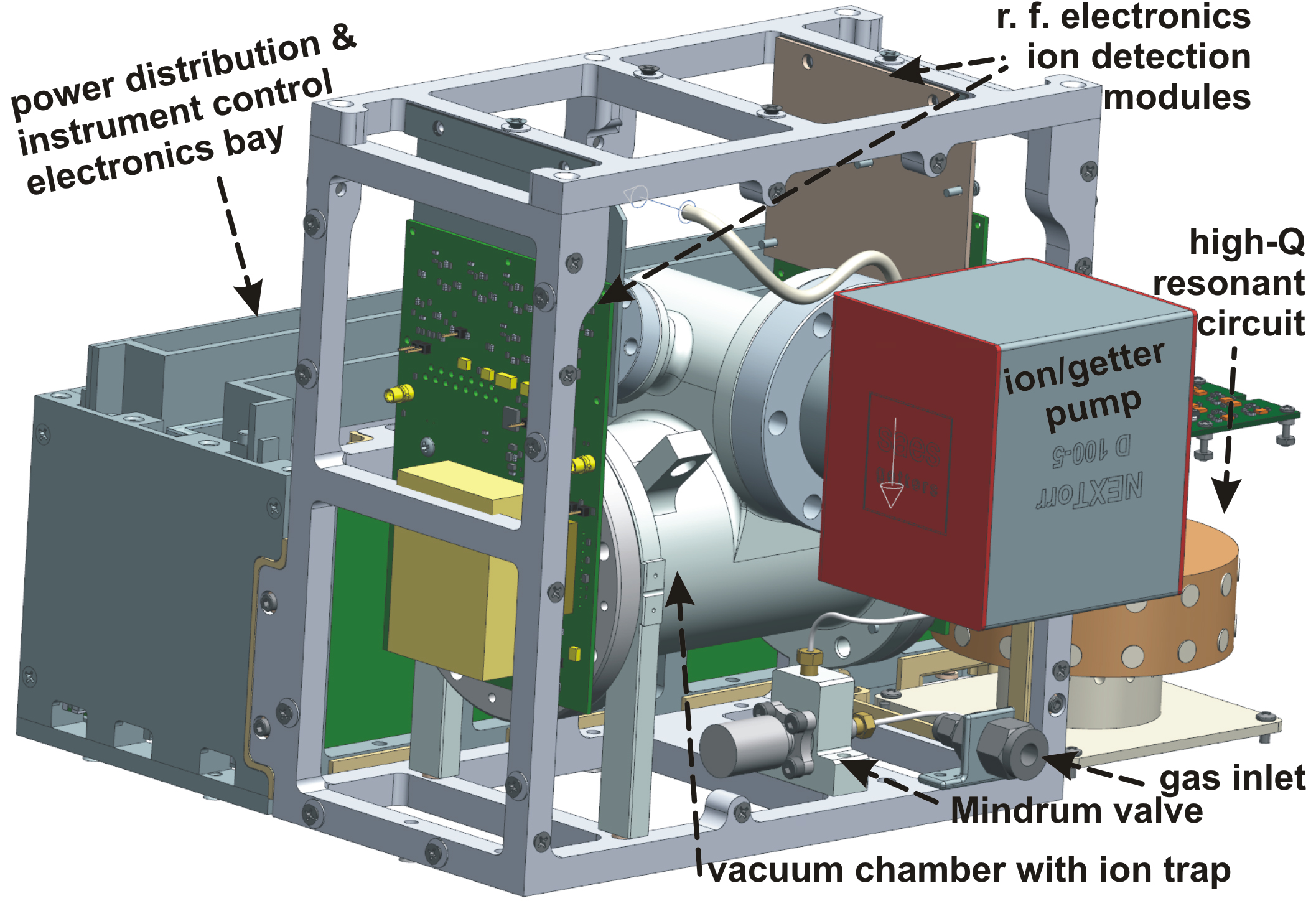For simplicity we neglect contribution of N₂ viscosity in CO₂/N₂ binary mixture because N₂ enters the mixture at 3.5%. Instead, when passing through the sampling inlet shown in Figure 1, all minor species are regarded as fully dissolved in the dominant CO₂ matrix. By maintaining the sampling inlet flow at room temperature, the characteristic pressure p_c in Equation (4) is due to CO₂ and will change only with the tube diameter d. For the fixed dimensions of the sampling tube, the pV-flow $Q_{d,L}^m$ in Equation (3) will predominantly change with the inlet pressure p_in and the type of chemical species m being transferred.

3.3.3. Computation of Pumping Speeds

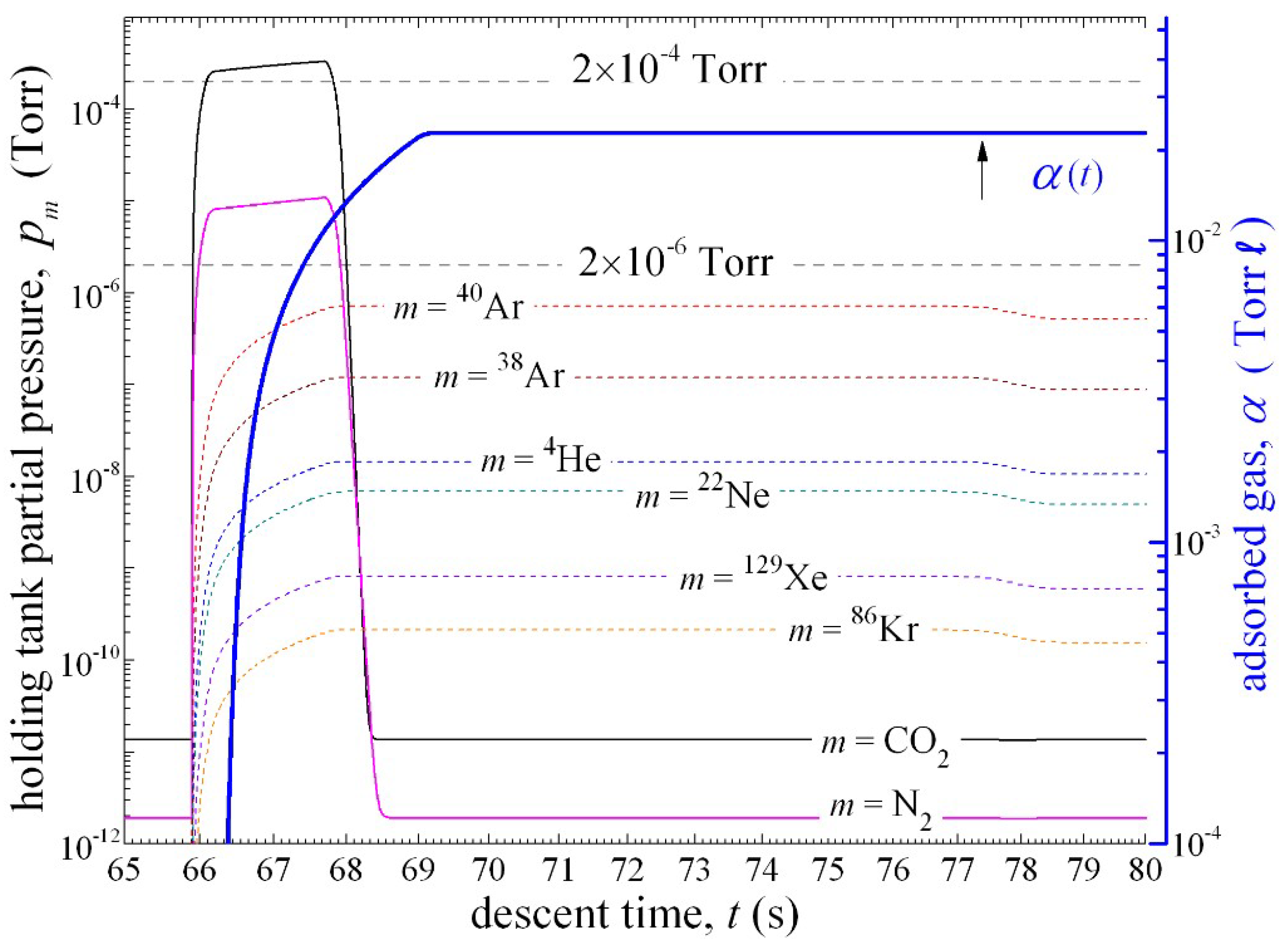
The mass-dependent pV-flow $Q_{d,L}^m$ through the SST of sampling inlet is driven by the time-dependent pressure difference between the head of the sampling inlet and the holding tank. Thus, the time-dependent pV-flow is calculated with help of Equation (3), (4), such that the M₁ valve remains open during 2 s of sampling and admits 23 × 10⁻³ Torrℓ of atmosphere into the holding tank, see Figure 3. At the same time, downstream from the holding tank, the Mindrum valve M₂ remains closed, see Table 4.

The holding tank is continuously pumped by the CapaciTorr D100 getter pump. We assume, without loss of generality, that the holding tank temperature T = 300 K is unchanged by admiting hot/fast sample. This assumption is supported by the following consideration. The holding tank has the specific heat capacity of 0.5 Jg⁻¹ K⁻¹ [57] and during 2 s of sampling at ~10 km/s it will accommodate about 7.4 × 10¹⁷ molecules. Admitted molecules may exchange at most 3.2 J of its kinetic energy in collisions with holding tank walls, and consequently may raise the temperature of the system by at most 0.4 K.

The CapaciTorr D100 pumping speeds $S^m(\alpha (t))$ as a function of already adsorbed material $\alpha (t)$ have been previously measured by Hogan & Malyshev [45] but only for a few common getterable gases (N₂, H₂, CO, CO₂, CH₄). Pumping speed for O₂ (m = 32) can be found in the NEXTorr D100-5 user manual. In general, hydrogen and its isotopes are sorbed reversibly; CO, CO₂, O₂, and N₂ are chemisorbed irreversibly; H₂O and hydrocarbons are sorbed in a combination of slow reversible and irreversible processes, whereas inert gases are not sorbed at all and are enriched relative to the residual gas. Details about simulated pumping speeds of chemically-active species as a function of already adsorbed material will be published elsewhere.

3.4. Composition of Sample Volume

The composition of sample volume is the output from the simulated SA&H module, see Figure 2, and consists of an inventory of all molecular species present in the sample as a function of time. The time-dependent number of molecules $N_m$ of mass $m$ inside the holding tank of volume $V_{\mathrm{h}}$ is obtained as numerical solution to the set of coupled first order differential equations,

$$\frac{d{N}_m}{dt}=\frac{Q_{d,L}^m(t)}{k_{\mathrm{B}}T}+(\frac{p_{\mathrm{b}}^m}{k_{\mathrm{B}}T}-\frac{N_m}{V_{\mathrm{h}}})\times S^m(\alpha (t)),N_m(t\le 65.9\mathrm{s})=\frac{p_{\mathrm{b}}^m{V}_{\mathrm{h}}}{k_{\mathrm{B}}T},$$

(5)

where the molecular mass $m$ takes values for isotopes of all chemical species found in Table 2 and Table 3. Coupling is governed by the instantaneous values of adsorption $\alpha \alpha (tt)$, which represents amount of already sorbed material due to all species. The sampling inlet, holding tank, and vacuum chamber (with the volume of $V{V}_{\mathrm{ch}}$ = 0.371ℓ) are all maintained at room temperature, $TT$ = 300 K.

At the start of atmospheric measurements, see Table 4, the initial background partial pressures $p_{\mathrm{b}}^m$ are assumed to be zero except for the previously discussed residual gas molecules. The solution of Equation (5) for the carbon dioxide $m m$ = CO₂ in the form of the time-dependent partial pressure $p_m(t)=N_m(t)k_{\mathrm{B}}T/V_{\mathrm{h}}$ is further detailed in Figure 3. At the instant when the M₂ valve is closed, the total amount of adsorbed gas is $\alpha \alpha (69.7ss)$ ≈ 23 ×10⁻³ Torr ℓ, which will degrade the pumping speed for CO₂ to 88% of its unsaturated value; similar degradation in pumping speed is seen across other getterable chemical species, such are for example N₂ (85%) and S₈(92%). During the static measurement of noble gases, ion pump is turned off and the pumping speed for all noble gases is assumed to be zero. Figure 3 illustrates that partial pressures of the most abundant noble gas isotopes will never exceed the 2.7 × 10⁻⁴ Pa limit. If needed, this limit can be lowered most efficiently by reducing the inner diameter d of the sampling inlet tube. As illustrated in Figure 3, after opening the M₂ valve ($t t$ = 77.5 s), the sample will expand into the vacuum chamber and noble gas partial pressures will reach equilibrium levels that are $\frac{V{V}_{\mathrm{h}}}{V{V}_{\mathrm{h}}+V{V}_{\mathrm{ch}}}$ ≈ 0.73 times the previous value.

3.5. Model of the QIT-MS Sensor

Modeling the performance of the QIT-MS sensor is the next phase in the simulation flow chart given in Figure 2. The composition of the sample volume is previously obtained in the SA&H module, and is used here as an input to the simulation of the QIT-MS sensor capabilities. The Capacitor D100 getter pump attached to the holding tank and the NEXTorr D100-5 getter pump attached to the vacuum chamber efficiently adsorb any residual chemically-active species except noble gases.

Shortly after the M₂ is open, residual partial pressures of chemically-active species in both the holding tank and the vacuum chamber will assume a new equilibrium levels listed in

Table 5. Equilibrated partial pressures of residual background gases.

Species	Pressure (Pa)	Species	Pressure (Pa)
CO2	1.87 × 10−9	H2O	1.87 × 10−9
N2	2.67 × 10−10	H2	2.67 × 10−8
CO	1.47 × 10−9	-	-

. The new background pressure will be the volume-weighted average of background pressures in the holding tank and in the vacuum chamber prior to the opening of the M₂ valve. For simplicity we will assume that the new background pressure remains unchanged as indicated in Figure 3 for CO₂ and N₂, and reported in Table 5 for other background species. At the same time noble gas isotopes in the sample volume will remain enriched at relative levels established previously in the holding tank as listed in

Table 6. Equilibrated partial pressures $p_m$ of noble gases isotopes during static measurement.

Isotope		Pressure (Pa)	Isotope		Pressure (Pa)
Ne	20	7.21 ×10−6	He	3	1.93 × 10−10
	21	1.87 × 10−8		4	1.41 × 10−6
	22	6.63 × 10−7	Xe	124	3.33 × 10−10
Ar	36	6.04 × 10−5		126	2.93 × 10−10
	38	1.17 × 10−5		128	5.87 × 10−9
	40	6.93 × 10−5		129	7.87 × 10−8
Kr	80	1.60 × 10−8		130	1.17 × 10−8
	82	5.60 × 10−8		131	6.00 × 10−8
	83	3.33 × 10−8		132	7.33 × 10−8
	84	1.17 × 10−7		134	2.67 × 10−8
	86	2.00 × 10−8		136	2.13 × 10−8

. The total pressure of all noble gas isotopes is equilibrated at 1.49 × 10⁻⁴ Pa.

The least abundant isotopes ³He, ¹²⁴Xe, and ¹²⁶Xe contribute to the sample volume in amounts that are five orders of magnitude smaller than the ⁴⁰Ar and ³⁶Ar contributions. Accurate detection of trace amounts of isotopes in the presence of other dominant isotopes in a short period of time represents a challenge, as it requires a sufficient counting of statistics of rare events, namely, in the nominal operation of the QIT-MS sensor all ions are indiscriminately created, stored, and recorded 20 times per second [15]. However, as previously discussed in Section 2.2, the QIT-MS sensor operates with peak performance given that the following two conditions are fulfilled: (a) the space charge effects due to ion-ion interactions are negligible, and (b) ion collisions with neutral molecules are rare. We determined empirically [15] that both conditions are satisfied when the total number of ions within the trap does not exceed 5000 at any given moment and the pressure does not exceed 2.7 × 10⁻⁴ Pa limit.

Therefore, in the nominal operation, the repetition rate of 20 duty cycles per second amounts to at most 100,000 ions being analyzed each second. Note that the duration of 50 ms for the single cycle has been chosen to provide mass resolution of 800 at 140 u, which will fully separate individual isotope peaks in xenon [15]. The mass resolution scales with the square root of analysis time. For example, if the duration of the trapping phase is kept at 6.12 ms, see Figure 1c, but the duration of a duty cycle is reduced from 50 ms to 25 ms, the count rate will double and the mass resolution will be 52% lower. Lower mass resolution causes neighboring isotope peaks to overlap and counting integrated counts under the single peak becomes unreliable metrics for accurate determination of isotopic ratios [15].

For each individual cycle we can shorten or prolong the duration of the ionization phase on demand, effectively adjusting the number of stored ions to below 5000. It is evident from Table 6 that the ³⁶Ar and ⁴⁰Ar isotopes will contribute 85.8% of all created ions. On the other hand, the most abundant krypton isotope ⁸⁴Kr will be created only 0.08% of the time, and thus, will contribute 4 ± 2 ions in each 50 ms duty cycle. To remedy this problem, we make use of resonant ejection technique [16], such that during the ionization phase we simultaneously destabilize trajectories of select m/q ions.

This is done by adding two additional low-amplitude phase-inverted RF drives to the QIT-MS-S. For trapping conditions used in this study, the frequencies for removing ³⁶Ar⁺ and ⁴⁰Ar⁺ ions are 108.2 kHz and 96.9 kHz, respectively. The resonant ejection method is used in 19 out of 20 duty cycles to suppress ³⁶Ar⁺ and ⁴⁰Ar⁺ ions by factor of 100. We note that doubly-charged ³⁶Ar²⁺ and ⁴⁰Ar²⁺ ions will not be affected. The last duty cycle out of 20 duty cycles is carried out without the resonant ejection, but with much shorter ionization phase where only the most abundant isotopes are created and trapped. In this hybrid operation mode, we effectively improve the dynamic range of the instrument.

The starting point for calculation of the composition of the detected ion cloud is the neutral molecular/atomic composition represented with individual partial pressures $p_m(t)$, see Table 6. Using the trap sensitivity s and the probability π_m for confinement and detection of m/q ions, we can calculate the number of ions being detected for each individual measurement cycle. Distribution of ionization rates of the sample species was obtained by using the recommended absolute total cross sections for electron-impact ionization of the noble gases [58]. For example, by using the electron beam with 70 eV energy, He²⁺ and Ne²⁺ will not be created, whereas the Ar¹⁺/Ar²⁺, Kr¹⁺/Kr²⁺, and Xe¹⁺/Xe²⁺ ion number ratios are estimated to be 18.4, 87.3, and 12.1 respectively. During 6.12 ms of the ion trapping phase, all created ions in the first 5 ms were confined using the RF potential with constant amplitude of 96.1 V. In the analysis phase, the RF amplitude was linearly ramped to 1049 V in 43.88 ms. For each ion we register its position, velocity, and time of detection. Initial ions are randomly generated during the first 5 ms of the trapping phase and uniformly distributed inside the cylinder (4 mm long axially and 1 mm wide radially, see inset in Figure 1a) placed in the center of the QIT-MS sensor. In the present study the 4 mm axial spread of the initial ion cloud is chosen to benchmark the effect of overlap among neighboring isotopes in the mass spectrum. Initial thermal velocities of created ions are randomly drawn from the Maxwell-Boltzmann distribution at the temperature of 300 K.

Immediately after their creation, ions are propagated through the RF quadrupole electric field using 1 ns time steps. Ion velocities and positions are updated by modified Verlet algorithm [16]. Propagation of ions is stopped if the duty cycle has ended, a collision with electrode surfaces has been recorded, or ion has been detected. At the end of every duty cycle, detected ions are added to the final ion cloud and post-processed to yield a measured mass spectrum. By comparing the number of initial ions of given m/q and the corresponding number of detected ions, we calculate the detection probability π_m.

Table 7. Expected noble gas (ng) and background (bg) count rates in 20 nominal 50 ms duty cycles, equivalent to 1 s of measurement time during probe flyby. In this example the average number of ions created in a single duty cycle is 4970. Precision is defined as standard uncertainty of the total number of counts expected to be accumulated for a given isotope in 40 min of measurement. Detection probability of isotope ion with m/q is denoted with π_m.

ng Isotope	Count Rate (cps)	πm	Precision (%).	ng Isotope	Count Rate (cps)	πm		Precision (%).
3He	0.122	0.7810(1)	[5.2]	124Xe	0.215	0.8053(2)		[4.0]
4He	912	0.8058(3)	[0.06]	126Xe	0.189	0.8101(9)		[4.2]
20Ne	4650	0.7332(2)	[0.03]	128Xe	3.81	0.8044(7)		[0.9]
21Ne	11.9	0.7347(4)	[0.6]	129Xe	51.06	0.8043(6)		[0.26]
22Ne	427.2	0.7384(3)	[0.1]	130Xe	7.638	0.8056(7)		[0.66]
36Ar	38929	0.7698(6)	[0.01]	131Xe	38.67	0.8071(4)		[0.29]
38Ar	7533	0.7743(5)	[0.03]	132Xe	47.58	0.8089(8)		[0.27]
40Ar	44693	0.7758(5)	[0.01]	134Xe	17.40	0.8053(7)		[0.44]
80Kr	10.38	0.7934(5)	[0.6]	136Xe	13.94	0.8086(8)		[0.49]
82Kr	36.05	0.7902(1)	[0.3]	s[cps/Pa]			6.6 ×108
83Kr	21.53	0.7914(4)	[0.4]	$p_{\mathrm{ng}}$[Pa]			1.49 ×10−4
84Kr	75.67	0.7944(6)	[0.2]	sx$p_{\mathrm{ng}}$[cps]			99263
86Kr	13.33	0.7954(9)	[0.5]	bg [cps]			141

summarizes the average number of ions being detected in 1 s of probe flyby time or equivalently in 20 subsequent measurement cycles. The total counting rate for noble gases is s×$p{p}_{\mathrm{ng}}$ = 99263 cps, which means that every second on average we are randomly sampling from the Poisson distribution 99263 ions within standard uncertainty of 315 ions. To avoid oversampling, the pool of 300 million ions has been pre-generated by the Computational Ion Trap Analyzer [16] (CITA) such that end-cap electrodes are grounded and the central ring electrode is driven by the 867.791 kHz RF potential. Sample pool of ions when ³⁶Ar⁺ and ⁴⁰Ar⁺ ions are resonantly depleted is also created by CITA program by driving the end-caps by an auxiliary phase-inverted RF potential of 0.6 V amplitude and with mixed dual frequency (108.2 kHz and 96.9 kHz).

Response of the QIT-MS instrument to neutral gas sample is accumulated in 1 s intervals by twenty random samplings of approximately 5000 ions from the final ion cloud using Poisson probability density function. As an example,

Table 8. The distribution of number of randomly created ions during 20 subsequent 50 ms duty cycles. First 19 duty cycles operate at sensitivity of 4.62 × 10⁹ cps/Pa under the active secular ejection of ³⁶Ar⁺ and ⁴⁰Ar⁺ ions, whereas the last duty cycle is set at sensitivity of 6.6 × 10⁸ cps/Pa and has no secular ejection.

Isotope	Index of 50 ms Duty Cycle
	#1	#2	#3	#4	#5	#6	#7	#8	...	#19	#20
3He	0	0	0	0	0	0	0	0	...	0	0
4He	345	295	318	320	300	335	351	366	...	337	55
20Ne	1634	1666	1665	1582	1638	1710	1666	1647	...	1665	269
21Ne	4	5	8	3	5	4	1	4	...	4	0
22Ne	147	145	138	149	161	149	143	142	...	131	23
36Ar	18	18	13	26	17	17	16	24	...	18	1975
38Ar	2724	2653	2691	2557	2719	2692	2639	2511	...	2629	394
40Ar	39	17	23	34	18	20	20	20	...	26	2339
80Kr	6	6	3	1	3	2	4	1	...	2	0
82Kr	7	13	8	22	16	14	13	18	...	12	0
83Kr	6	10	5	5	7	6	4	10	...	6	0
84Kr	17	25	27	30	26	25	30	30	...	32	3
86Kr	1	4	3	4	9	5	1	4	...	7	0
124Xe	0	0	0	0	0	0	0	0	...	0	0
126Xe	0	0	0	0	0	0	0	0	...	0	0
128Xe	0	2	0	1	1	2	2	0	...	0	0
129Xe	23	14	17	13	14	19	21	20	...	21	3
130Xe	3	5	0	0	6	1	0	2	...	5	0
131Xe	13	16	13	11	13	10	7	16	...	10	1
132Xe	18	14	15	20	18	20	13	21	...	11	5
134Xe	3	6	9	6	4	7	2	6	...	6	0
136Xe	5	6	4	2	3	4	0	3	...	1	0
Counts:	5013	4920	4960	4786	4978	5042	4933	4845	...	4923	5067

illustrates the distribution of detected ions in twenty subsequent duty cycles. Sampled mass spectra can be co-added in time intervals of up to 40 min in duration; then we extract ion detection times and mass-to-charge (m/q) ratios and perform a linear regression analysis by computing the slope and the intercept of the regression line through data. This procedure establishes the linear correspondence between the ion’s detection time and its m/q value. By counting how many ions of certain m/q value will contribute to the given m/q bin width, we generate histogram plots representing a mass spectrum, see Figure 1. For example, 2724 counts for ³⁸Ar⁺ that are detected in the first duty cycle of Table 8 will be all distributed in 15 bins each 1 × 10⁻² u wide. In the nominal QIT-MS data acquisition setting, after 40 min of operation we will accumulate a count matrix with 40 × 60 × 20 = 48,000 rows (duty cycles) such that each row is representing a full mass spectrum with 16,000 mass bins. Each row in the data matrix is statistically independent from any other row, which is a direct consequence of Monte-Carlo simulation approach when creating the ion cloud for each duty cycle. Namely, initial ion positions, thermal velocities, and creation times will always be different between duty cycles, and detected mass spectra will be statistically different.

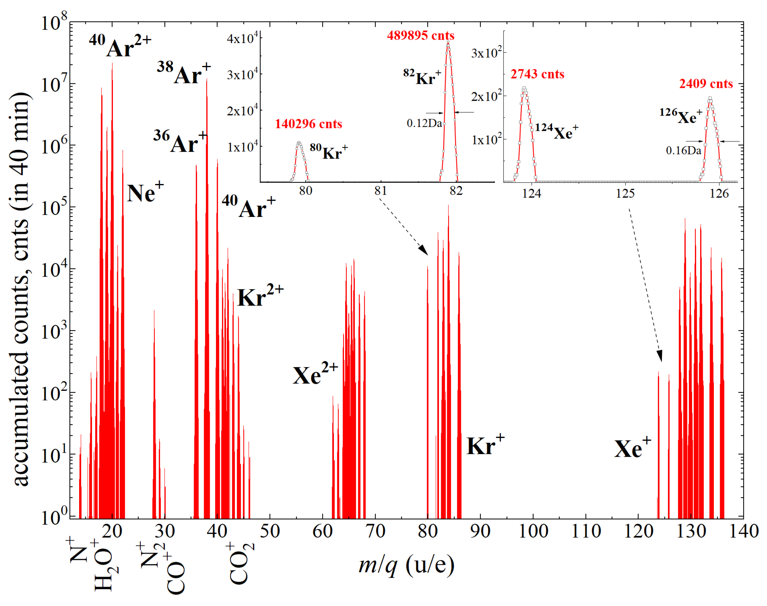
We note that collisions among ions and neutral molecules are neglected as rare events [15], but can be included in propagation of ions to study the spread and broadening of line shapes of each mass peak. Figure 4 illustrates the part of synthetic mass spectrum accumulated in 40 min of static measurements of noble gas isotopes. Data matrix has been histogrammed in 1 × 10⁻² u wide bins. For comparison, the typical mass spectra provided by previously flown mass-hopping spectrometer [59] are of 1u resolution.

4. Analysis of Isotopic Abundances in Noble Gases

To extract isotope abundances from the synthetic mass spectrum illustrated in Figure 4, we use the random walk algorithm developed for deconvolution of elution profiles of volatile organic compounds [60]. The presence of each isotope in the mass spectrum is probed in random fashion based on unique electron impact ionization probabilities to generate singly- and doubly-charged ions during the ionization phase. Each isotope will contribute at most two lines in the mass spectrum, centered at m/2q and m/q mass bins, respectfully. For example, in Figure 4 singly-charged Xe⁺ isotopes at 124 u–136 u will be accompanied by doubly charged Xe²⁺ isotopes found at 62 u–68 u. Note that the ratio of singly-charged to doubly-charged argon isotopes is reverted due to the selective resonant suppression of ³⁶Ar⁺ and ⁴⁰Ar⁺ ions. Even if ³⁸Ar⁺ ions are also resonantly suppressed, there is still sufficient counting statistics of doubly-charged argon isotopes to accurately determine ³⁶Ar/⁴⁰Ar and ³⁸Ar/⁴⁰Ar ratios.

We note that detected ions will form asymmetric mass line profiles [15] with shapes that depend on specific trapping conditions, RF amplitude scan function, and accumulated counting statistics. Insets in Figure 4 show the line shapes of two least abundant krypton and xenon isotopes. Ion detector response to a harsh radiation environment is not included in the present study. Detectors dark current will present itself as a random noise signal distributed over 16,000 mass channels. However, the presence of random noise in spectrum will be filtered out by the deconvolution procedure, since it relies only on well-defined patterns to fit the whole mass lines profile and will smooth out sporadic fluctuations in data points. The measurement of helium isotopes requires different RF voltage scan function across 2.5 u–5 u mass region, and is not shown in Figure 4. Namely, confinement of helium ions was carried out during 6.12 ms in RF potential with constant amplitude of 17.5 V, whereas in the analysis phase RF amplitude was linearly ramped to 35V in 43.88 ms. Resulting mass line shapes for ³He and ⁴He are well separated and with FWHM of 3.3 × 10⁻³ u (not shown in Figure 4), which is consistent with previous experimental FWHM of 8 × 10⁻³ u when separating ⁴He from much closer D₂ peak [16]. Low residual background pressure of water vapor is sustained by getter pumps and ensures negligible interference of HD/D₂ fragment ions from water to the ³He/⁴He isotopes.

In deconvolution procedure, a trial linear combination of mass spectra of all species is randomly formed and evaluated against the synthetic mass spectrum similar to those found in Figure 4. Mixing coefficients for each isotope in this linear combination are iteratively varied until the absolute value of the difference between the two spectra is minimized or prescribed number of trials is exhausted.

Table 9. Deconvolution efficiency for noble gases in the mass spectrum in Figure 4. Parentheses contain standard uncertainties for the number of created ions inherited from detection probabilities π_m found in Table 7.

Isotope		Detected Ions (Nd)	Retrieved Ions (Nr)	Created Ions (Nr/πm)	Isotope		DetectedIons (Nd)	RetrievedIons (Nr)	Created Ions (Nr/πm)
Ne	20	74762700	74759700	101964483(20393)	He	3	2177	2176.86	2787(1)
	21	190763	190755	259631(104)		4	15351560	15351595	19050870(5715)
	22	6865110	6865360	9297979(2789)	Xe	124	3374	3373.97	4189(1)
Ar	36	5556000	5555680	7217378(4330)		126	2963	2962.87	3657(3)
	38	121091000	121098000	156399086(78200)		128	60963	60960	75781(53)
	40	6378580	6378920	8221997(4111)		129	819946	819921	1019414(612)
Kr	80	166345	166337	209662(105)		130	122355	122350	151884(106)
	82	578673	578655	732329(73)		131	620754	620740	769126(308)
	83	345503	345497	436590(175)		132	763928	763915	944373(755)
	84	1215360	1215320	1529914(918)		134	279131	279119	346622(243)
	86	213671	213662	268632(242)		136	223586	223420	276293(221)

illustrates the accuracy of peak deconvolution procedure by comparing a-priori known number of ions of each isotope (“detected ions”) with the number of ions deconvoluted (“retrieved ions”) using the random walk algorithm [60]. The error of the deconvolution procedure is much smaller than the uncertainty of Poisson counting statistics, ensuring that the longer measurement times will yield more accurate results. For each isotope m/q ion, the number of detected ions (N_d) is proportional to the number of created ions. The proportionality factor is a complex function of trapping conditions and was previously summarized in Table 7 as the detection probability, π_m. Therefore, the estimate of initially created ions for each isotope reported in Table 9 is simply the ratio of the number of retrieved ions N_r and corresponding detection probabilities π_m.

Response of the QIT-MS instrument to the model noble gas composition of Venus’s atmosphere is obtained by close inspection of Table 2 and Table 9. For example, the ³He/⁴He isotope ratio at the sampling inlet is approximately 135 × 10⁻⁶. If this ratio is calculated from the number of created ions found in Table 9, then the approximate value of 146 × 10⁻⁶ is obtained, resulting in an absolute error of 8.1% for ³He/⁴He. Similarly, absolute errors for isotope ratios for other trace isotopes are: ~0.6% (²¹Ne/²²Ne), ~0.7% (⁸⁰Kr/⁸⁶Kr), ~0.7% (¹²⁴Xe/¹²⁶Xe), ~0.8% (³⁶Ar⁺/⁴⁰Ar⁺) and ~0.13% (³⁸Ar²⁺/⁴⁰Ar²⁺), respectively. By co-adding the mass spectra for all isotopes of a given element, we can estimate the abundance ratios among different species. This approach yields absolute error of approximately 2% for He/Ne, 2.2% for the Kr/Xe ratio and approximately 8% for Ne/Kr ratio. Main source of absolute error in abundance ratios of different species are variable detection probabilities π_m across the investigated mass range. Note that by increasing the RF drive frequency we can effectively reduce the variability in detection probabilities π_m for all noble gas isotopes, but this will increase QIT-MS power consumption. Given the time restrictions set by mission objectives and available instrument power, we can optimize the sample transfer function in the SA&H module to provide sufficient amount of noble gas isotopes to the QIT-MS sensor, and infer the QIT-MS-I response function to the changing atmospheric composition with an absolute error better than 9% for all noble gas species. On the other hand, isotopic ratios for a single species (except for helium) are retrievable with an absolute error better than 1%.

5. Conclusions

We have demonstrated use of a computational platform to quantify the response of the QIT-MS instrument in a simulated Venus atmosphere ‘skimmer’ probe mission. Each phase in the simulated experiment is described in detail, providing the reader with an insight into achievable outcomes in support of science objectives when the mission concept is in early stages of planning. Particular attention is devoted to modeling both the sample inlet and the sample accommodation as these directly influence the composition of the sample that is being admitted into the mass spectrometer. We show that based on published data on chemical composition of Venus atmosphere and realistic probe trajectory, the QIT-MS instrument will deliver accurate isotope ratios of all noble gases. Furthermore, the QIT-MS sensor can be operated in highly-adjustable mode designed to suppress major isotopes and target primarily trace isotopes to meet science objectives of any atmospheric probe mission. Further investigation of the reaction zone formed at the sampling inlet is necessary. We will use a detailed kinetic model of chemical reaction processes based on realistic thermochemistry rates. Numerical solutions to the hypervelocity low-density high-temperature gas flow around atmospheric probe will provide answers regarding the extent to which the thermal decomposition and charge exchange between trace amounts of acidic molecules and noble gases in the CO₂/N₂ matrix may affect our capability to accurately measure isotopic ratios in noble gases.

References

1. Palmer, P.T.; Limero, T.F. Mass spectrometry in the U.S. space program: Past, present, and future. J. Am. Soc. Mass Spectrom. 2001, 12, 656–675. [Google Scholar] [CrossRef]
2. Freeman, A.; Smrekar, S. VERITAS—A Discovery-class Venus surface geology and geophysics mission. In Proceedings of the 11th Low Cost Planetary Missions Conference, Berlin, Germany, 9–11 June 2015. [Google Scholar]
3. NRC. Vision and Voyages for Planetary Science in the Decade 2013–2022; The National Academies Press: Washington, DC, USA, 2011. [Google Scholar]
4. Owen, T. Solar composition of icy planetesimals: A new source for comet nuclei? Highlights of Astronomy. In Proceedings of the 25th General Assembly of the IAU, Sydney, Australia, 13–26 July 2003; Volume 13. [Google Scholar]
5. Fischer, D.A.; Valenti, J. The Planet-Metallicity Correlation. Astrophys. J. 2005, 622, 1102–1117. [Google Scholar] [CrossRef]
6. Klahr, H.; Bodenheimer, P. Formation of Giant Planets by Concurrent Accretion of Solids and Gas Inside an Anticyclonic Vortex. Astrophys. J. 2006, 639, 432–440. [Google Scholar] [CrossRef]
7. Owen, T.; Bar-Nun, A. Cometary Contributions to Planetary Atmospheres. In Exobiology: Matter, Energy, and Information in the Origin and Evolution of Life in the Universe; Chela-Flores, J., Raulin, F., Eds.; Springer: Berlin/Heidelberg, Germany, 1998; pp. 269–273. [Google Scholar]
8. Kallenbach, R.; Encrenaz, T.; Geiss, J.; Mauersberger, K.; Owen, T.C.; Robert, F. Element Abundances and Isotope Ratios in the Giant Planets and Titan. In Solar System History from Isotopic Signatures of Volatile Elements; Kallenbach, R., Encrenaz, T., Geiss, J., Mauersberger, K., Owen, T.C., Robert, F., Eds.; Kluwer Academic Publishers: Dordrecht, The Netherlands, 2003; pp. 121–138. [Google Scholar]
9. Owen, T.; Bar-Nun, A. Comets, impacts and atmospheres II. Isotopes and noble gases. AIP Conf. Proc. 1995, 341, 123. [Google Scholar]
10. Owen, T. Atmospheric Probes: Needs and Prospects. In Proceedings of the International Workshop on Planetary Probe Atmospheric Entry and Descent Trajectory Analysis and Science, Lisbon, Portugal, 6–9 October 2003. [Google Scholar]
11. Atreya, S.K.; Wong, A.S. Coupled Chemistry and Clouds of the Giant Planets—A Case for Multiprobes. In The Outer Planets and Their Moons; Encrenaz, T., Kallenbach, R., Owen, T.C., Sotin, C., Eds.; Springer Publishers: Berlin/Heidelberg, Germany; New York, NY, USA, 2005; pp. 121–136. [Google Scholar]
12. Niemann, H.B.; Atreya, S.K.; Carignan, G.R.; Donahue, T.M.; Haberman, J.A.; Harpold, D.N.; Hartle, R.E.; Hunten, D.M.; Kasprzak, W.T.; Mahaffy, P.R.; et al. The composition of the Jovian atmosphere as determined by the Galileo probe mass spectrometer. J. Geophys. Res. Planets 1998, 103, 2156–2202. [Google Scholar] [CrossRef]
13. Pauken, M.; Kolawa, E.; Manvi, R.; Sokolowski, W.; Lewis, J. Pressure Vessel Technology Developments. In Proceedings of the 4th International Planetary Probe Workshop, Pasadena, CA, USA, 27–30 June 2006. [Google Scholar]
14. Chassefière, E.; Wieler, R.; Marty, B.; Leblanc, F. The evolution of Venus: Present state of knowledge and future exploration. Planet. Space Sci. 2012, 63–64, 15–23. [Google Scholar] [CrossRef]
15. Madzunkov, S.M.; Nikolić, D. Accurate Xe isotope measurement using JPL ion trap. J. Am. Soc. Mass Spectrom. 2014, 25, 1841–1852. [Google Scholar] [CrossRef]
16. Nikolić, D.; Madzunkov, S.M.; Darrach, M.R. Computer Modeling of an Ion Trap Mass Analyzer, Part I: Low Pressure Regime. J. Am. Soc. Mass Spectrom. 2015, 26, 2115–2124. [Google Scholar] [CrossRef] [PubMed]
17. Darrach, M.; Madzunkov, S.; Schaefer, R.; Nikolic, D.; Simcic, J.; Kidd, R.; Neidholdt, E.; Pilinski, M.; Jaramillo-Botero, A.; Farley, K. The Mass Analyzer for Real-time Investigation of Neutrals at Europa (MARINE). In Proceedings of the IEEE Aerospace Conference, Big Sky, MT, USA, 7–14 March 2015. [Google Scholar]
18. Mahieux, A.; Vandaele, A.C.; Robert, S.; Wilquet, V.; Drummond, R.; Montmessin, F.; Bertaux, J.L. Densities and temperatures in the Venus mesosphere and lower thermosphere retrieved from SOIR on board Venus Express: Carbon dioxide measurements at the Venus terminator. J. Geophys. Res. 2012, 117, E07001. [Google Scholar] [CrossRef]
19. Brecht, A.S.; Bougher, S.W.; Gérard, J.C.; Soret, L. Atomic oxygen distributions in the Venus thermosphere: Comparisons between Venus Express observations and global model simulations. Icarus 2012, 217, 759–766. [Google Scholar] [CrossRef]
20. Von Zahn, U.; Fricke, K.H.; Hunten, D.M.; Krankowsky, D.; Mauersberger, K.; Nier, A.O. The Upper Atmosphere of Venus during Morning Conditions. J. Geophys. Res. 1980, 85, 7829–7840. [Google Scholar] [CrossRef]
21. Jacobson, M.Z. Fundamentals of Atmospheric Modeling, 2nd ed.; Cambridge University Press: Cambridge, UK, 2005; p. 528. [Google Scholar]
22. Benvenuti, C. Molecular Surface Pumping: The Getter Pumps; CAS—CERN Accelerator School: Snekersten, Denmark, 1999; pp. 43–50. [Google Scholar]
23. Madzunkov, S.; Bae, B.; Simcic, J.; Rellergert, W.; Gill, J.; Schaefer, R.; Neidholdt, E.L.; Nikolic, D.; Kidd, R.; Darrach, M. Progress Report on the Spacecraft Atmosphere Monitor’s Development Model. In Proceedings of the 48th International Conference on Environmental Systems, Albuquerque, NM, USA, 8–12 July 2018. [Google Scholar]
24. Smith, J.T. Miniaturized Double Latching Solenoid Valve. U.S. Patent 20,090,078,900, 26 March 2009. [Google Scholar]
25. Justh, H.L.; Cianciolo, A.M.D. Venus Global Reference Atmospheric Model Status and Planned Updates. In Proceedings of the Venus Modeling Workshop, Cleveland, OH, USA, 9–11 May 2017. NTRS report M17-5876. [Google Scholar]
26. Krasnopolsky, V.A. A photochemical model for the Venus atmosphere at 47-112 km. Icarus 2012, 218, 230. [Google Scholar] [CrossRef]
27. Krasnopolsky, V.A. Chemical kinetic model for the lower atmosphere of Venus. Icarus 2007, 191, 25. [Google Scholar] [CrossRef]
28. Lietzke, M.H.; Mullins, C. The thermal decomposition of carbon dioxide. J. Inorg. Nucl. Chem. 1981, 43, 1769–1771. [Google Scholar] [CrossRef]
29. NIST. NIST-JANAF Thermochemical Tables, NIST Standard Reference Database 13. 1998. Available online: https://janaf.nist.gov (accessed on 23 March 2018).
30. Warr, O.; Rochelle, C.A.; Masters, A.; Ballentine, C.J. Determining noble gas partitioning within a CO2-H2O system at elevated temperatures and pressures. Geochim. Cosmochim. Acta 2015, 159, 112–125. [Google Scholar] [CrossRef]
31. Zahnle, K.J.; Gacesa, M.; Catling, D.C. Strange messenger: A new history of hydrogen on Earth, as told by Xenon. Geochim. Cosmochim. Acta 2019, 244, 56–85. [Google Scholar] [CrossRef]
32. Cortez, A.F.; Santos, M.A.; Veenhof, R.; Patra, R.N.; Neves, P.N.; Santos, F.P.; Borges, F.I.; Conde, C.A. Experimental ion mobility measurements in Xe-CO2. J. Instrum. 2017, 12, P06012. [Google Scholar] [CrossRef]
33. Ruscic, B.; Pinzon, R.E.; Von Laszewski, G.; Kodeboyina, D.; Burcat, A.; Leahy, D.; Montoy, D.; Wagner, A.F. Active Thermochemical Tables: Thermochemistry for the 21st Century. J. Phys. Conf. Ser. 2005, 16, 561–570. [Google Scholar] [CrossRef]
34. Dimmock, A.P.; Balikhin, M.A.; Krasnoselskikh, V.V.; Walker, S.N.; Bale, S.D.; Hobara, Y. A statistical study of the cross-shock electric potential at low Mach number, quasi-perpendicular bow shock crossings using Cluster data. J. Geophys. Res. Space Phys. 2012, 117, A02210. [Google Scholar] [CrossRef]
35. Hoffman, J.H.; Hodges, R.R.; Donahue, T.M.; McElroy, M.B. Composition of the Venus lower atmosphere from the Pioneer Venus mass spectrometer. J. Geophys. Res. 1980, 85, 7882–7890. [Google Scholar] [CrossRef]
36. Hoffman, J.H.; Oyama, V.I.; Zahn, U. Measurements of the Venus Lower Atmosphere Composition: A Comparison of Results. J. Geophys. Res. 1980, 85, 7871–7881. [Google Scholar] [CrossRef]
37. Wieler, R. Noble gases in the solar system. Rev. Mineral. Geochem. 2002, 47, 21. [Google Scholar] [CrossRef]
38. Fegley, B. Atmospheric evolution, Venus. In The Encyclopedia of Paleoclimatology and Ancient Environments; Gornitz, V., Ed.; Kluwer Academic Publishers: Dordrecht, The Netherlands, 2009; pp. 75–83. [Google Scholar]
39. Donahue, T.M.; Hoffman, J.H.; Hodges, R.R. Krypton and xenon in the atmosphere of Venus. Geophys. Res. Lett. 1981, 8, 513. [Google Scholar] [CrossRef]
40. de Laeter, J.R.; Böhlke, J.K.; De Bièvre, P.; Hidaka, H.; Peiser, H.S.; Rosman, K.J.; Taylor, P.D. Atomic Weights of the Elements Review 2000. Pure Appl. Chem. 2003, 75, 683. [Google Scholar] [CrossRef]
41. Wieser, M.E.; Holden, N.; Coplen, T.B.; Böhlke, J.K.; Berglund, M.; Brand, W.A.; De Bièvre, P.; Gröning, M.; Loss, R.D.; Meija, J.; et al. Atomic Weights of the Elements 2011. Pure Appl. Chem. 2013, 85, 1047. [Google Scholar] [CrossRef]
42. Hugentobler, E.; Loliger, J. A General Approach to Calculating Isotope Abundance Ratios in Mass Spectroscopy. J. Chem. Educ. 1972, 49, 610. [Google Scholar] [CrossRef]
43. Pfeiffer Vacuum GmbH. Influences in real vacuum systems. In The Vacuum Technology Book; Norm Electronics Ltd.: Athina, Greece, 2018; Volume 2, p. 20. [Google Scholar]
44. SAES Group. The CapaciTorr® D 50, D 100 and D 200, D.VS.110.4.16. Available online: https://www.saesgetters. com/sites/default/files/CapaciTorr%20Products%20Datasheets.pdf (accessed on 11 November 2017).
45. Hogan, B.T.; Malyshev, O.B. Evaluation test of NEXTorr D 100-5 pump, Cockcroft Institute Report 13-47 2013. Available online: https://epubs.stfc.ac.uk/work/10795577 (accessed on 27 June 2017).
46. Jousten, K. Handbook of Vacuum Technology; Wiley-VCH: Weinheim, Germany, 2016; p. 139. [Google Scholar]
47. Fryer, G.M. A Theory of Gas Flow Through Capillary Tubes. Proc. R. Soc. Lond. 1966, 239, 329–341. [Google Scholar]
48. Ely, J.F.; Magee, J.W.; Haynes, W.M. Thermophysical Properties for Special High. CO2 Content Mixtures; Gas Processors Association: Awali, Bahrain, 1987. [Google Scholar]
49. Ouyang, L.-B. New Correlations for Predicting the Density and Viscosity of Supercritical Carbon Dioxide Under Conditions Expected in Carbon Capture and Sequestration Operations. Open Pet. Eng. J. 2011, 4, 13–21. [Google Scholar] [CrossRef]
50. Fenghour, A.; Wakeham, W.A.; Vesovic, V. The Viscosity of Carbon Dioxide. J. Phys. Chem. Ref. Data 1998, 27, 31–44. [Google Scholar] [CrossRef]
51. Span, R.; Wagner, W. A New Equation of State for Carbon Dioxide Covering the Fluid Region from the Triple-Point Temperature to 1100 K at Pressures up to 800 MPa. J. Phys. Chem. Ref. Data 1996, 25, 1509–1596. [Google Scholar] [CrossRef]
52. Sovová, H.; Prochazka, J. Calculations of Compressed Carbon Dioxide Viscosities. Ind. Eng. Chem. Res. 1993, 32, 3162–3169. [Google Scholar] [CrossRef]
53. Hanley, H.J.M. The Viscosity and Thermal Conductivity Coefficients of Dilute Argon, Krypton, and Xenon. J. Phys. Chem. Ref. Data 1973, 2, 619–642. [Google Scholar] [CrossRef]
54. Cole, W.A.; Wakeham, W.A. The Viscosity of Nitrogen, Oxygen, and Their Binary Mixtures in the Limit of Zero Density. J. Phys. Chem. Ref. Data 1985, 14, 209–226. [Google Scholar] [CrossRef]
55. Brokaw, R.S. Viscosity of Gas. Mixtures; NASA: Washington, DC, USA, 1968. [Google Scholar]
56. Davidson, T.A. A Simple and Accurate Method for Calculating Viscosity of Gaseous Mixtures; Report of Investigations RI-9456; US Department of Interiors, Bureau of Mines: Washington, DC, USA, 1993; pp. 1–12.
57. Valencia, J.J.; Quested, P.N. Thermophysical Properties. In ASM Handbook: Casting; ASM: Almere, The Netherlands, 2008; Volume 15, pp. 468–481. [Google Scholar]
58. Rejoub, R.; Lindsay, B.G.; Stebbings, R.F. Determination of the absolute partial and total cross sections for electron-impact ionization of the rare gases. Phys. Rev. A 2002, 65, 042713. [Google Scholar] [CrossRef]
59. Waite, J.H., Jr.; Lewis, W.S.; Kasprzak, W.T.; Anicich, V.G.; Block, B.P.; Cravens, T.E.; Fletcher, G.G.; Ip, W.H.; Luhmann, J.G.; McNutt, R.L.; et al. The Cassini Ion and Neutral Mass Spectrometer (INMS) Investigation. Space Sci. Rev. 2004, 114, 113–231. [Google Scholar] [CrossRef]
60. Nikolić, D.; Madzunkov, S.M.; Darrach, M. Mass Spectra Deconvolution of Gaseous Mixtures Containing Volatile Organic Compounds. In Proceedings of the 48th International Conference on Environmental Systems, Albuquerque, NM, USA, 8–12 July 2018. [Google Scholar]
Figure 1. (a) The schematic of QIT-MS-I (Quadrupole Ion Trap Mass Spectrometer Instrument) assembly consisting of: sample acquisition and handling (SA&H), mass spectrometer sensor head (QIT-MS-S), and supporting electronics module (EM); (b) Cut-through view of QIT-MS sensor; (c) standard 50 ms voltage amplitude scan functions used to ionize neutral gas samples, immediately eject dominant isotopes and confine only the trace isotopes to be analyzed. During simulations a sample of the Venus atmosphere is taken by the SA&H module where it is processed by the non-evaporable getter pump by chemically binding all but noble gases [22], and then admitted into the QIT-MS-S for analysis. The thermalizer maintains the stainless steel (SS) tube temperature at 70 °C to reduce deposition of sulfuric acid aerosols at the tube’s inner surface. The voltage amplitude scan function for the RF drive is detailed in Madzunkov & Nikolic [15].
Atmosphere 10 00232 g001
Figure 2. Modeling flow chart used in current investigation. The composition of the sample volume is calculated by the SA&H module using the composition of the Venus atmosphere and the probe trajectory. Isotopic ratios of noble gases are then calculated by QIT-MS-S module.
Atmosphere 10 00232 g002
Figure 3. Evolution of partial pressures inside the holding tank due to 2 s of sampling and after the sample has been expanded into the vacuum chamber. For valve timing sequence, see Table 4.
Atmosphere 10 00232 g003
Figure 4. Synthetic mass spectrum of heavy noble gases at 10 mu bin resolution. The residual background species are listed in Table 5 and contribute to the low count background below 47 u. The mass bin width is demonstrated in both insets as open square symbols that are centered at the top of each bin, resulting in well-defined line profiles.
Atmosphere 10 00232 g004