The Effects of the Trans-Regional Transport of PM_2.5 on a Heavy Haze Event in the Pearl River Delta in January 2015

Abstract

The Pearl River Delta (PRD), a region with the fastest economic development and urbanization in China, sometimes has severe haze pollution caused by fine particulate matter (PM_2.5). From October to April of the following year, the PRD is influenced by northerly winds, which can bring pollutants from upwind polluted regions. However, the ways that pollutants are transmitted and the contributions of trans-regional inputs are not yet clear. Observational analysis and numerical simulations are applied to explore the effect of PM_2.5 trans-regional transport during a heavy haze event occurring from 14 to 25 January 2015. The results show that northerly winds resulted in an increase in the PM_2.5 concentration in the northern PRD one day earlier than in the southern PRD. The main transport path of PM_2.5 was located at an altitude of 0.1 to 0.7 km; the maximum total transport intensity below 3 km was 9.7 × 10³ μg·m⁻²·s⁻¹; and the near-surface concentration increased by 13.7 to 34.4 μg/m³ by trans-regional transport, which accounted for 56.5% of the contribution rate on average. Southerly winds could also bring a polluted air mass from the sea to the coast, causing more severe haze in coastal regions blocked by mountains, although the overall effect is reduced pollution.

1. Introduction

The Pearl River Delta (PRD) is a typical urban agglomeration, with a land area of 42,200 km² and a very large population of 57.2 million people (residential population in 2016). During the past few decades, this region has developed rapidly in terms of both the economy and urbanization. As in other large cities, development is accompanied by haze problems mainly caused by fine particle (PM_2.5) pollution, especially from October to April of the following year [1], the dry season dominated by northerly winds.

Advection transport plays a very important role in haze events. At the local scale, pollutants can mix and accumulate within the region and even transform under favorable conditions, such as high humidity, sufficient light, and sufficient precursor conditions. Affected by the transport of atmospheric pollutants among cities, air pollution has become increasingly serious, complicated and regionalized since the 2000s [2,3,4]. According to studies by Sun et al. [5] and Yang et al. [6], secondary aerosols are the primary factors in severe haze events occurring in North China, in addition to the primary aerosol from local emissions. Moisture absorption growth of highly aging secondary aerosol due to regional transport is the leading factor on the stage when pollution growing rapidly. Regional transport is mainly located at heights of 200 to 500 m, and its contribution increases with height. In terms of large scale, regional transport can bring pollutants to downwind regions, resulting in an increase in PM_2.5 or other pollutants [7,8,9,10,11]. Wang et al. [12] studied an extreme haze event in central and eastern China that occurred in January 2013 by the Nested Air Quality Prediction Modeling System (NAQPMS). The results show that there is still significant transport within the Beijing-Tianjin-Hebei (BTH) region, even under static and stable weather conditions. Moreover, transport from outside BTH and intraregional transport among cities have similar contributions, accounting for 20% to 30% of the total transport.

The PRD is located in southern China, facing the South China Sea, and surrounded by mountains on the other three sides. Special geographic conditions make the transport conditions complex. Fan et al. [13] proposes a conceptual model of the atmospheric boundary layer in the PRD and reveals that strong background wind can purify the region, which is also demonstrated by Wu et al. [14,15], while weak wind increases the PM_2.5 concentration, especially during the dry season under stable weather conditions. In addition, local circulations, such as the sea-land breeze, mountain wind and urban heat island circulation, can also affect the air quality of the PRD if the background wind is weak. Wu et al. [16] finds that in December, 69.6% of PM_2.5 in Guangzhou (GZ) comes from outside the PRD. According to the research of Xue et al. [17,18], the contributions of external sources to annual average concentration of PM_2.5 in Guangdong Province and outside Guangdong are 72% and 28%, respectively. Sulfate, nitrate, ammonium and secondary PM_2.5 are more conducive to long-distance transport because of their smaller particle sizes [19]. Wang et al. [20] and Hu et al. [21] use the California Puff-3 (CALPUFF-3) and Community Multiscale Air Quality (CMAQ) models, respectively, to simulate and find that intercity pollutants in the PRD have mutual influence characteristics. PM₁₀ in the PRD region is mainly caused by several large cities, such as GZ, Foshan (FS), and Dongguan (DG). However, cities in the western PRD are more seriously affected by inputs from external pollution sources, such as Jiangmen (JM), Zhuhai (ZH), Zhongshan (ZS) and FS. Lyu et al. [2] designed a “zero-emission perturbation test” with the Mesoscale Model/Sparse Matrix Operator Kernel Emissions (MM5/SMOKE)-CMAQ model to simulate the spatial and temporal distributions of the main atmospheric pollutants in the PRD during 2006 and found that the long-distance transport of PM_2.5 is more significant than that of PM₁₀, especially in winter, while NO₂ is mainly from the interior of the PRD. When the PRD is controlled by a continental air mass (or coastal air mass), there are high-throughput transport inputs of PM_2.5 and SO₂ from Jiangxi (or Fujian).

The above studies mainly focus on the quantitative analysis of the contributions of trans-regional transport and cross-boundary transport, but less on the transport pathway and influence mechanism. This study uses the Weather Research and Forecasting coupled with Chemistry (WRF-Chem) online coupling model to explore the behaviors and effects of the trans-regional transport of pollutants into the PRD by the zero-emission perturbation test and other methods, taking a haze event in January 2015 as an example. It could help us to learn more about the effect of pollutants transport and represent a basis for further studies on this topic in the investigated region.

2. Data and Methods

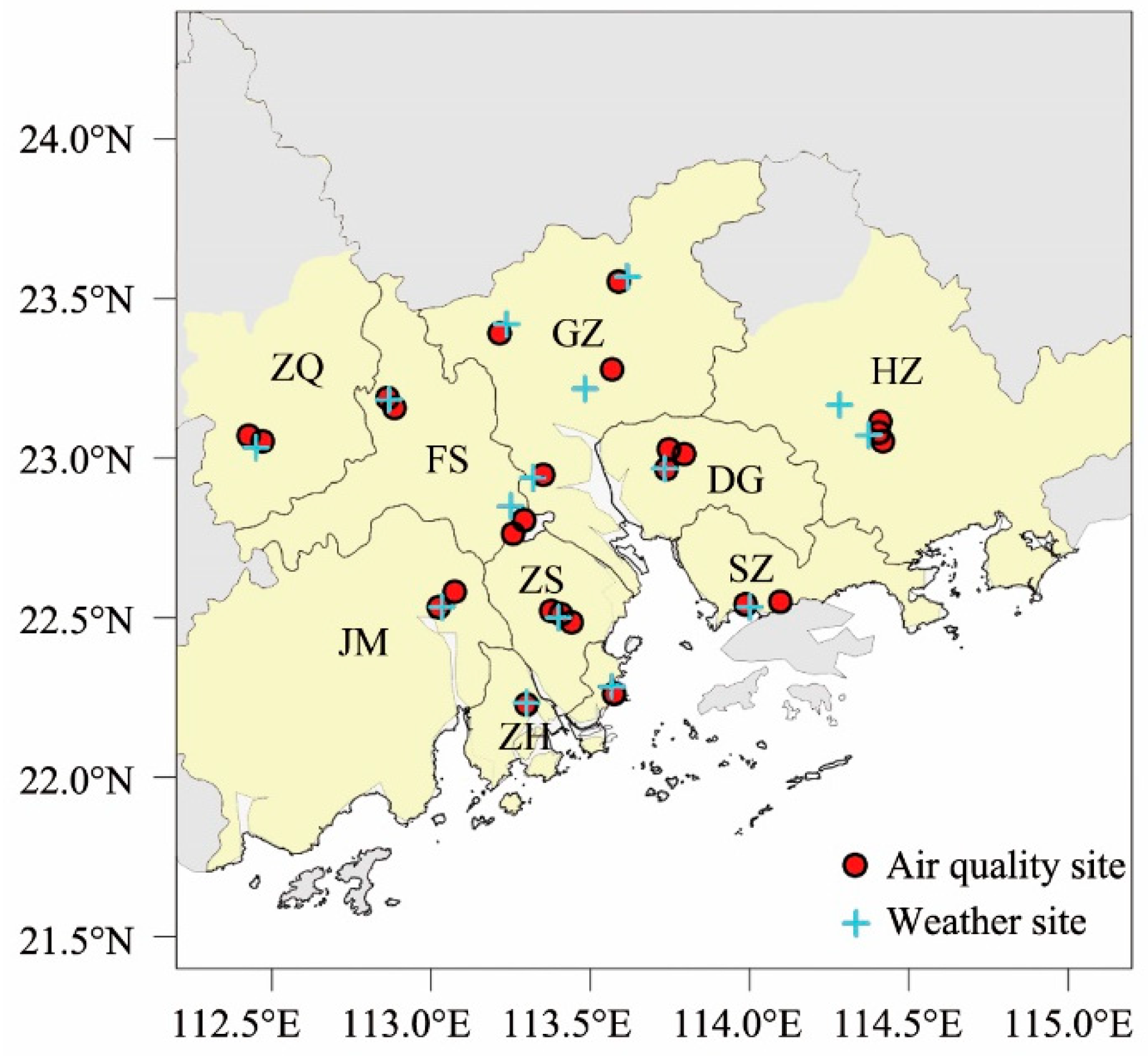
2.1. Observation Data and Case Study

Six-hourly visibility data obtained from the Global Telecommunication System (GTS) [22], hourly near-surface meteorological observation data (wind speed, wind direction, temperature and relative humidity) collected from China Meteorological Administration (CMA) ground-based stations, and reanalysis data obtained from the European Centre for Medium-Range Weather Forecasts Interim Reanalysis (ERA-Interim) [23] at a 0.25° × 0.25° resolution were used to analyze the synoptic situation. To analysis the atmospheric chemistry conditions during this haze event lasting from 14 to 25 January and evaluate the simulation results, we used hourly air quality monitoring data (PM_2.5, PM₁₀, SO₂, NO₂, CO, and O₃) obtained from the Chinese Ministry of Environmental Protection (CMEP) [24].

In this study, the spatial scope of the PRD is shown by the yellow shaded area in Figure 1 and includes GZ, Shenzhen (SZ), ZS, ZH, FS, JM, DG, Huizhou (HZ) (excluding Longmen), and Zhaoqing (ZQ) but not Hong Kong or Macao. Time we mentioned in this study is Beijing time (BJT).

In this case study, a “haze station” was recorded when a station had the visibility below 10 km and the relative humidity lower than 90%, excluding precipitation, blowing snow, blowing sand, sandstorm, floating dust, smoke screen and other obstruction phenomenon to vision [25]. When more than 7 of the 15 surface meteorological observation stations in the PRD were recorded as “haze stations” at any time, a regional haze event occurred [26].

PM_2.5 was the primary atmospheric pollutant in this haze event lasting from 14 to 25 January because its individual air quality index (IAQI) [27] was always higher than that of any other atmospheric chemistry constituents when the air quality index (AQI) [27] was 50 or higher (Figure S1). This event can be divided into three stages according to synoptic conditions (Figure 2) and the change in the regional average PM_2.5 concentration (Figure 3). (1) The slow growth stage from January 15 to 18. The PRD was under the control of northerly winds, and the PM_2.5 concentration changed from less than 50 μg/m³ to over 100 μg/m³, causing regional average visibility to be reduced to below 10 km. The AQI in large cities indicated slight pollution (100 ≤ AQI < 150). (2) The sharp growth stage from 19 to 22 January. The PRD was heavily polluted, and the regional 10-m wind speed was lower than the previous period especially on 20 January when it was less than 1 m/s. The daily AQI in large cities grew rapidly from 19 to 20 January, and was maintained at a high level of up to 150 with the minimum visibility below 5 km on 20 and 21 January. The AQI and PM_2.5 concentration in northern PRD cities such as GZ reached a peak on 21 January, which was one day earlier than that in cities in the southern PRD, such as SZ. (3) The recovery stage from January 23 to 25. The PRD was controlled by southerly winds, and air quality improved in most cities, with AQI values of approximately 100 and PM_2.5 concentrations of approximately 75 μg/m³ (excluding ZQ, which is a city in the northwestern PRD), the second grade standard of the Ambient Air Quality Standard (GB 3095-2012) [28].

From 18 to 19 January, much of southern China was controlled by a high-pressure system (Figure S2), with northerly winds across Hunan, Hubei and even the Yangtze River Delta (YRD) region and reaching the PRD region. This high-pressure system facilitated the long-distance transport of pollutants from north to south. From 08:00 on 19 January to 08:00 on 20 January, the high-pressure system moved eastward over the sea. On 20 January, affected by the transformed high pressure and the surface inverted trough, the surface wind was low. This was conducive to the accumulation of pollutants and aggravated pollution in the PRD. Most of the eastern region of China was re-controlled by the new high-pressure system on 21 January, on which the PRD was at the bottom of the high-pressure system and the northerly wind speed increased. PM_2.5 concentration in the PRD region increased from north to south until noon on 21 January, caused by the upstream pollutants spreading southward along the dominant wind direction. However, it rapidly declined until 23 January. Then, a low-pressure system developed over southwestern China, and clean air mass from the sea that moved toward the PRD alleviated air pollution.

2.2. Model and Simulation Setup

To investigate the effects of pollutant transport on PM_2.5 concentration in the PRD region, three-dimensional simulations with the WRF-Chem model (version 3.9.1) were conducted [29]. This model was developed by the National Center for Atmospheric Research (NCAR), the National Oceanic and Atmospheric Administration, the Air Force Weather Agency (AFWA), the Naval Research Laboratory, the University of Oklahoma, and the Federal Aviation Administration (FAA) [30]. Two nested domains were employed. The parent domain (D01), which is centered at 27.5° N, 113.5° E, has a horizontal resolution of 36 km × 36 km, and the subdomain (D02) has a 12 km × 12 km resolution (Figure 4). 21° N–24° N, 112° E–115° E was defined as the domain of emission source sensitivity experiment (DS). Each domain has 48 vertical layers extending from the surface to the 100-hPa level, of which 21 layers are within 2 km (above ground level (AGL)) to adequately resolve the planetary boundary layer (PBL) structure and local atmospheric circulation under stable weather conditions. All of the model domains use the same parameterization scheme (

Table 1. Physical parameterization schemes used in the simulations.

Parameter	Configurations
Microphysics scheme	Morrison scheme [38]
PBL scheme	MYJ scheme [39]
Cumulus scheme	Grell-Freitas scheme [40]
Land surface scheme	Noah Land Surface Model [41]
Longwave / shortwave radiation scheme	RRTMG scheme [42]
Chemical scheme	RADM2 -MADE/SORGAM [43,44,45]
Photolysis option	Fast-J photolysis [46]

). The simulations were initialized at 08:00 on 16 January 2015, and ran for 217 h until 08:00 on 25 January. The first 40 h were considered as the spin-up period [31,32].

The initial and boundary meteorological conditions were provided by the National Center for Environmental Prediction Global Final Analysis (NCEP-FNL) 6-hourly reanalysis dataset [33] with a horizontal resolution of 1° × 1°. The anthropogenic emissions were set based on monthly Meta-analysis with Interactive eXplanations (MIX) inventory data (2010) [34,35] provided by sector at a 0.25° × 0.25° resolution, including both gaseous species and aerosol species: SO₂, NOx, CO, non-methane volatile organic compounds (NMVOCs), NH₃, PM₁₀, PM_2.5, BC, OC and CO₂. In addition, biological emissions were calculated online by the Model of Emissions of Gases and Aerosols from Nature (MEGAN) [36]. The initial and boundary chemical conditions were obtained from the global output of the Model for Ozone and Related chemical Tracers (MOZART) [37].

To explore the impact of emissions transport on the PM_2.5 concentration in the PRD, three experiments were conducted using the emission zero-out method [2,47,48] as follows: (1) Control experiment (CTL), with all emissions; (2) Local experiment (LC), with only emissions in the DS region (21° N–24° N, 112° E–115° E), to indicate the impact of local emissions in the PRD region; (3) Transport experiment (TR), excluding emissions in the DS region, to indicate the impact of cross-regional transport from outside the PRD region. According to Grewe et al. [49], the emission zero-out method tends to underestimate the actual contribution of target emissions to secondary pollutants, mainly caused by nonlinearity in atmospheric chemistry which could be calculated by (TR+LC)-CTL [50]. It will be discussed in Section 3.3.

2.3. Calculation of the Trans-Regional Transport of Pollutants

A simplified boundary model is established, as shown in Figure 5 and

Table 2. Information on the simplified boundary of the PRD region.

Name	Starting Location	Ending Location	Length (km)	Average Elevation (m)	${\mathit{\theta }}_{\mathit{n}}(°)$
North (AB)	113.10° E, 23.78° N	114.38° E, 23.78° N	136	234	0
East (BC)	114.38° E, 23.78° N	115.28° E, 22.88° N	136	212	45
Southeast (CD)	115.28° E, 22.88° N	112.19° E, 21.64° N	347	22	22.5
West (DE)	112.19° E, 21.64° N	112.19° E, 22.88° N	136	145	90
Northwest (EA)	112.19° E, 22.88° N	113.10° E, 23.78° N	136	95	45

Note: ${\theta }_n$ is the minimum angle between the boundary and horizontal.

. The cross-regional transport intensity of PM_2.5 in the unit grid at different layers under each boundary condition is calculated at each time. The “closed line method”, proposed by Yang et al. [51], is used to calculate the concentration transport flux intensity of the region bounded by the simplified boundary [50].

It is assumed that the concentration of pollutants $P$ at grid point (at time $t$) $(t,k,j,i)$ ($k$: layer; $j$: meridional location; $i$: zonal location) is $P_{t,k,j,i}$. Taking boundary AB as an example, boundary vectors and their corresponding normal vectors are defined as ${\overrightarrow{I}}_n$ (pointing from A to B; $n$: boundary;) and ${\overrightarrow{N}}_n$ (perpendicular to AB and pointing to the interior of the PRD), respectively. $W_{n,t,k,j,i}$ is the projection length of the wind vector $\overrightarrow{U}(U_{t,k,j,i},V_{t,k,j,i})$ onto ${\overrightarrow{N}}_n$ at any point $(t,k,j,i)$ on the boundary AB. A positive value of $W_{n,t,k,j,i}$ represents the cross-regional input of pollutants into the PRD, while a negative value represents the cross-regional output outside of the PRD. $pn$ is the number of grids along the boundary $n$ at each layer, and $kn$ is the number of layer.

The projection length of the wind vector $\overrightarrow{U}$can be calculated as follows:

$$W_{n,t,k,j,i}=V_{t,k,j,i}\cdot \cos {\theta }_n+U_{t,k,j,i}\cdot \sin {\theta }_n,$$

(1)

The average transport flux intensity $F_{n,t,k}$ at time $t$ and level $k$ through boundary n can be calculated by the discrete summation method,

$$F_{n,t,k}=\frac{1}{pn}{\displaystyle \sum _{(i=1,j=1)}^{(pn,pn)}{P}_{t,k,j,i}\cdot W_{n,t,k,j,i}},$$

(2)

$M_{n,t}$ is used to represent the average transport flux intensity across boundary n at time $t$ at a level below 3 km,

$$M_{n,t}=\frac{1}{kn}{\displaystyle \sum _{k=1}^{kn}{F}_{n,t,k}}=\frac{1}{pn\cdot kn}{\displaystyle \sum _{k=1}^{kn}{\displaystyle \sum _{(i=1,j=1)}^{(pn,pn)}{P}_{t,k,j,i}\cdot W_{n,t,k,j,i}}},$$

(3)

3. Results

In this section, the CTL simulation results are evaluated by observations at first; then, the distribution of the PM_2.5 concentration simulated by the three experiments is described. Finally, the effects of extra-regional transport and cross-regional transport of PM_2.5 are discussed.

3.1. Evaluation of the Simulation Results

The 10-m wind, 2-m temperature (T2), 2-m relative humidity (RH2), and near-surface PM_2.5 concentration from 18 to 24 January simulated by the CTL experiment were compared based on the observation data from 15 stations in the PRD (Figure 6). In terms of T2 and RH2, good agreement was found between the CTL simulation and observations, with high correlation coefficients (R) of 0.96 and 0.90 (p < 0.01), respectively. The model tended to overestimate the speed of the 10-m wind, but the simulated wind direction was basically the same as the observed wind direction (mainly northerly winds for both). With respect to regional PM_2.5 concentration, the model could simulate the variation characteristics, with an R value of 0.35 (p < 0.01), and root mean square error (RMSE) of 32.90 μg/m³, not as good as meteorological elements but still within double errors (Figure S3). Besides, it tended to underestimate most of the time, especially during the stage of weak wind and shear (12:00–20:00, 20 January) and the stage in which the northerly surface wind speed increased sharply (12:00–24:00, 21 January). The comparison of observations and simulation results among cities (Figure 7,

Table 3. Statistics of the hourly simulation results of the PM_2.5 concentration in cities in the PRD.

Parameter 1	PRD	GZ	SZ	ZH	FS	ZS	JM	DG	HZ	ZQ
MO (μg/m3)	74.6	82.9	62.2	73.5	78.0	65.9	84.1	84.1	54.3	81.9
MC (μg/m3)	49.7	67.1	41.5	49.4	70.3	49.6	63.3	65.3	53.2	54.8
MB (μg/m3)	−24.9	−15.8	−20.7	−24.1	−7.6	−16.3	−20.8	−18.7	−1.1	−27.1
NMB (%)	−33.4	−19.0	−33.3	−32.8	−9.8	−24.7	−24.7	−22.3	−2.1	−33.1
NME (%)	41.2	27.2	38.0	33.8	21.9	35.4	29.3	29.1	34.4	35.3
RMSE (μg/m3)	32.9	29.3	33.21	29.1	23.1	33.1	32.3	30.3	23.1	34.7

¹ MO: Mean of the OBS. MC: Mean of the CTL. MB: Mean bias between the OBS and CTL. NMB: Normalized mean bias. NME: Normalized mean error. RMSE: Root mean square error.

) showed that the R values of GZ, FS and DG were 0.67, 0.66, and 0.66, with normalized mean biases (NMBs) of 19.01%, 9.80%, and 22.28%, respectively. The increase in PM_2.5 concentration on 20 and 21 January in northern cities was also reflected by the simulation. For SZ and ZS (the cities in the southern PRD), the time at which the simulated concentration reached its peak was 6 to 13 h earlier than that of the observation, which was caused by the earlier increase in northerly wind speed. Northerly winds brought upstream pollutants downstream and made the PM_2.5 concentration increase in advance of downstream cities.

Overall, the model could simulate the haze event and be appropriate for studying the impacts of PM_2.5 transport on haze events in the PRD with reasonable deviation. Errors between observation and simulation are associated with several aspects including the selection of different physical parameterization schemes, differences between the initial fields and observations and systematic errors due to the set-up of model. For chemistry elements such as PM_2.5, simulated results are also affected by meteorological elements (such as wind speed, temperature, and PBL height (PBLH)), emission inventories and chemical mechanisms [8,52,53]. Therefore, whether the model systematically underestimated the PM_2.5 concentration in the PRD region needs to be further investigated through other cases and by improving accuracy of emission inventories, comparing different combinations of physical parameters selections.

3.2. Distribution of PM_2.5 near the Surface

Simulated near-surface PM_2.5 concentrations, wind fields and sea level pressure during the pollution process are shown in Figure 8. Highly polluted regions caused by PM_2.5 were mainly in Sichuan Province and the northern part of the YRD. Located at the southern edge of the surface high-pressure system on 19 and 21 January, the PRD was controlled by prevailing northerly winds, which brought PM_2.5 downstream from those polluted regions, causing an increase in daily concentration in the PRD. On 20 January, controlled by the surface reverse trough, the isobaric lines over the PRD were spaced out, and the airflow was stagnant, which was not conducive to the horizontal diffusion of pollutants, causing the PM_2.5 concentration in the central PRD to sharply increase from 75 μg/m³ to 115 μg/m³. Meanwhile, located between the surface reverse trough (west) and surface high-pressure system (east), PM_2.5 was pushed northwards by southerly winds and accumulated in the northern YRD, where the PM_2.5 concentration exceeded 160 μg/m³. From 23 January, the center of the high-pressure system moved away from the mainland, and the prevailing southerly winds controlled the PRD and purified the region. Meanwhile, pollutants in the YRD could still travel along the southeastern coast toward the PRD under a northeasterly wind.

3.3. Extra-Regional and Intra-Regional Transport of PM_2.5

To further explore the impact of extra-regional transport on PM_2.5 concentration in the PRD during the haze event quantitatively, the emission zero-out experiments were designed as described in Section 2.2.

Firstly, contribution of nonlinear response were calculated in different scenarios (Figure 9,

Table 4. Average concentration and contribution of PM_2.5 in PRD for different scenarios.

	CTL	TR	LC	(TR + LC) − CTL
Concentration (μg/m3)	58.96	22.85	19.61	−16.50
Contribution (%)	100	38.75	33.27	−27.98

). It was found that when considering effects of nonlinear response, and average PM_2.5 concentration for transport was 22.85 to 39.35 μg/m³ (CTL-LC) with a contribution of 38.75% to 66.73 %. Besides, higher effects of nonlinearity mostly occurred at time when 10-m wind at a low wind speed (close to zero), or wind direction shifted from northerly to southerly (vice versa). In this case, nonlinear response devoted almost as much as extra-regional transport and local emission did, and further research were in need to find the reasons. This study mainly focused on the process of transport and its effects without considering nonlinear response. Therefore, the contributions of PM_2.5 to the PRD caused by extra-regional transport ($C_{TR}$) and intra-regional transport ($C_{LC}$) were defined by the simulated results of the TR and LC experiments, respectively. The contribution rate of extra-regional transport was expressed as $G=100\%\times C_{TR}/(C_{TR}+C_{LC})$.

The distributions of the near-surface PM_2.5 concentration in the three simulation experiments were compared in Figure 10. Without considering nonlinear response, extra-regional transport of PM_2.5 had an important impact on the PRD, particularly for cities along the upstream edge, with daily concentrations of 10 to 50 μg/m³. Notably, even under a weak circulation background, 10 to 30 μg/m³ of PM_2.5 was still caused by extra-regional transport. Local emissions mainly affected the Pearl River Estuary, and the maximum daily contribution was 70 to 90 μg/m³. In addition, the intra-regional transport of pollutants was also important to downwind areas, contributing at least 10 to 30 μg/m³ daily.

Quantitative analysis showed that the average contribution of extra-regional transport to the hourly PM_2.5 concentration in the PRD was 22.85 μg/m³, where the average contribution rate was 56.48% (Figure 11). Extra-regional transport had great significance in GZ, SZ, and JM, three cities located in different regions of the PRD. The wind speed near the surface was higher from 12:00 to 20:00 on 21 January and 08:00 to 20:00 on 23 January; the average hourly concentration of PM_2.5 contributed by extra-regional transport to these three cities was 21.16 to 37.27 μg/m³, and the average contribution rate was 52.42% to 93.12%; the variation trends of extra-regional transport contribution in three cities were similar, excluding a higher concentration contribution in coastal city SZ and JM than that in the northern city GZ, when controlled by southerly winds from 00:00 on 23 January to 00:00 on 25 January. However, total surface PM_2.5 concentration in SZ still decreased and maintained at a low level around 50 μg/m³ during 23 to 24 January, much less than that in 21 to 22 January (Figure 7b). The transport of marine aerosols and pollutant composition should be taken into consideration for further analysis in the future. SZ and JM were likely to be affected by pollutants coming from Hong Kong and the YRD region under the dominant wind (Figure 8d, Figure 9h).

Taking SZ (22.55° N, 114.10° E) as an example to study the relationship between the influence of extra-regional transport on the variation in PM_2.5 concentration and turbulent kinetic energy (TKE) (Figure 12), the influence of extra-regional transport on the PM_2.5 concentration was found to be mainly below 1 km, with a maximum concentration contribution of 50 to 60 μg/m³, especially at night to early morning. The TKE in the boundary layer was weak during this period, which was not conducive to the vertical diffusion of pollutants and conducive to enhancing the effect of extra-regional transport on the PM_2.5 concentration. From noon on 21 January to noon on 22 January, affected by the northerly wind, the main transport channel of extra-regional pollutants was up to an altitude of 2.5 km. From 23 to 24 January, affected by the southerly wind, the transport channel reached 1.5 km but was concentrated below 0.5 km, with a contribution of 20 to 50 μg/m³. This result indicated that southerly wind also had an extra-regional transport impact on PM_2.5. The smaller the vertical variation in the horizontal wind direction and the greater the wind speed, the more favorable the extra-regional transport of PM_2.5 was.

The process of the long-distance transport of PM_2.5 was further explored through the latitude-height profile (Figure 13), which is still based on the city of SZ (22.55° N, 114.10° E).

From 20 to 21 January, with the eastward movement of the surface high pressure, the northerly wind below 3 km was enhanced in southern China, causing the transport of PM_2.5 southward across the Nanling Mountains to affect the PRD region. From 23 January on, meridional wind below 3 km shifted to southerly, and the transport was much weaker than that under a northerly wind. On the one hand, the southerly wind was truly able to bring the polluted air mass from the upwind region across the ocean to the PRD. However, the meridional wind was reduced, which was not sufficient to promote the transport of polluted air masses to pass over the Nanling Mountains and go north. On the other hand, from 23 January on, PRD was controlled by downward flow coming from the south side, inhibiting the vertical diffusion of pollutants and enhancing the pollution. But the mixing below the PBL was much greater than that in 20 January, so the surface concentration could maintain at around 50 μg/m³.

3.4. Cross-Regional Transport of PM_2.5

Considering the terrain of the PRD, which is backed by the mainland and facing the sea, a simplified boundary model was established, as shown in Figure 5. The temporal and spatial variations in the transport intensity of PM_2.5 across different boundaries are shown in Figure 14.

The main path height of PM_2.5 was from 0.1 to 0.7 km (AGL, below). The net flux of the PM_2.5 concentration before 12:00 on 22 January was positive, showing that extra-regional transport during this period promoted the increase in PM_2.5 concentration. The main input paths are from the north boundary, the northeastern boundary and the northwestern boundary, and the maximum transport intensity was 0.84 × 10³ μg·m⁻²·s⁻¹, which appeared at approximately 1.2 km at 18:00 on 21 January; the maximum total flux intensity was 9.68 × 10³ μg·m⁻²·s⁻¹below 3 km. Specifically, affected by the low wind speed on 20 January, the average transport flux intensity at each boundary below 3 km was so small that it was close to zero. In other words, the increase in PM_2.5 was mainly related to local weather conditions. The main path height increased to 2.5 km, which was influenced by the prevailing northerly wind below 3 km, greatly increasing the transport rate of polluted air masses moving into the PRD, and leading to intensified pollution. During 23 to 24 January, due to the southerly wind bringing relatively clean air mass, the net flux of PM_2.5 into the PRD was negative and pollution was alleviated excluding coastal region in the southern PRD. Composition analysis and Potential source contribution function (PSCF) are demanded to further study whether the southeast source is from the ocean or Hong Kong and its influencing mechanism.”

4. Conclusions and Discussion

In this study, the impact of the cross-regional transport of pollutants on a haze event in the PRD region from 14 to 25 January in 2015 was studied by observation analysis and numerical simulation.

(1) According to the observations, PM_2.5 was the primary pollutant in this haze event. PM_2.5 increased one day earlier in the northern PRD than that in the southern PRD under the control of a prevailing northerly wind due to the combined action of local emissions and trans-boundary transport.

(2) The haze event was simulated well by the CTL simulation experiment. During the first stage of this haze event, it was found that the PRD region was located at the bottom of the surface high-pressure and controlled by the northerly wind, a synoptic pattern that was conducive to the transport and diffusion of PM_2.5 from the upstream area. The cross-regional transport resulted in the rapid increase in the PM_2.5 concentration in the northern PRD, which occurred one day earlier than the increase in the southern PRD. In the second stage of the haze event, the PRD was located under the weak surface trough system, and the air flow was stagnant and counteracted the horizontal diffusion of pollutants, which resulted in a rapid increase in the PM_2.5 concentration in the PRD and the intensification of regional pollution. During the third stage of this haze event, the PRD was located under the saddle area between the high-pressure (east) and low-pressure (west) systems. The surface wind turned from northerly to southerly, and the relatively clean air mass caused the alleviation of pollution in the PRD. In addition, the upwind region in the PRD was more susceptible to PM_2.5 trans-boundary transport than the central region, where local emissions were more important to pollution. In addition, intra-regional transport should not be ignored during haze events. Without considering nonlinear response, the extra-regional transport of PM_2.5 could contribute approximately 22.9 μg/m³ to the hourly concentration of PM_2.5 in the PRD on average, which accounted for 56.5% of the average contribution rate. The transport was mainly located in the boundary layer, which was approximately 1 km high, and could increase up to 1.5 km when the PRD was controlled by a southerly wind, but transport was mainly concentrated below 0.5 km. When controlled by a northerly wind, the transport height could reach 2.5 km. The more uniform the horizontal wind direction and the higher the wind speed, the more favorable the extra-regional long-distance transport of PM_2.5 was.

(3) When the PRD was influenced by a northerly wind, the main trans-boundary transport of PM_2.5 occurred mainly at altitudes of 0.1 to 0.7 km. The maximum total transport flux intensity below 3 km was 9.7 × 10³ μg·m⁻²·s⁻¹, with a maximum transport intensity of 0.84 × 10³ μg·m⁻²·s⁻¹ that appeared at approximately 1.2 km at 18:00 on 21 January. When the PRD was controlled by a southerly wind, pollution in coastal cities was intensified by the input of a marine air mass. However, pollution was mitigated in this case when taking the PRD region as a whole. During the period of low wind speed, the average transport flux intensity below 3 km was too small, and the increase in PM_2.5 was mainly related to local meteorological conditions.

This study explained the characteristics and processes of PM_2.5 cross-boundary transport, to some extent, through observational analysis and numerical simulations obtained from the WRF-Chem model. Model simulations could reproduce the main characteristics of the haze process. Nonetheless, there were some uncertainties due to numerical simulation error, nonlinear response to chemical reactions among pollutants, and emissions not being sufficiently precise, which could be improved through better experimental design by adjusting and optimizing the parameterization scheme. Beside of pollutants transport, the high temperature and high environmental relative humidity were also conducive to aerosol aging and growth, resulting in the further aggravation of pollution downstream. However, limited by data obtaining, this study was in lack of vertical observation and analysis of aerosol compositions, which could help us to understand the reasons why PM_2.5 concentration maintained at around 50 to 70 μg/m³ (a slightly polluted level) under the control of relatively clean air mass brought by southerly winds. This work will be improved and keep on moving further.

References

1. Wu, D.; Bi, X.; Deng, X.; Li, F.; Tan, H.; Liao, G.; Huang, J. Effect of atmospheric haze on the deterioration of visibility over the Pearl River Delta. Acta Meteorol. Sin. 2006, 64, 510–517. (In Chinese) [Google Scholar]
2. Lyu, W.; Li, J.; Wang, X.; Zhang, Y. Numerical modeling on the impact of long-range transport of air pollutants on the regional air quality in the Pearl. Acta Sci. Circumstantiae 2015, 35, 30–41. (In Chinese) [Google Scholar] [CrossRef]
3. Tao, Y.; Zhong, L.; Huang, X.; Lu, S.E.; Li, Y.; Dai, L.; Zhang, Y.; Zhu, T.; Huang, W. Acute mortality effects of carbon monoxide in the Pearl River Delta of China. Sci. Total Environ. 2011, 410, 34–40. [Google Scholar] [CrossRef] [PubMed]
4. Wu, D.; Tie, X.; Li, C.; Ying, Z.; Lau, K.H.; Huang, J.; Deng, X.; Bi, X. An extremely low visibility event over the Guangzhou region: A case study. Atmos. Environ. 2005, 39, 6568–6577. [Google Scholar] [CrossRef]
5. Sun, Y.; Chen, C.; Zhang, Y.; Xu, W.; Zhou, L.; Cheng, X.; Zheng, H.; Ji, D.; Li, J.; Tang, X. Rapid formation and evolution of an extreme haze episode in Northern China during winter 2015. Sci. Rep. 2016, 6, 27151. [Google Scholar] [CrossRef]
6. Yang, Y.; Liu, X.; Yu, Q.; Wang, J.; An, J.; Zhang, Y.; Fang, Z. Formation mechanism of continuous extreme haze episodes in the megacity Beijing, China, in January 2013. Atmos. Res. 2015, 155, 192–203. [Google Scholar] [CrossRef]
7. Chen, H.; Wang, Z.; Wu, Q.; Wang, W. Source analysis of Guangzhou air pollutants by numerical simulation in the Asian Games Period. Acta Sci. Circumstantiae 2010, 30, 2145–2153. (In Chinese) [Google Scholar] [CrossRef]
8. Guo, J.; Lou, M.; Miao, Y.; Wang, Y.; Zeng, Z.; Liu, H.; He, J.; Xu, H.; Wang, F.; Min, M. Trans-Pacific transport of dust aerosols from East Asia: Insights gained from multiple observations and modeling. Environ. Pollut. 2017, 230, 1030–1039. [Google Scholar] [CrossRef]
9. Huang, J.; Minnis, P.; Chen, B.; Huang, Z.W.; Ayers, J.K. Long-range transport and vertical structure of Asian dust from CALIPSO and surface measurements during PACDEX. J. Geophys. Res. Atmos. 2008, 113. [Google Scholar] [CrossRef]
10. Miao, Y.; Guo, J.; Liu, S.; Liu, H.; Zhang, G.; Yan, Y.; Jing, H. Relay transport of aerosols to Beijing-Tianjin-Hebei region by multi-scale atmospheric circulations. Atmos. Environ. 2017, 165, 35–45. [Google Scholar] [CrossRef]
11. Wang, W.; Chen, H.S.; Wu, Q.; Wei, L.; Wang, Z.; Li, C.; Chen, D.; Jiang, Z.; Wu, W. Numerical study of PM2.5 regional transport over Pearl River Delta during a winter heavy haze event. Acta Sci. Circumstantiae 2016, 36, 2741–2751. (In Chinese) [Google Scholar]
12. Wang, Z.F.; Jie, L.; Wang, Z.; Yang, W.Y.; Tang, X.; Baozhu, G.E.; Yan, P.Z.; Zhu, L.L.; Chen, X.S.; Chen, H.S. Modeling study of regional severe hazes over mid-eastern China in January 2013 and its implications on pollution prevention and control. Sci. China Earth Sci. 2014, 57, 3–13. [Google Scholar] [CrossRef]
13. Fan, S.; Wang, A.; Fan, Q.; Liu, J.; Wang, B. Atmospheric boundary layer features of Pearl River Delta and its conception model. China Environ. Sci. 2006, 26, 4–6. [Google Scholar]
14. Wu, D.; Liao, B.; Chen, H.; Wu, S. Advances in studies of haze weather over Pearl River Delta. Clim. Environ. Res. 2014, 19, 248–264. [Google Scholar] [CrossRef]
15. Wu, D.; Liao, G.; Deng, X.; Bi, X.; Tan, H.; Li, F.; Jiang, C.; Xia, D.; Fan, S. Transport condition of surface layer under haze weather over the Pearl River Delta. J. Appl. Meteorol. 2008, 19, 1–9. [Google Scholar]
16. Dongwei, W.U.; Fung, J.C.H.; Yao, T.; Lau, A.K.H. A study of control policy in the Pearl River Delta region by using the particulate matter source apportionment method. Atmos. Environ. 2013, 76, 147–161. [Google Scholar] [CrossRef]
17. Xue, W.; Fu, F.; Wang, J.; Tang, G.; Lei, Y.; Yang, J.; Wang, Y. Numerical study on the characteristics of regional transport of PM2.5 in China. China Environ. Sci. 2014, 34, 1361–1368. (In Chinese) [Google Scholar]
18. Xue, W.; Tang, X.; Lei, Y.; Wang, J.; Xu, Y. Impacts of ammonia emission on PM2.5 pollution in China. China Environ. Sci. 2016, 36, 3531–3539. (In Chinese) [Google Scholar]
19. Kasten, F. Falling speed of aerosol particles. J. Appl. Meteorol. 1968, 7, 4. [Google Scholar] [CrossRef]
20. Wang, S.; Zhang, Y.; Zhong, L.; Li, J.; Yu, Q. Interaction of urban air pollution among cities in Zhujiang Delta. China Environ. Sci. 2005, 25, 133–137. (In Chinese) [Google Scholar]
21. Hu, X.; Li, Y.; Li, J.; Wang, X.; Zhang, Y. Interaction of ambient PM10 among the cities over the Pearl River Delta. Acta Sci. Nat. Univ. Pekin. 2011, 47, 519–524. (In Chinese) [Google Scholar] [CrossRef]
22. GTS dataset Archive. Available online: http://222.195.136.24/forecast.html (accessed on 30 May 2017).
23. ERA-Interim Daily Dataset Archive. Available online: https://apps.ecmwf.int/datasets/data/interim-full-daily/levtype=sfc/ (accessed on 30 May 2017).
24. CMEP Hourly Air Quality Monitoring Dataset Archive. Available online: http://106.37.208.233:20035/ (accessed on 30 May 2017). (In Chinese).
25. Guangzhou Institute of Tropical and Marine Meteorology, C.M.A. Observation and Forecasting Levels of Haze. QX: 2010; Vol. QX/T 113-2010, p 8p:A4. Available online: http://www.cma.gov.cn/root7/auto13139/201612/P020161223252938063210.pdf (accessed on 18 April 2019). (In Chinese)
26. Chen, H.; Wang, H. Haze Days in North China and the Associated Atmospheric Circulations Based on Daily Visibility Data from 1960 to 2012. J. Geophys. Res. Atmos. 2015, 120, 5895–5909. [Google Scholar] [CrossRef]
27. Centre, C.N.E.M.; Sciences, C.R.A.O.E.; Center, D.E.M.; Center, S.E.M.; Center, S.E.M.; Center, J.E.M.; Center, H.E.M.; Center, C.E.M. Technical Regulation on Ambient Air Quality Index(on Trial). CN-HJ: 2012; Vol. HJ 633-2012, p 12P.;A14. Available online: http://kjs.mee.gov.cn/hjbhbz/bzwb/jcffbz/201309/W020131105548549111863.pdf (accessed on 18 April 2019). (In Chinese)
28. Sciences, C.R.A.o.E.; Centre, C.N.E.M. Ambient Air Quality Standard. PRC National Standard: 2012; Vol. GB 3095-2012, p 12p:A14. Available online: http://kjs.mee.gov.cn/hjbhbz/bzwb/dqhjbh/dqhjzlbz/201203/W020120410330232398521.pdf (accessed on 18 April 2019). (In Chinese)
29. Grell, G.A.; Schmitz, P.R.; Mckeen, S.A.; Frost, G.; Skamarock, W.C.; Eder, B. Fully coupled “online” chemistry within the WRF model. Atmos. Environ. 2005, 39, 6957–6975. [Google Scholar] [CrossRef]
30. Homepage of WRF-Chem. Available online: https://ruc.noaa.gov/wrf/wrf-chem/ (accessed on 18 April 2019).
31. Kleczek, M.A.; Steeneveld, G.J.; Holtslag, A.A.M. Evaluation of the Weather Research and Forecasting Mesoscale Model for GABLS3: Impact of Boundary-Layer Schemes, Boundary Conditions and Spin-Up. Bound. Lay. Meteorol. 2014, 152, 213–243. [Google Scholar] [CrossRef]
32. Miao, Y.; Liu, S.; Zheng, Y.; Wang, S.; Chen, B.; Zheng, H.; Zhao, J. Numerical study of the effects of local atmospheric circulations on a pollution event over Beijing–Tianjin–Hebei, China. J. Environ. Sci. 2015, 30, 9–20. [Google Scholar] [CrossRef]
33. NCEP-FNL Reanalysis Dataset Archive. Available online: https://rda.ucar.edu/datasets/ds083.2/ (accessed on 30 May 2017).
34. Li, M.; Zhang, Q.; Kurokawa, J.; Woo, J.H.; He, K.; Lu, Z.; Ohara, T.; Song, Y.; Streets, D.G.; Carmichael, G.R. MIX: A mosaic Asian anthropogenic emission inventory under the international collaboration framework of the MICS-Asia and HTAP. Atmos. Chem. Phys. 2017, 17, 935–963. [Google Scholar] [CrossRef]
35. MIX Asian Emission Inventory. Available online: http://www.meicmodel.org/dataset-mix.html (accessed on 30 May 2017).
36. Guenther, A.; Karl, T.; Harley, P.; Wiedinmyer, C.; Palmer, P.I.; Geron, C. Estimates of global terrestrial isoprene emissions using MEGAN (Model of Emissions of Gases and Aerosols from Nature). Atmos. Chem. Phys. 2006, 6, 3181–3210. [Google Scholar] [CrossRef]
37. MOZART dataset download Archive. Available online: http://www.acom.ucar.edu/wrf-chem/mozart.shtml (accessed on 30 May 2017).
38. Morrison, H.; Thompson, G.; Tatarskii, V. Impact of Cloud Microphysics on the Development of Trailing Stratiform Precipitation in a Simulated Squall Line: Comparison of One- and Two-Moment Schemes. Mon. Wea. Rev. 2009, 137, 991–1007. [Google Scholar] [CrossRef]
39. Janjić, Z.I. The Step-Mountain Eta Coordinate Model: Further Developments of the Convection, Viscous Sublayer, and Turbulence Closure Schemes. Mon. Weather Rev. 1994, 122, 927. [Google Scholar] [CrossRef]
40. Arakawa, A. The Cumulus Parameterization Problem: Past, Present, and Future. J. Climate 2004, 17, 2493–2525. [Google Scholar] [CrossRef]
41. Chen, F.; Dudhia, J. Coupling an Advanced Land Surface–Hydrology Model with the Penn State–NCAR MM5 Modeling System. Part I: Model Implementation and Sensitivity. Mon. Weather Rev. 2001, 129, 569–585. [Google Scholar] [CrossRef]
42. Iacono, M.J.; Delamere, J.S.; Mlawer, E.J.; Shephard, M.W.; Clough, S.A.; Collins, W.D. Radiative forcing by long-lived greenhouse gases: Calculations with the AER radiative transfer models. J. Geophys. Res. Atmos. 2008, 113. [Google Scholar] [CrossRef]
43. Ackermann, I.J.; Hass, H.; Memmesheimer, M.; Ebel, A.; Binkowski, F.S.; Shankar, U. Modal aerosol dynamics model for Europe : Development and first applications. Atmos. Environ. 1998, 32, 2981–2999. [Google Scholar] [CrossRef]
44. Schell, B.; Ackermann, I.J.; Hass, H.; Binkowski, F.S.; Ebel, A. Modeling the formation of secondary organic aerosol within a comprehensive air quality model system. J. Geophys. Res. Atmos. 2001, 106, 28275–28293. [Google Scholar] [CrossRef]
45. Stockwell, W.R.; Middleton, P.; Chang, J.S.; Tang, X. The second generation regional acid deposition model chemical mechanism for regional air quality modeling. J. Geophys. Res. Atmos. 1990, 95, 16343–16367. [Google Scholar] [CrossRef]
46. Wild, O.; Zhu, X.; Prather, M.J. Fast-J: Accurate Simulation of In- and Below-Cloud Photolysis in Tropospheric Chemical Models. J. Atmos. Chem. 2000, 37, 245–282. [Google Scholar] [CrossRef]
47. Kwok, R.H.F.; Fung, J.C.H.; Lau, A.K.H.; Fu, J.S. Numerical study on seasonal variations of gaseous pollutants and particulate matters in Hong Kong/Pearl River Delta Region. J. Geophys. Res. 2010, 115. [Google Scholar] [CrossRef]
48. Zhang, L.; Wang, T.; Lyu, M.; Zhang, Q. On the severe haze in Beijing during January 2013: Unraveling the effects of meteorological anomalies with WRF-Chem. Atmos. Environ. 2015, 104, 11–21. [Google Scholar] [CrossRef]
49. Grewe, V. Technical Note: A Diagnostic for Ozone Contributions of Various NOx Emissions in Multi-Decadal Chemistry-Climate Model Simulations. Atmos. Chem. Phys. 2004, 4, 729–736. [Google Scholar] [CrossRef]
50. Wang, L.; Hao, J.; He, K.; Wang, S.; Li, J.; Zhang, Q.; Streets, D.G.; Fu, J.S.; Jang, C.J.; Hideto, T.; et al. A Modeling Study of Coarse Particulate Matter Pollution in Beijing: Regional Source Contributions and Control Implications for the 2008 Summer Olympics. J. Air Waste Manag. Assoc. 2008, 58, 14. [Google Scholar] [CrossRef]
51. Yang, L.; Wang, X.; Chen, Q. New method for investigating regional interactions of air pollutants. Acta Sci. Circumstantiae 2012, 32, 528–536. (In Chinese) [Google Scholar]
52. Balzarini, A.; Honzak, L.; Pirovano, G.; Riva, G.M.; Zabkar, R. WRF-Chem Model Sensitivity Analysis to Chemical Mechanism Choice. 2014. Available online: https://link.springer.com/chapter/10.1007/978-3-319-04379-1_92 (accessed on 22 March 2019).
53. Ritter, M.; Müller, M.D.; Jorba, O.; Parlow, E.; Liu, L.J.S. Impact of chemical and meteorological boundary and initial conditions on air quality modeling: WRF-Chem sensitivity evaluation for a European domain. Meteorol. Atmos. Phys. 2013, 119, 59–70. [Google Scholar] [CrossRef]
Figure 1. Spatial distribution of the meteorological observation sites and atmospheric environment monitoring sites in the Pearl River Delta (PRD) (meteorological observation sites: Weather site, Blue “+”; atmospheric environment monitoring sites: Air quality site, Red “●”).
Atmosphere 10 00237 g001
Figure 2. Time series of the (a) number of haze stations (colored bar; unit: number) with regional average visibility (solid line with “△” on it; unit: km) at time 02:00 (“02”), 08:00 (“08”), 14:00 (“14”), and 20:00 (“20”), (b) regional average 10-m wind, and (c) daily air quality index (AQI) of some cities in the PRD from 14 to 25 January 2015.
Atmosphere 10 00237 g002
Figure 3. Hourly concentration of fine particulate matter (PM2.5) in some cities in the PRD from 14 to 25 January 2015. (a) Guangzhou (GZ), Foshan (FS), Dongguan (DG), and Zhaoqing (ZQ); (b) Shenzhen (SZ), Zhuhai (ZH), and Zhongshan (ZS); (c) Jiangmen (JM) and Huizhou (HZ).
Atmosphere 10 00237 g003
Figure 4. The two nested domains and spatial distribution of PM2.5 emissions (shading; unit: μg∙m−2∙s−1). The area enclosed by the dotted line is the DS region.
Atmosphere 10 00237 g004
Figure 5. (a) Simplified boundary (black solid line) of the PRD region and (b) schematic diagram of the trans-boundary transport of pollutants.
Atmosphere 10 00237 g005
Figure 6. Time series of the simulation results of the control experiment (CTL) and observations (OBS). (a) 10-m wind; (b) 2-m air temperature (T2); (c) 2-m relative humidity (RH2).
Atmosphere 10 00237 g006
Figure 7. Time series of the hourly PM2.5 concentration in cities in the PRD. From (a) to (i): GZ, SZ, ZH, FS, ZS, JM, DG, HZ, and ZQ, respectively. OBS values (black solid points, “•”), simulated values (CTL, solid red line, “-”), and deviation value (bias, cyan, “▃”).
Atmosphere 10 00237 g007
Figure 8. The simulation results of the daily average near-surface PM2.5 concentration (shaded; unit: μg/m3), 10-m wind field (blue vector; unit: m/s) and sea level pressure (black contour; unit: hPa). From (a) to (d) are 19, 20, 21, and 23 January, respectively (the solid purple box refers to the emissions control region).
Atmosphere 10 00237 g008
Figure 9. Time series of regional average PM2.5 (a) concentration, (b) contribution rate, and (c) 10-m wind in CTL experiment. (extra-regional (TR), black solid line; local emission (LC), red dotted line; reverse of nonlinear response (CTL − (TR + LC)), blue dash line; 10-m wind, black vector).
Atmosphere 10 00237 g009
Figure 10. The simulation results of the daily average near-surface PM2.5 concentration (shaded; unit: μg/m3), 10-m wind field (blue vector; unit: m/s) and sea level pressure (black contour; unit: hPa) from 19 to 21 January and on 23 January. (a) to (d) are for the CTL experiment, (e) to (h) are for the TR experiment, and (i) to (l) are for the LC experiment (the pink dotted box refers to the emissions control region).
Atmosphere 10 00237 g010
Figure 11. Contribution of the extra-regional transport of PM2.5 to GZ, SZ, JM and the PRD from 18 to 24 January. (a) shows the concentration, (b) shows the concentration rate, and (c) shows the simulated surface wind in these regions (unit vector length is 4 m/s).
Atmosphere 10 00237 g011
Figure 12. Time series of the (a) extra-regional transport of PM2.5 (shaded; unit: μg/m3) and simulated horizontal wind field (black wind barbs); (b) TKE (shaded; unit: m2/s2) in SZ from 18 to 24 January.
Atmosphere 10 00237 g012
Figure 13. Vertical cross sections of the simulated PM2.5 concentration (color shaded; units: μg/m3), wind field (black vector; unit vector: 12 m/s), PBLH (solid purple line; units: km) above the sea level, and terrain height (gray shaded; units: km). in the CTL experiment at (a) 20:00 on 20 January, (b) 08:00 on 21 January, (c) 20:00 on 21 January, (d) 20:00 on 22 January, (e) 08:00 on 23 January, and (f) 20:00 on 23 January. Blue perpendicular based on the latitude of SZ.
Atmosphere 10 00237 g013
Figure 14. Time series of the PM2.5 (a) transport intensity variation with height in the PRD region (shaded; unit: μg·m−2·s−1), (b) average transport flux intensity at each boundary and the total transport flux intensity at all boundaries (unit: ×104 μg·m−2·s−1) below 3 km.
Atmosphere 10 00237 g014