Abstract
The North Atlantic Oscillation (NAO) is the most significant mode of the atmosphere in the North Atlantic, and it plays an important role in regulating the local weather and climate and even those of the entire Northern Hemisphere. Therefore, it is vital to predict NAO events. Since the NAO event can be quantified by the NAO index, an effective neural network model EEMD-ConvLSTM, which is based on Convolutional Long Short-Term Memory (ConvLSTM) with Ensemble Empirical Mode Decomposition (EEMD), is proposed for NAO index prediction in this paper. EEMD is applied to preprocess NAO index data, which are issued by the National Oceanic and Atmospheric Administration (NOAA), and NAO index data are decomposed into several Intrinsic Mode Functions (IMFs). After being filtered by the energy threshold, the remaining IMFs are used to reconstruct new NAO index data as the input of ConvLSTM. In order to evaluate the performance of EEMD-ConvLSTM, six methods were selected as the benchmark, which included traditional models, machine learning algorithms, and other deep neural networks. Furthermore, we forecast the NAO index with EEMD-ConvLSTM and the Rolling Forecast (RF) and compared the results with those of Global Forecast System (GFS) and the averaging of 11 Medium Range Forecast (MRF) model ensemble members (ENSM) provided by the NOAA Climate Prediction Center. The experimental results show that EEMD-ConvLSTM not only has the highest reliability from evaluation metrics, but also can better capture the variation trend of the NAO index data.
1. Introduction
The North Atlantic Oscillation (NAO) is a large-scale see-saw structure for changing atmospheric mass between the sub-tropical high (Azores high) and the sub-polar low (Iceland low) in the North Atlantic. It is the most prominent low-frequency dipole mode of atmospheric variability in the mid-to-high latitudes of the Northern Hemisphere, which has been recognized to have a profound effect not only on regional weather and climate, but also the hemispheric-scale circulation [1,2]. As such, it has a large impact on precipitation, ecology, and fisheries in the North Atlantic and Europe and can affect monsoons and precipitation in East Asia [3]. The NAO index reflects the fluctuations of the Sea Level Pressure (SLP) relative to the average state in the North Atlantic, and it can quantify the NAO events. Therefore, the abnormal NAO index also can react to the extremely cold and blizzards in the local area [4,5]. Research has shown that in the case of a high NAO index in winters, drier conditions occur over much of Eastern and Southern Europe and the Mediterranean, while wetter than normal conditions occur from Iceland through Scandinavia [6]. Therefore, reliable NAO index predictions can benefit research on the impact of NAO on the winter climate in the Northern Hemisphere and reduce the damage caused by extreme weather.
At present, the method of predicting the NAO index is mainly based on the numerical models. For instance, Scaife et al. [7] used the Met Office Global Seasonal forecast System 5 (GloSea5) to build an ensemble forecasting system, and it was used to predict the NAO index. Fereday et al. [8] applied GloSea4, which is a low top model, and they successfully predicted a negative NAO in forecasts produced in September, October, and November 2009. Lin et al. [9] adopted the output of the intraseasonal hind cast experiment conducted with the GEM global atmospheric model during 24 extended winters and showed that the intraseasonal forecast skill of the NAO by a dynamical model is dependent on the initial state of the Madden–Julian Oscillation (MJO). F et al. [10] carried out the skill assessment of a set of wintertime NAO seasonal predictions in a multi-model ensemble framework. Hansen et al. [11] investigated the variability and predictability of NAO with the European Centre for Medium-Range Weather Forecast model. The skill of ensemble mean prediction for the NAO index increased with the number of forecast members increasing, but it increased very slowly. In addition, the researchers found that the initial error and the error of the mode parameter can cause the uncertainty of the model prediction, and there was a certain gap between the prediction using the numerical model and the actual result [12].
For the NAO index, it is typical temporal data, and this type of data has obvious periodicity. Thus, time series models also can be used to predict the NAO index besides numerical models. The statistic time series models, such as Autoregressive (AR), Moving Average (MA), Autoregressive Integrated Moving Average (ARIMA), etc., have many deficiencies. They are designed to explain the intrinsic auto-correlation of time series to predict the future data. If the application scenarios are complex and the size of the data is large, these models will have great difficulty extracting hidden natural structures and inherent abstract features of data [13]. Recently, with the rise of deep neural networks, more and more scholars have also used deep neural networks for temporal prediction in the climate field, such as Convolutional Neural Networks (CNN) and Recurrent Neural Networks (RNN). Zhang et al. [14] adopted LSTM to predict Sea Surface Temperature (SST). Mcdermott et al. [15,16] made simple modifications to the basic RNN and applied it to a Lorenz simulation and two real-world nonlinear spatio-temporal forecasting applications. Moreover, they built a quadratic echo state network to do ensemble forecasting. Kim et al. [17] utilized ConvLSTM [18] to predict rainfall, and the experiment results were superior to statistic methods. Therefore, according to these studies, the neural network is a feasible approach to perform climate prediction, and it mostly outperforms the statistic models [19,20,21].
Furthermore, the signal processing methods can be used to enhance the performance of the temporal prediction models effectively. For example, Liu et al. [22,23] developed a neural network model based on different signal processing methods, including WPD (Wavelet Packet Decomposition), VMD (Variational Mode Decomposition), SSA (Singular Spectrum Analysis), and so on, to predict wind speed. Wang et al. [24] proposed a hybrid model based on Wavelet Transform (WT), VMD, and a Back Propagation (BP) neural network optimized by Differential Evolution (DE) algorithms. Sun et al. [25] built a mixed model that combined Fast Ensemble Empirical Model Decomposition (FEEMD) with Regularized Extreme Learning Machine (RELM). These models with signal processing methods are more effective and robust at extracting the trend information.
In this paper, we propose an effective deep neural network model EEMD-ConvLSTM, which is based on ConvLSTM with Ensemble Empirical Mode Decomposition (EEMD). Firstly, the NAO index data are preprocessed by EEMD; in this way, noise data are filtered. The new reconstructed data are utilized to train the model. Besides, we present the rolling forecast based on EEMD-ConvLSTM to forecast the NAO index, and it solves the limitations of the single-step forecast. The main contributions of this paper are as follows:
- The proposed model EEMD-ConvLSTM achieves great reliability for NAO index prediction.
- The effectiveness of different time series prediction models is compared and analyzed. Six methods are selected as the benchmark, in which not only traditional models, but also machine learning algorithms and other neural networks are included.
- The forecast performance of the deep neural network and numerical models is also discussed by a comparative experiment.
- The visualization method is used to show these comparison results, and a clear comparison of the prediction effect is given.
2. Proposed Method
2.1. Problem Formulation
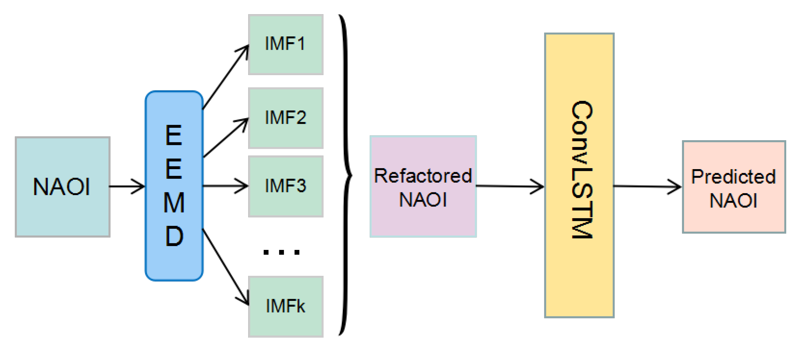
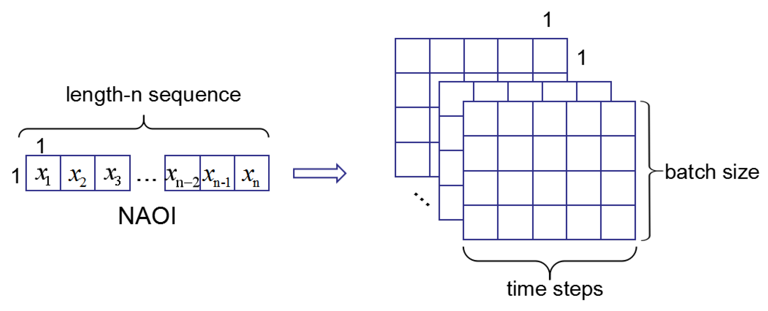
Let us define an NAOI (NAO index) composed of a time series: , where represents the NAO index value at the time point. The objective of NAO index prediction is to predict the value at the next time. We used the EEMD method to decompose data. Firstly, after reconstructing the data, the ConvLSTM was used to extract the features. With the trained model, we can obtain the prediction results. Figure 1 shows the overall network framework. What is more, the input of ConvLSTM is a tensor ∈; is the time step of data; and are the rows and columns of data. The NAO historical data are 1-dimensional vectors, and the output of an EEMD part of the framework is also the 1D vectors. In this paper, we set the input tensor as ∈. Figure 2 shows the input shape. We will use other gird data instead of NAOI to perform further experiments in future.
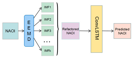
Figure 1.
The architecture of the proposed method. IMF, Intrinsic Mode Function. NAOI, North Atlantic Oscillation index.
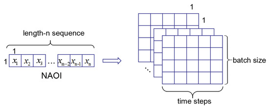
Figure 2.
The input shape of dataset.
2.2. Ensemble Empirical Mode Decomposition Component
The Empirical Mode Decomposition (EMD) method was proposed by Huang et al. [26]. It is a new time-frequency analysis method and an adaptive time-frequency localization analysis method. The EMD decomposes any time series into a sum of a high-frequency part and a low-frequency part. The former is called the IMFs, and the low-frequency part is called the residual. Each IMF is defined by following two requirements: (i) the number of extreme points (maximum or minimum) and zero-crossings of the signal must is equal or differs at most by one; (ii) the average value of the envelope composed of the local maximum value and the local minimum value is zero. Although EMD resolved limitations of the Fourier transform, it cannot decompose signals without enough extreme points; this condition may cause mode mixing and results in inaccurate IMFs. In order to solve this problem, Huang proposed EEMD later [27]. He introduced white noise into the signal. The spectrum of white noise is uniformly distributed, thus making the signal automatically distributed to the appropriate reference scale. Because the zero-mean noises can cancel each other after being calculated by multiple ensemble average, so the calculation result of the ensemble mean can be regarded as the decomposing result directly. What is more, the difference between the ensemble mean and the original signal decreases as the number of ensemble averages increases. The steps of the EEMD algorithm are as follows:
Step 1: Adding a normally-distributed white noise series to the original signal :
Step 2: The signal with white noise as a whole; then, it is decomposed by EMD to obtain each IMF :
Step 3: Repeat Step 1 and Step 2 for a predefined number N of trials; we add a new white noise series for every time;
Step 4: The ensemble mean of each obtained IMFs is used as the final result:
For other data processing methods, such as WT, although this method is widely used in many fields, EEMD was proposed as an alternative method to WT, mainly because the WT decomposes the data needed to select the appropriate mother wavelet and set the feasible decomposition layer. These factors affect the efficiency of this method. While EEMD does not, it is an adaptive method that uses the original data as the “base” to decompose data.
For the proposed model, we used the EEMD method to decompose data. Firstly, we obtained the corresponding residual and a series of IMFs. Then, we calculated the energy value of each IMF . The equation is as follows:
We set the sum of total as , and the threshold represents the ratio of the energy value of IMF to the total energy:
where we selected several IMF , for which , to reconstruct new data. These selected IMFs had a similar structure to the original data, while those IMFs whose energy value was too small were considered as noises, which were not related. In this part, we will get a reconstructed sequence of vectors: .
2.3. Convolutional LSTM Component
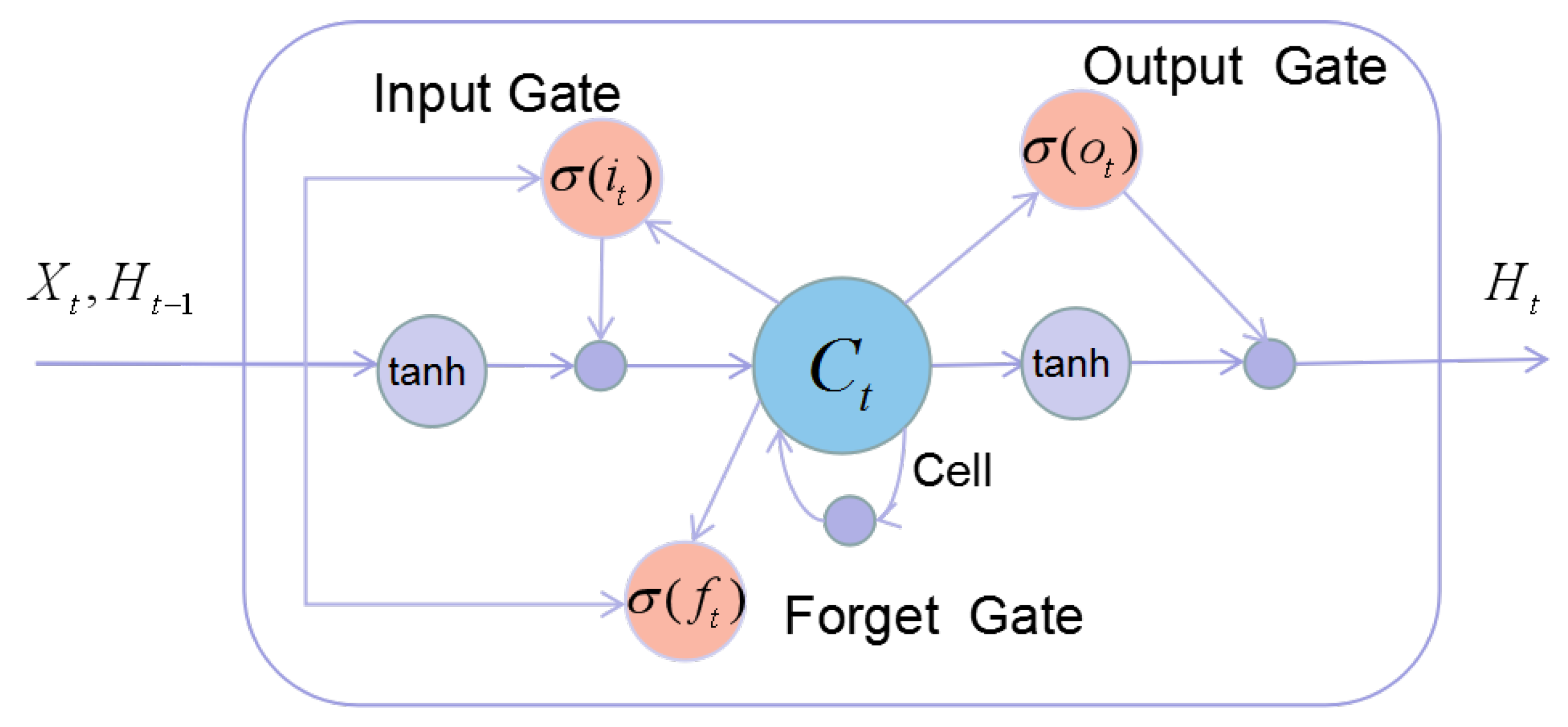
In this model, ConvLSTM was used to capture the temporal dependency in the dataset. It not only can establish the timing relationship like LSTM, but also obtain local spatial features like CNN. The main idea of ConvLSTM is the usage of the convolutional operation instead of the fully-connected one in LSTM. Figure 3 shows the architecture of LSTM. In other words, ConvLSTM can be viewed as a convolution layer embedded with an LSTM. The differences between it and LSTM are that the internal gates of ConvLSTM are the 3D tensor; thus, matrix multiplication is replaced by a convolution operator in the formula of LSTM. The main formula for ConvLSTM is shown as follows:
where ∗ represents the convolution operation and denotes the Hadamard product. is the input gate; is the forget gate controlling the memory; is the output gate; and is the cell state. Function and tanh are two kinds of activations: calculates the element-wise sigmoid activation, and tanh calculates the element-wise hyperbolic tangent activation. stands for the input of current time t, and is the hidden state carried over to the next LSTM and used to generate output. W’s are the weight matrices and b’s the bias terms; they are trainable parameters in neural networks. In the grid, ConvLSTM used the convolution operation to determine the future states of a certain cell with respect to current inputs and the past states of its local neighbors.
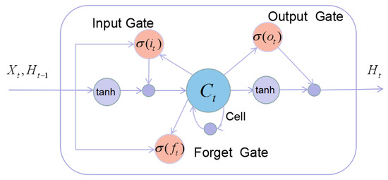
Figure 3.
The structure of LSTM.
2.4. Rolling Forecast
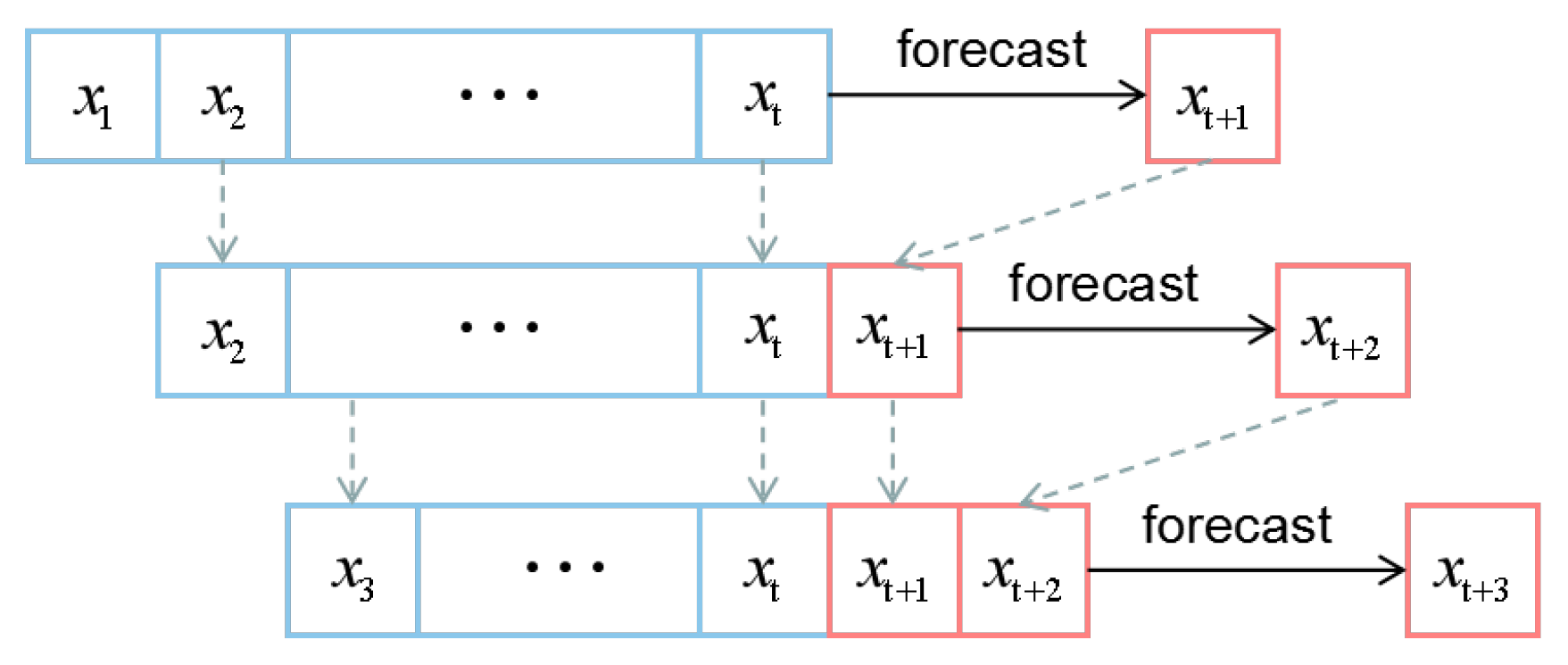
For multi-step time series forecast, most predictive model take some number of observations as input and predict a single output value. As such, they cannot make the forecast directly. In this paper, we propose the Rolling Forecast (RF) based on EEMD-ConvLSTM. We set the input series as a sliding window the the length of t. As we made forecasts with the model, the forecast value was added to the end of this sliding window list, and at the same time, the first value of this list was removed. In this way, the sliding window kept the length unchanged, and we could make multi-step time series forecasts by repeating this process. The diagram of RF is shown in Figure 4
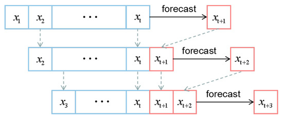
Figure 4.
The process of the rolling forecast.
3. Experiments and Evaluations
3.1. Dataset and Preprocessing
The dataset was the NAO index data, which were supplied by the National Oceanic and Atmospheric Administration (NOAA) [28]. We selected the daily data from 1 January 1950 to 31 August 2018 to analyze the proposed model. The dataset, which contained 25,079 samples, was divided into two sets (training and testing), the former containing 23,741 samples and the latter containing 1338 samples. The descriptive statistics of the NAO index data are shown in Table 1.

Table 1.
The descriptive statistics of the NAO index data.
At first, we needed to normalize the data and use the standardized data for data training before prediction. Min-max normalization, also called dispersion normalization, was used. It is a linear transformation of the original data, so that the result falls into the [0,1] interval:
where is the maximum value of the data and is the minimum value. After the prediction, anti-normalization needs to be used to obtain the true value. The conversion function is as follows:
3.2. Experiments’ Evaluation
There were four evaluation metrics in this experiment to value error and trend performance, which were the Root Mean Squared Error (), Mean Absolute Error (), Explained Variance (), and the Theil Inequality Coefficient (). The corresponding formulas are given as follows:
where and are the real value and the predicted value at time t, respectively. N means the number of data, and VAR() means the Variance of data. The smaller value and value indicate less deviation between the predicted result and the actual value. For , the best score was 1.0; lower values are worse. In addition, the closer the value of is to 0, the higher the precision. On the contrary, the closer the value of is to 1, the lower of precision.
In addition, we ran the LSTM, ConvLSTM, and EEMD-ConvLSTM several times and calculated the variance of their prediction results of RMSE to evaluate them. For the traditional statistical models, General Regression Neural Network (GRNN) and eXtreme gradient boosting (Xgboost), training their data was a process of calculation using mathematical formulas. Therefore, if the dataset is stationary, we will get the same model as the last time trained and get the same prediction results. Thus, we evaluated these models with , , , and , except for variance.
3.3. Parameters Details
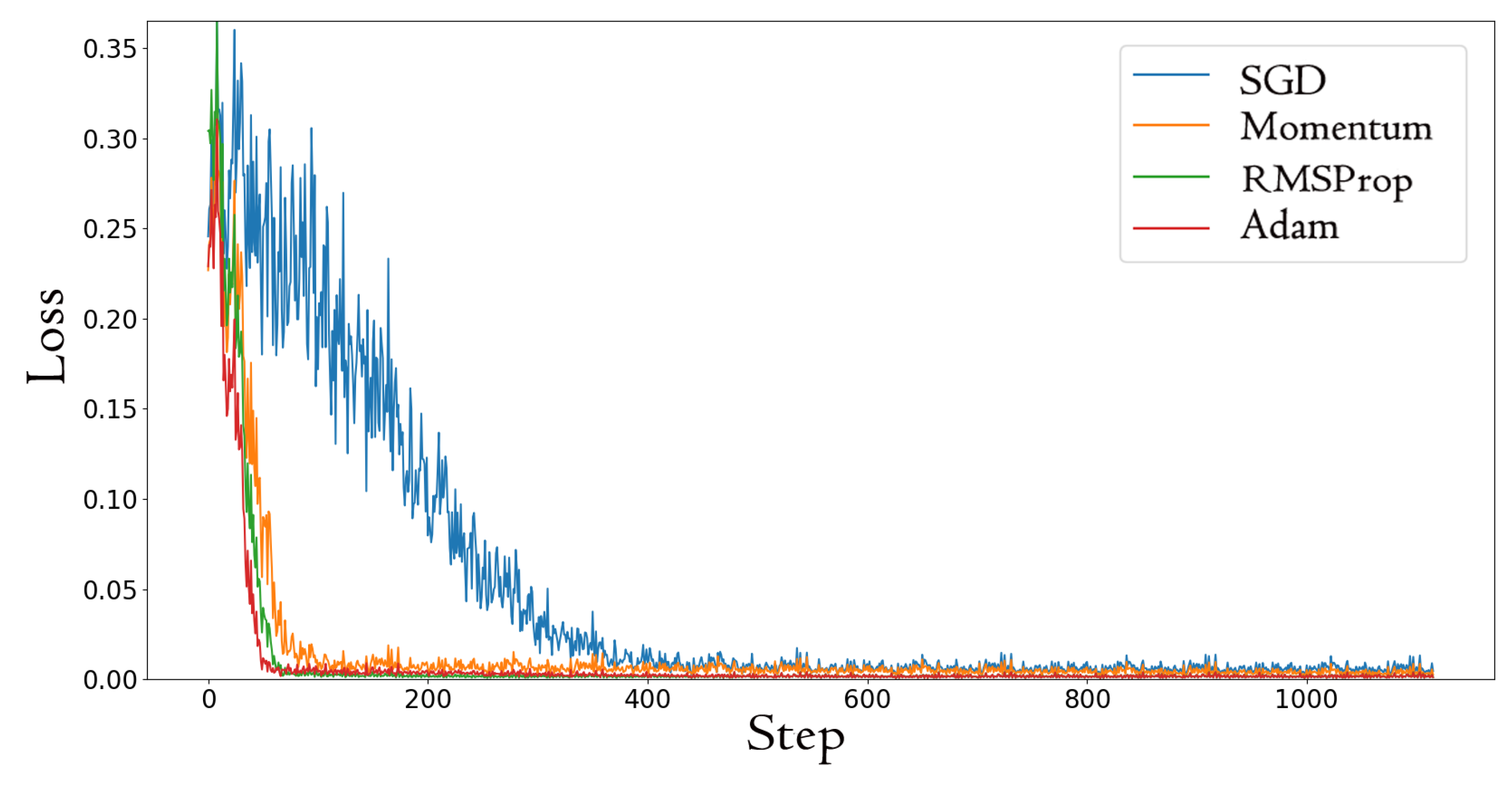
Our implementation was based on the Pytorch framework [29]. As reducing the learning rate or increasing the batch are effective ways to prevent the gradient explosion, these methods can help train the model more robustly. In our model, we trained our networks from scratch using mini-batches of 512 clips, with the initial learning rate as . Because the essence of the machine learning training process is to minimize the loss, after defining the loss function, we needed to set the optimizer to solve the parameters’ optimization problem. In the deep learning library, there is a large number of optimization algorithms, such as Stochastic Gradient Descent (SGD), momentum, root mean square prop (RMSProp), Adaptive Moment Estimation (Adam), etc. In order to select the best optimizer that can not only achieve the best model with the fastest number of training samples, but also prevent over-fitting, we conducted a comparative experiment. Figure 5 shows the results.

Figure 5.
The MSE loss of different optimizers.
From Figure 5, we found that SGD was fluctuating greatly, and the Adam method was the best. Adam is a method for efficient stochastic optimization; the method computes individual adaptive learning rates for different parameters from estimates of the first and second moments of the gradients [30]. As a result, the Adam optimizer is used in the proposed model, and it can converge to a good result much faster.
On this basis, in order to obtain the restructured data, we conducted multiple sets of experiments to choose the best with the above model. The results are shown as Table 2. We found that the was the best choose. In detail, if the threshold is more than 0.03, the IMF, which reflects the original data structure feature, will be discarded. If too small, the useless IMF will be introduced, which is not conducive to signal reconstruction.

Table 2.
The prediction results with different values of . EV, Explained Variance; TIC, Theil Inequality Coefficient.
3.4. Experiments’ Design
At first, we evaluated our EEMD-ConvLSTM model and compared it with the other six prediction models, including the Second Exponential Smoothing (Second-ES) model, the Holt–Winters model, the General Regression Neural Network (GRNN), the eXtreme gradient boosting (Xgboost) model [31], the LSTM model, and the ConvLSTM model. The ES and Holt–Winters model are traditional statistical models, and GRNN, LSTM, and ConvLSTM model are deep neural network models. Furthermore, the Xgboost model is a machine learning algorithm of decision trees. For these experiments, the dataset was the NAO daily data from 1 January 1950 to 14 August 2018, which contains 25,063 samples. To better compare the prediction performance of the proposed model and make sure that the performance difference was only due to the architecture difference instead of fine-turned parameters, we trained these models on the same platform and dataset, and all the involved models were optimized.
Secondly, in order to explore the performance of the NAO index forecast between deep neural networks and numerical models, we compared EEMD-ConvLSTM-RF with two numerical simulations of the NOAA Climate Prediction Center (NOAACPC). NOAACPC uses the averaging of 11 Medium Range Forecast (MRF) model ensemble members (ENSM) and the NCEP’s Global Forecast System (GFS) and provides 7-day, 10-day, and 14-day forecasts. The dataset of the forecast experiments was from 15 to 31 August 2018, which contained 16 samples.
4. Experiments Result and Analysis
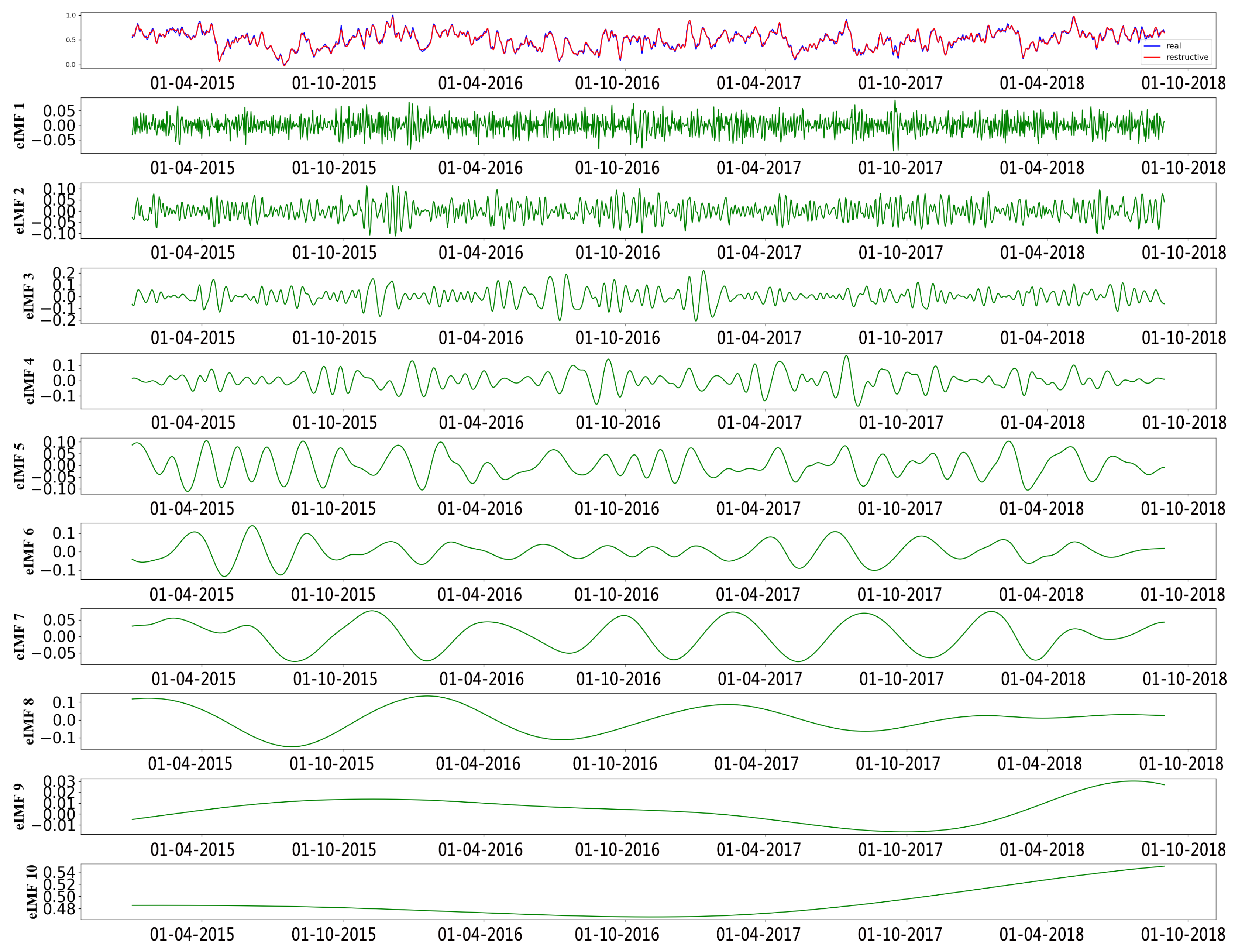
Figure 6 shows the IMFs and the residual of the NAO index data decomposed by EEMD. We can find that the fluctuation frequency gradually reduced from IMF1 to IMF10. According to Equations (4) and (5), we calculated the energy value of IMFs and selected some of them, which matched the criteria to reconstruct the new data, as the input of the proposed model. The first line of Figure 6 displays the original data (blue lines) and restructured data (red lines).
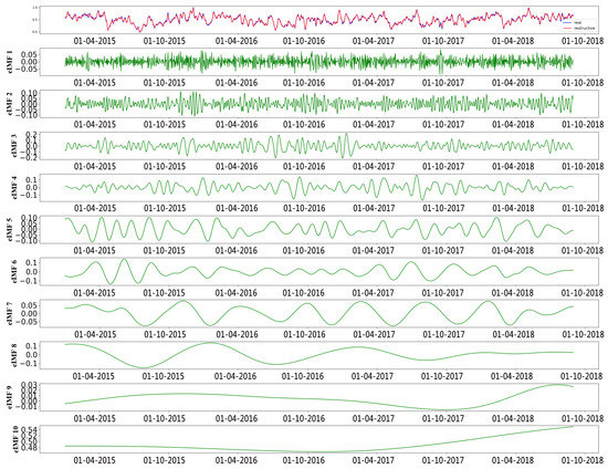
Figure 6.
The decomposing results of the NAO index with EEMD.
The RMSE, MAE, EV, and TIC of different time series prediction models in the experiments are shown in Table 3. In addition, the variance as VAR is also shown in Table 3.

Table 3.
The four evaluation metrics of different models. Second-ES, Second Exponential Smoothing; GRNN, General Regression Neural Network; Xgboost, eXtreme gradient boosting.
From Table 3, comparing the statistical indicators between different models, the values of RMSE and MAE in the EEMD-ConvLSTM were smaller than those in the other models. It is also noted that EEMD-ConvLSTM outperformed the other models for NAO index prediction. What is more, the EV of the EEMD-ConvLSTM was 0.9124, which was the closest to one. The value of TIC in EEMD-ConvLSTM was the smallest and the nearest to zero. Specifically, the VAR of ConvLSTM was the lowest one, and this model was more stable. Though the VAR of EEMD-ConvLSTM was lager than that of ConvLSTM, it was smaller than LSTM, and the proposed method had great stability.
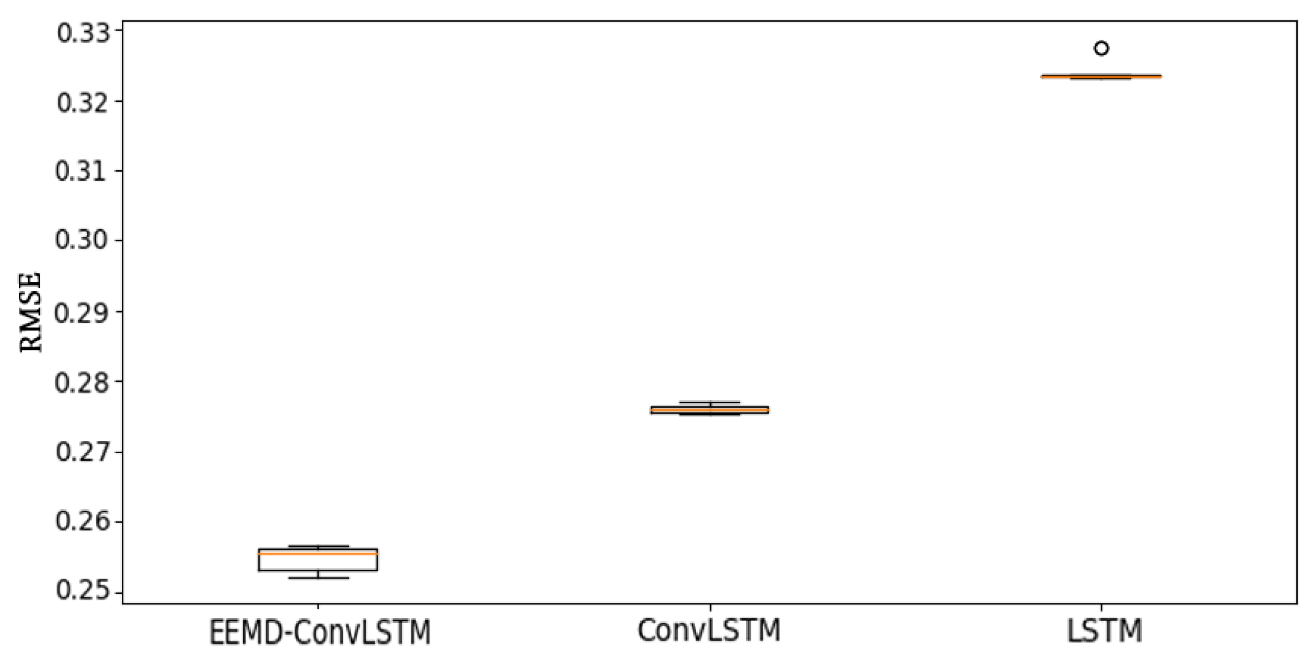
What is more, Figure 7 shows the distribution of the prediction results of RMSE with EEMD-ConvLSTM, ConvLSTM, and LSTM. The red line in the middle of the box represents the median value of the RMSE. The top lines and end lines of the box represent the maximum and minimum of the data (but for one exception). The extreme values or outliers we identified by an asterisk (o). From Figure 7, we can find that the RMSE of EEMD-ConvLSTM was the lowest one, and it had a reliable stability for predicting the NAO index.
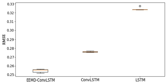
Figure 7.
The box-plot of prediction results of RMSE with different models.
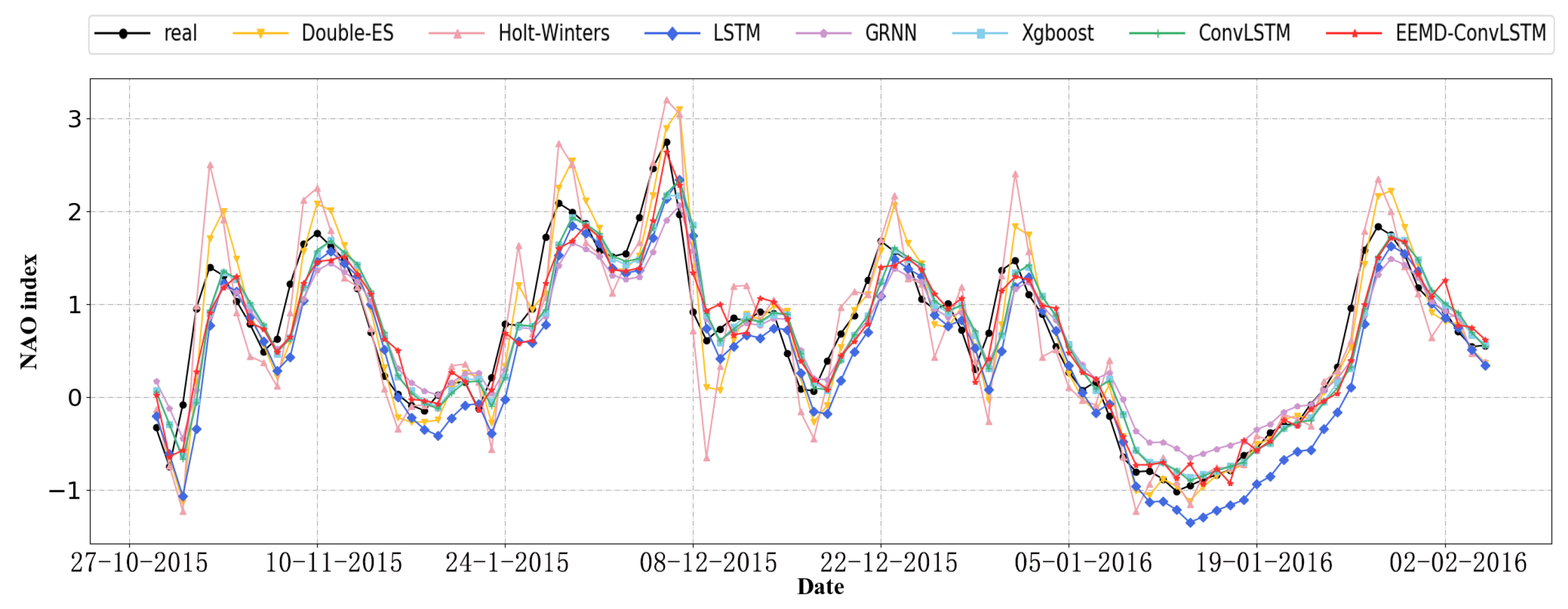
In order to show the differences between different models more intuitively, we plotted a line chart to present the prediction results, and the real values are presented. Specially, their 100-day predictions, which were from October 2015 to February 2016, are shown in Figure 8. From this figure, it is illustrated that the predicted value of EEMD-ConvLSTM and the real data were closer than the other models. Particularly, there was a peak because the NAO index abruptly changes, and it becomes near in early December 2015. Only the prediction of EEMD-ConvLSTM fit well at the peak. For other models, especially the traditional time series model, their prediction results were obviously noisy, while the prediction results of the proposed model were more stable and had a trend similar to the real data.
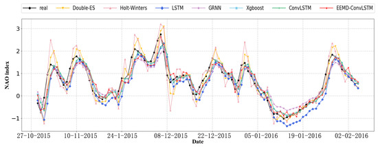
Figure 8.
The 100-day prediction results of different models.
Furthermore, comparing the prediction results between the LSTM, ConvLSTM, and EEMD-ConvLSTM models, the RMSE by LSTM and ConvLSTM were 0.3755 and 0.2755; this means that the ConvLSTM had more reliable performance than LSTM. For the EEMD-ConvLSTM model, the RMSE reduced to 0.2532, which was the lowest one. It clearly justifies the efficiency of the proposed model design, and all components contributed to the excellent and robust performance of EEMD-ConvLSTM. In summary, from the evaluation metrics and prediction line charts, the predictions of EEMD-ConvLSTM was the most reliable.
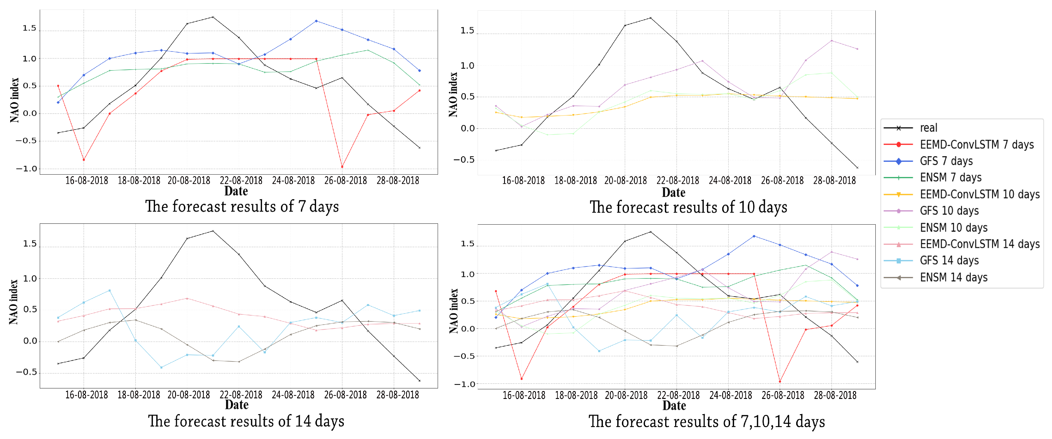
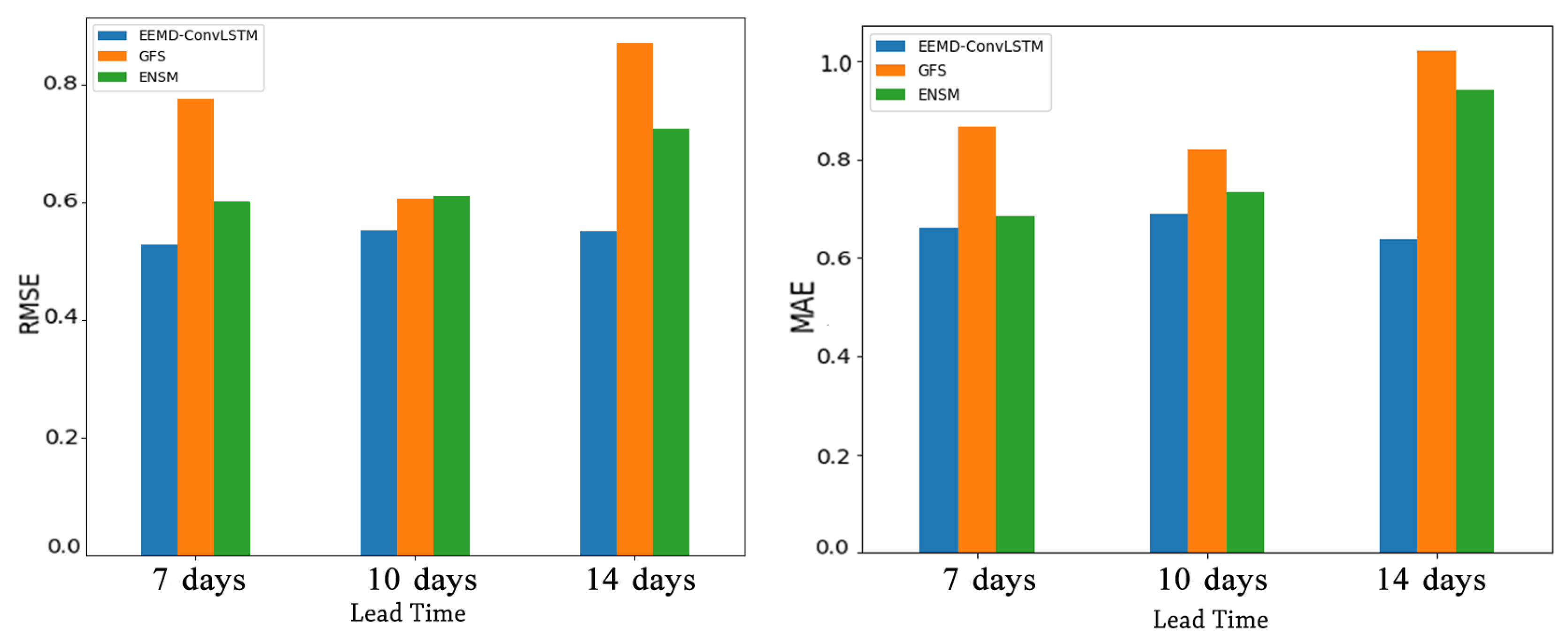
Finally, we compared the effects of different lead times of forecast on the proposed method with rolling forecast and two numerical simulations as shown in Figure 9 and Figure 10. From Figure 9, we note that only the seven-day forecast of our model and the 10-day forecast of GFS extracted the increased trend near 22 August 2018 successfully. According to Figure 10, the RMSE of the latter one was 0.8196, which had a larger deviation, while the former one’s RMSE was 0.6612. Thus, the best forecast performance was obtained by using the proposed model with the RF of the seven-day forecast.
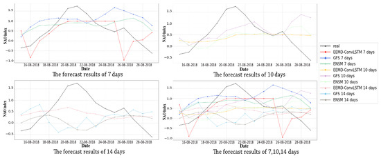
Figure 9.
The forecast results of different models. GFS, Global Forecast System (GFS). ENSM, The averaging of 11 Medium Range Forecast (MRF) model ensemble members (ENSM).
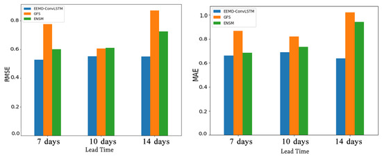
Figure 10.
The RMSE and MAE of forecast results with different models.
Since the forecast error increased with the longer lead time [32], the 10-day and 14-day forecast of these models were not particularly reliable. In addition, from Figure 10, for the 14-day forecast of GFS and ENSM, their performance was roughly the same. They had larger RMSE and MAE. These imply that they cannot forecast the NAO index reliably; whereas the performance of the 10-day forecast of GFS and ENSM was average. For the 10-day and 14-day forecasts of the proposed model, their forecast results were relatively moderate, and they had similar performance.
Although the forecast results of the proposed model still had a certain gap with the real data, they were better than GFS and ENSM in terms of evaluation metrics. It is difficult to forecast the NAO index with a long lead time, and the NOAA Climate Prediction Center provides the GFS and ENSM of these two numerical simulations to forecast the NAO index; although they are already mature forecast models, they also cannot obtain reliable forecast results. However, our proposed method had superiority over these numerical simulations. In the future, we will use other grid data to calculate the NAO index instead of using the NAO index directly, and we also will use multivariable data to help the accuracy improvement for NAO forecast.
5. Conclusions
In this paper, an effective neural network model, EEMD-ConvLSTM, which is based on ConvLSTM with EEMD, was established aiming at predicting the fluctuations of the NAO index. NAO index data were preprocessed by EEMD. They were decomposed into several IMFs, and these IMFs were filtered by the energy threshold, then the remaining IMFs were used to reconstruct new NAO index data as the input of ConvLSTM. To validate the experiment results, four evaluation metrics (RMSE, MAE, EV, and TIC) were used. Besides the real data, the predictions of our model were also compared with another six methods, which included traditional models (Second ES, Holt–Winters), a machine learning algorithm (Xgboost), and other deep neural networks (GRNN, LSTM, ConvLSTM). The experiment results demonstrated that EEMD-ConvLSTM model had the highest reliability; the value of the RMSE was the lowest at 0.2532, and the results for ConvLSTM were superior to those of LSTM. This also indicates that EEMD and convolution layers in the EEMD-ConvLSTM model are productive. We also forecast the NAO index with a lead time of 7 days, 10 days, and 14 days in the EEMD-ConvLSTM model and rolling forecast. We compared the results with GFS and ENSM, which were the ensemble forecasts of multiple numerical models. The experiment results revealed that the EEMD-ConvLSTM model was much better than the compared models. There also exists a general problem in meteorology that the forecast error increases with a longer lead time. In the future, we will focus on further improving the reliability of NAO index prediction. More meteorological elements that are related to NAO events will be considered in the EEMD-ConvLSTM model. In addition, we will design more suitable network structures.
Author Contributions
X.L. wrote the original manuscript and designed the network model; X.L. and J.L. performed the experiments and validation; B.M. and S.Y. supported the project and reviewed and edited the manuscript. We also thank the help of G.D. as an expert in the area of atmosphere.
Funding
The work was supported by the National Natural Science Fund of China (No. 41405097).
Conflicts of Interest
The authors declare no conflict of interest.
References
- Walker, G. World weather. Mon. Weather Rev. 1928, 56, 79–87. [Google Scholar] [CrossRef]
- Woollings, T.J.; Hoskins, B.J.; Blackburn, M.; Berrisford, P. A New Rossby Wave-breaking Interpretation of the North Atlantic Oscillation. J. Atmos. Sci. 2008, 65, 609–626. [Google Scholar] [CrossRef]
- Wu, Z.; Wang, B.; Li, J.; Jin, F. An Empirical Seasonal Prediction Model of the East Asian Summer Monsoon Using ENSO and NAO. J. Geophys. Res. Atmos. 2010. [Google Scholar] [CrossRef]
- Sillmann, J.; Crocimaspoli, M. Present and future atmospheric blocking and its impact on European mean and extreme climate. Geophys. Res. Lett. 2009, 36, 92–103. [Google Scholar] [CrossRef]
- Wang, C.; Liu, H.; Lee, S. The record-breaking cold temperatures during the winter of 2009/2010 in the Northern Hemisphere. Atmos. Sci. Lett. 2010, 11, 161–168. [Google Scholar]
- Hurrell, J.W. Decadal Trends in the North Atlantic Oscillation: Regional Temperatures and Precipitation. Science 1995, 269, 676–679. [Google Scholar] [CrossRef] [PubMed]
- Scaife, A.A.; Arribas, A.; Blockley, E.; Brookshaw, A.; Clark, R.T.; Dunstone, N.; Eade, R.; Fereday, D.; Folland, C.K.; Gordon, M. Skilful Long Range Prediction of European and North American Winters. Geophys. Res. Lett. 2014, 41, 2514–2519. [Google Scholar] [CrossRef]
- Fereday, D.R.; Maidens, A.; Arribas, A.; Scaife, A.A.; Knight, J.R. Seasonal forecasts of northern hemisphere winter 2009/10. Environ. Res. Lett. 2012, 7, 34031–34037. [Google Scholar] [CrossRef]
- Lin, H.; Brunet, G. Impact of the North Atlantic Oscillation on the forecast skill of the Madden-Julian Oscillation. Geophys. Res. Lett. 2011, 37, 96–104. [Google Scholar] [CrossRef]
- Doblas-Reyes, F.; Pavan, V.; Stephenson, D. The skill of multi-model seasonal forecasts of the wintertime North Atlantic Oscillation. Clim. Dyn. 2003, 21, 501–514. [Google Scholar] [CrossRef]
- Hansen, F.; Greatbatch, R.J.; Gollan, G.; Jung, T.; Weisheimer, A. Remote control of North Atlantic Oscillation predictability via the stratosphere. Q. J. R. Meteorol. Soc. 2017, 143, 706–719. [Google Scholar] [CrossRef]
- Baker, L.H.; Shaffrey, L.C.; Sutton, R.T.; Weisheimer, A.; Scaife, A.A. An Intercomparison of Skill and Overconfidence/Underconfidence of the Wintertime North Atlantic Oscillation in Multimodel Seasonal Forecasts. Geophys. Res. Lett. 2018, 45, 7808–7817. [Google Scholar] [CrossRef]
- Li, C.; Yun, B.; Bo, Z. Deep Feature Learning Architectures for Daily Reservoir Inflow Forecasting. Water Resour. Manag. 2016, 30, 1–17. [Google Scholar] [CrossRef]
- Zhang, Q.; Wang, H.; Dong, J.; Zhong, G.; Sun, X. Prediction of Sea Surface Temperature using Long Short-Term Memory. IEEE Geosci. Remote Sens. Lett. 2017, 14, 1745–1749. [Google Scholar] [CrossRef]
- Mcdermott, P.L.; Wikle, C.K. Bayesian Recurrent Neural Network Models for Forecasting and Quantifying Uncertainty in Spatial-Temporal Data. Entropy 2019, 21, 184. [Google Scholar] [CrossRef]
- Mcdermott, P.L.; Wikle, C.K. An Ensemble Quadratic Echo State Network for Nonlinear Spatio-Temporal Forecasting. Stat 2017, 6, 315–330. [Google Scholar] [CrossRef]
- Kim, S.; Hong, S.; Joh, M.; Song, S.K. DeepRain: ConvLSTM Network for Precipitation Prediction using Multichannel Radar Data. arXiv 2017, arXiv:1711.02316. [Google Scholar]
- Shi, X.; Chen, Z.; Wang, H.; Yeung, D.Y.; Wong, W.; Woo, W. Convolutional LSTM Network: A Machine Learning Approach for Precipitation Nowcasting. In Proceedings of the International Conference on Neural Information Processing Systems, Montreal, QC, Canada, 7–12 December 2015; pp. 802–810. [Google Scholar]
- Dibike, Y.B.; Coulibaly, P. Temporal neural networks for downscaling climate variability and extremes. Neural Netw. 2006, 19, 135–144. [Google Scholar] [CrossRef]
- Dariouchy, A.; Aassif, E.; Lekouch, K.; Bouirden, L.; Maze, G. Prediction of the intern parameters tomato greenhouse in a semi-arid area using a time-series model of artificial neural networks. Measurement 2009, 42, 456–463. [Google Scholar] [CrossRef]
- Chang, J.; Wang, G.; Mao, T. Simulation and prediction of suprapermafrost groundwater level variation in response to climate change using a neural network model. J. Hydrol. 2015, 529, 1211–1220. [Google Scholar] [CrossRef]
- Liu, H.; Mi, X.; Li, Y. Smart deep learning based wind speed prediction model using wavelet packet decomposition, convolutional neural network and convolutional long short term memory network. Energy Convers. Manag. 2018, 166, 120–131. [Google Scholar] [CrossRef]
- Liu, H.; Mi, X.; Li, Y. Smart multi-step deep learning model for wind speed forecasting based on variational mode decomposition, singular spectrum analysis, LSTM network and ELM. Energy Convers. Manag. 2018, 159, 54–64. [Google Scholar] [CrossRef]
- Wang, D.; Liu, Y.; Luo, H.; Yue, C.; Cheng, S. Day-Ahead PM2.5 Concentration Forecasting Using WT-VMD Based Decomposition Method and Back Propagation Neural Network Improved by Differential Evolution. Int. J. Environ. Res. Public Health 2017, 14, 764. [Google Scholar] [CrossRef]
- Sun, W.; Liu, M. Wind speed forecasting using FEEMD echo state networks with RELM in Hebei, China. Energy Convers. Manag. 2016, 114, 197–208. [Google Scholar] [CrossRef]
- Huang, N.E.; Shen, Z.; Long, S.R.; Wu, M.C.; Shih, H.H.; Zheng, Q.; Yen, N.-C.; Tung, C.C.; Liu, H.H. The Empirical Mode Decomposition and the Hilbert Spectrum for Nonlinear and Non-stationary Time Series Analysis. Proc. Math. Phys. Eng. Sci. 1998, 454, 903–995. [Google Scholar] [CrossRef]
- Wu, Z.; Huang, N.E. Ensemble Empirical Mode Decomposition: A Noise-Assisted Data Analysis Method. Adv. Adapt. Data Anal. 2009, 1, 1–41. [Google Scholar] [CrossRef]
- PSD. NOAA Earth System Research Laboratory’s Physical Sciences Division (PSD). Available online: https://www.esrl.noaa.gov/psd/ (accessed on 11 March 2019).
- Facebook. An Open Source Deep Learning Platform that Provides a Seamless Path from Research Prototyping to Production Deployment. 2017. Available online: https://lornatang.github.io/PyTorch/ (accessed on 11 March 2019).
- Kingma, D.; Ba, J. Adam: A Method for Stochastic Optimization. Mach. Learn. arXiv 2014, arXiv:1412.6980. [Google Scholar]
- Chen, T.; Guestrin, C. XGBoost: A Scalable Tree Boosting System. In Proceedings of the ACM SIGKDD International Conference on Knowledge Discovery and Data Mining, San Francisco, CA, USA, 13–17 August 2016; pp. 785–794. [Google Scholar]
- Bao, Y.; Xiong, T.; Hu, Z. Multi-Step-Ahead Time Series Prediction using Multiple-Output Support Vector Regression. Neurocomputing 2014, 129, 482–493. [Google Scholar] [CrossRef]
© 2019 by the authors. Licensee MDPI, Basel, Switzerland. This article is an open access article distributed under the terms and conditions of the Creative Commons Attribution (CC BY) license (http://creativecommons.org/licenses/by/4.0/).

