Abstract
Hydrologic margins of wetlands are narrow, transient zones between inundated and dry areas. As water levels fluctuate, the dynamic hydrology at margins may impact wetland greenhouse gas (GHG) fluxes that are sensitive to soil saturation. The Prairie Pothole Region of North America consists of millions of seasonally-ponded wetlands that are ideal for studying hydrologic transition states. Using a long-term GHG database with biweekly flux measurements from 88 seasonal wetlands, we categorized each sample event into wet to wet (W→W), dry to wet (D→W), dry to dry (D→D), or wet to dry (W→D) hydrologic states based on the presence or absence of ponded water from the previous and current event. Fluxes of methane were 5-times lower in the D→W compared to W→W states, indicating a lag ‘ramp-up’ period following ponding. Nitrous oxide fluxes were highest in the W→D state and accounted for 20% of total emissions despite accounting for only 5.2% of wetland surface area during the growing season. Fluxes of carbon dioxide were unaffected by transitions, indicating a rapid acclimation to current conditions by respiring organisms. Results of this study highlight how seasonal drying and re-wetting impact GHGs and demonstrate the importance of hydrologic transitions on total wetland GHG balance.
1. Introduction
Concerns over climate change have stimulated considerable research focused on providing a better understanding of the key sources and sinks of biologically produced and consumed greenhouse gases (GHGs) such as carbon dioxide (CO2), methane (CH4), and nitrous oxide (N2O) [1,2,3]. Globally, wetland ecosystems have been recognized as prospective carbon storage sites where carbon uptake exceeds losses. Wetlands, however, have the potential to emit and consume significant amounts of potent GHGs such as CH4 and N2O [3,4,5,6]. Therefore, the ability to accurately estimate the overall GHG balance of wetland ecosystems is necessary to determine their role as radiative sources or sinks.
Wetland systems often are distinguished by highly dynamic GHG fluxes that display substantial temporal and spatial variability. This variability has been associated with a myriad of factors including abiotic conditions (e.g., soil moisture and temperature), biotic communities (e.g., microbial, vegetation), emission pathway (diffusive flux, ebullition, and plant-mediated flux), wetland type (e.g., peatland, mineral-soil, tidal), and weather [4,6,7,8,9,10,11]. Wetland hydrology, specifically inundation or ponding, is a primary factor that directly and indirectly influences the GHG and carbon balance of wetland systems [4,12]. Throughout the growing season, many wetlands are typified by fluctuations between ponded and dry conditions, which are often separated by a moving, hydrologic transition area, or moist-margin [13]. This intermediate area may function as a hot spot for GHG production and flux that differs from the adjacent ponded and dry areas [14]; thus, while the areal coverage of this transition area may be relatively small, it may have a disproportionate contribution to overall wetland GHG fluxes. Despite this, few studies have examined abiotic conditions or GHG fluxes of hydrologic transition areas.
The Prairie Pothole Region (PPR) of North America has been identified as an area of interest owing to its potential role in the continental GHG budget [6,15,16]. The PPR, which encompasses approximately 800,000 km2 of the United States and Canada, is characterized by millions of small, mineral-soil wetlands embedded within a landscape composed of cropland and grassland. Wetlands of the PPR can be highly productive, and consequently are capable of sequestering atmospheric carbon in soils and vegetation [15,16]. These wetlands can also be sources or sinks of GHGs, most notably CH4 and N2O. Studies have demonstrated considerable temporal variation in GHG flux of PPR wetlands, and have recognized relations between flux and factors such as soil moisture, temperature, water depth, and land use. Although we are unaware of any studies that specifically examine GHG flux from hydrologic transition areas of PPR wetlands, Bansal et al. [11] demonstrated differences in CH4 flux among saturation states (ponded, semi-saturated, and dry) of a seasonal PPR wetland, and Pennock et al. [8] associated N2O flux events with areas of PPR wetlands that were distinguished by rapid soil drainage.
Most wetlands in the PPR are classified as seasonal (i.e., ponds completely dry during most years) [17,18], with concentric zones consisting of distinct vegetation communities that vary based on hydrology and soil properties. PPR wetlands are fed through atmospheric inputs from snowmelt runoff and precipitation, and evapotranspiration exceeds precipitation in the region [13,19,20]. Therefore, a large proportion of wetlands draw down (i.e., water levels recede) or completely dry seasonally (Figure 1), depending on the magnitude of inputs (precipitation, runoff) and losses (evapotranspiration, recharge) [13]. As water levels fluctuate, the vegetation zones transition between wet, moist-soil, and dry conditions. Thus, PPR wetlands are ideal microcosms for studying the effects of hydrological transitions.
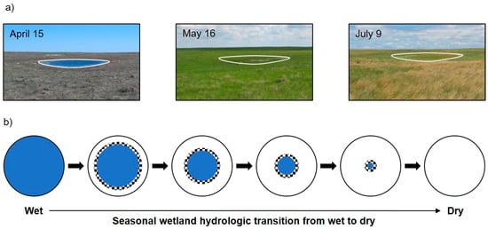
Figure 1.
(a) Time series photographs (circa 2007) of a seasonally-ponded Prairie Pothole Region wetland located in native prairie grasslands in South Dakota, USA. The time series depicts water-level drawdown throughout the ice-free season, which is characteristic of many seasonal wetlands. In this example, water depths gradually declined from approximately 33 cm during April until the site dried during early July; the wetland remained dry throughout the remainder of the season. (b) Depiction of ponded (blue) and dry (white) portions of a depressional wetland basin along a seasonal hydrologic gradient from ponded to dry; the checkered area represents the transition area between the ponded and dry areas (i.e., wet to dry). PPR wetlands often begin the ice-free season with high water levels from snowmelt runoff and spring precipitation. Water levels typically recede throughout the year because evapotranspiration exceeds precipitation.
Previous research has demonstrated variation in GHG fluxes among vegetation zones and landscape elements of PPR wetlands [6,16,21,22,23]. Studies have also identified areas of partially-saturated soils as potential hot spots for GHG flux [8,11,14]. The goal of this study was to assess GHG fluxes from hydrologic and transition states (i.e., wet to wet, dry to wet, dry to dry, or wet to dry) of PPR wetlands. To accomplish this goal, we analyzed a published, long-term database consisting of GHG fluxes (CH4, N2O, CO2) and associated hydrologic data from seasonal PPR wetlands [24].
2. Data and Methods
2.1. GHG Data
We obtained data for this study from a published, comprehensive database of wetland GHG fluxes [24]. The studies that constitute this database have resulted in numerous peer-reviewed publications detailing GHG fluxes of PPR wetlands [6,10,11,25,26,27,28]. This database includes CH4, N2O, and CO2 fluxes from nearly 200 seasonal and semipermanent (classification of [17]) PPR wetlands that were embedded in grasslands and croplands; data were collected between 2003 and 2016. Flux data were collected using the using the static-chamber approach and abiotic covariates, such as water depth, were provided at the individual sample location (i.e., gas-collection chamber; hereafter, chamber). In addition, we obtained topographic data describing the representative surface areas for each of the chambers (e.g., concentric chamber zones), which were based on mid-point elevations between adjacent chambers [26]. The topographic data were based on detailed surveys performed at each wetland catchment using a GPS survey system. Methodologies among the various studies that comprise these data remained consistent over time, and are detailed by Gleason et al. [25], Finocchiaro et al. [26], Tangen et al. [6], and Tangen and Bansal [24]. Below, we provide a general overview of the gas-collection methods.
Within each wetland catchment, samples were collected and abiotic data were measured along a transect spanning the wetland–upland gradient. Five sample locations were equally distributed between the approximate wetland center and edge, and another three were established at the toe-, mid-, and shoulder-slope positions in the adjacent uplands (Figure 2). When water depths were less than approximately 5 cm, chamber bases were permanently installed at the beginning of each field season. Mid-day (9:00–16:00 h) flux measurements were made biweekly (every 2 weeks) throughout the ice-free season. For flux measurements, opaque polyvinyl chloride chambers (20-cm diameter, 20-cm height) were attached to bases, or when water depths exceeded 5 cm the chambers were attached to floats. When using floats, chambers were deployed and secured to previously-installed poles using a pully system to minimize disturbance to the underlying sediments. Chambers were deployed for approximately 30 min after which headspace gas samples were collected using a syringe through a rubber septum and transferred to pre-evacuated 10-mL glass bottles. Gas samples were analyzed within 3 weeks of collection using a gas chromatograph equipped with electron capture and flame ionization detectors (SRI 8610C, SRI Instruments, Torrance, CA).
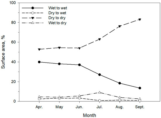
Figure 2.
Average monthly (arithmetic mean) percent of total surface area for the wet to wet, dry to wet, dry to dry, and wet to dry states of seasonal Prairie Pothole Region wetlands.
2.2. Database Modification
The comprehensive database [24] was modified as follows. We included only seasonal wetlands owing to their regional abundance and hydrologic characteristics that result in distinctive water-level declines during most years. We retained only data for the five wetland-zone samples (chambers 1–5) collected from April through September, and for wetlands where data were available for all five sample locations (i.e., no missing values). For this subset of data, we determined the sample interval (days between repeated sample events) for corresponding samples, and removed samples separated by less than 12 or greater than 16 days (10th and 90th quantiles). The remaining data approximate the standard biweekly sampling scheme used for most of the associated studies [24]. We also removed data collected from drained wetlands because of the disrupted hydrology, which could confound analyses presented in this paper. The resulting database consisted of 9,840 samples (five samples/wetland/date) from 88 seasonal wetlands distributed across North and South Dakota, Minnesota, and Iowa. Of these wetlands, 17 were sampled for 1 year, 45 for 2 years, 20 for 4 years, and 6 for 8 years. Wetlands were distributed among various land uses including native prairie (n = 24), restored grasslands (n = 41), and cropland (n = 23). For the wetlands included here, average soil organic carbon, nitrogen, and bulk density in the upper 15 cm of the soil profile was 5.04% (se ± 0.23), 0.45% (se ± 0.02), and 0.95 g cm−3 (se ± 0.02), respectively [24]. Combining data from a range of studies facilitates the identification of robust trends across a range of climatic conditions, geographic locations, and soils that are representative of the PPR. The previously-mentioned topographic data were available for 84 of the 88 wetlands. On average, 74% of the 88 wetlands dried each year, although 0–100% dried during any given year. Moreover, 95% of the wetlands dried at least once during the various studies conducted from 2003–2016 (Table 1). A wetland was considered dry when all sample locations were dry (water depth = 0), although the soils may have been saturated or partially saturated.

Table 1.
Number of seasonal Prairie Pothole Region wetlands that dried (Dried) and remained at least partially inundated (Wet), by year, and that dried at least once during the study period (2003–2016). Percent dried is the percentage of wetlands that dried by year, and during the study period.
2.3. Analyses
To facilitate analyses based on changing hydrologic conditions, we created a hydrologic state variable to categorize each sample based on water depths of the previous and current sample dates (~2-week interval) within each season. Sample locations that remained ponded or unponded between sampling dates were categorized as wet to wet (W→W) or dry to dry (D→D), respectively. Sample locations that transitioned between ponded and unponded conditions were categorized as wet to dry (W→D) or dry to wet (D→W).
To demonstrate seasonal hydrologic variability, we determined the areal extent of the four hydrologic states and calculated the average monthly percentages of total wetland surface area that were in each hydrologic state. Surface areas were determined using the aforementioned topographic survey data collected at each wetland. We also tested for differences in CH4, N2O, and CO2 fluxes among the four hydrologic states using analysis of variance (ANOVA) methods. In the models, the repeated samples (several years and multiple dates within years) were treated as subsamples in time, and wetland and sample location (chamber) were considered random effects. Prior to analyses, CH4, N2O, and CO2 fluxes were natural log transformed after adding a nominal value to make fluxes positive. Least square means (LSM) were back transformed for data presentation and statistical significance was inferred using α = 0.05. Furthermore, we calculated average monthly flux for each hydrologic state, as well as an overall flux for all states combined. Lastly, we estimated an average cumulative seasonal (April–September) flux (CH4, N2O, and CO2) for each hydrologic state that incorporated the surface area of each state. To do this, we calculated average surface area (m2) of each hydrologic state based on daily wetland totals; if a hydrologic state did not occur for a given wetland/date combination a value of zero was assigned for that state. We then scaled the average GHG flux (LSM; mg CH4/CO2 or μg N2O m−2 hr−1) to a daily flux (24 h) and multiplied it by the average daily area of each hydrologic state. The resulting average flux per wetland per day was multiplied by 183 days to approximate the average seasonal flux for each hydrologic state.
3. Results
3.1. Hydrology
The average percentage of wetland surface area in the W→W hydrologic state decreased from April (40%) through September (14%) while the percentage of wetland surface area in the D→D hydrologic state increased from 53% to 83% (Figure 2). The percentage of W→D wetland surface area peaked in July (9%) as wetland water levels receded. The percentage of D→W wetland area was 3% from April through June and 1% from July through September (Figure 2).
3.2. Greenhouse Gas Fluxes
Fluxes of CH4 (F3,214 = 126.44, p < 0.01), N2O (F3,214 = 110.04, p < 0.01), and CO2 (F3,214 = 232.07, p < 0.01) varied significantly among the four hydrologic states (Figure 3a–c). CH4 flux was greatest from the W→W state (14.92 mg CH4 m−2 hr−1, 95% confidence interval [CI] = 11.58–19.11), followed by the W→D (6.86 mg CH4 m−2 hr−1, [CI] = 5.12–9.06), D→W (3.02 mg CH4 m−2 hr−1, [CI] = 1.94–4.45), and D→D (0.31 mg CH4 m−2 hr−1, [CI] = −0.03–0.74) states. On average, CH4 flux from the W→W state was nearly five times greater than the D→W state, and flux from the W→D state was 22 times greater than the D→D state (Figure 3a). N2O flux was greatest from the W→D state (92.37 μg N2O m−2 hr−1, [CI] = 81.54–103.84), followed by the D→D state (29.25 μg N2O m−2 hr−1, CI = 23.29–35.50); the D→W (4.28 μg N2O m−2 hr−1, [CI] = −3.08–12.20) and W→W (−0.62 μg N2O m−2 hr−1, [CI] = −5.90–4.96) states were similar and characterized by very low N2O flux (Figure 3b). N2O flux from the W→D state was over three times greater than the D→D state. CO2 fluxes from the D→D (644.43 mg CO2 m−2 hr−1, [CI] = 607.36–682.95) and W→D (688.93 mg CO2 m−2 hr−1, [CI] = 636.31–744.38) states were greater than those from the W→W (229.02 mg CO2 m−2 hr−1, [CI] = 204.16–255.00), and D→W (215.96 mg CO2 m−2 hr−1, [CI] = 177.49–257.28) states (Figure 3c). When combined, CO2 flux from the D→D and W→D states was three times greater than flux from the W→W and D→W states. There were no differences in CO2 flux between the D→D and W→D or between W→W and D→W states (Figure 3c).
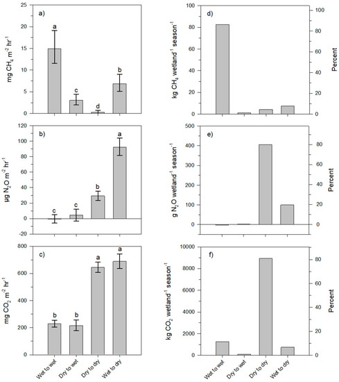
Figure 3.
Average (least square means ± 95% confidence intervals) fluxes of (a) CH4, (b) N2O, and (c) CO2 of seasonal Prairie Pothole Region wetlands by hydrologic state. Average area-adjusted, cumulative fluxes of (d) CH4, (e) N2O, and (f) CO2 of seasonal Prairie Pothole Region wetlands by hydrologic state. For panels a–c, different letters indicate significant differences among the hydrologic states (α = 0.05).
The overall fluxes (Figure 3a–c) represent average fluxes for a hydrologic state while the average area-adjusted cumulative fluxes (Figure 3d–f) incorporate the contributing surface area of each hydrologic state over time (Figure 2). Area-adjusted cumulative CH4 flux (Figure 3d) displayed patterns similar to overall flux rates (Figure 3a), although the relative contributions of the hydrologic states differed. Area-adjusted cumulative N2O and CO2 flux, however, displayed dissimilar patterns where the relative contribution from the W→D state was reduced when the area of the hydrologic states was considered (Figure 3b–c,e–f). Based on the area-adjusted cumulative fluxes, the W→D and D→W hydrologic states collectively accounted for 9.0% of CH4 flux, 20.1% of N2O flux, and 7.5% of CO2 flux, while accounting for a combined 7.0% of wetland surface area. The D→W (1.8% of wetland surface area) and W→D (5.2% of wetland surface area) hydrologic states accounted for 1.2% and 7.8% of CH4 flux, respectively (Figure 3d), while the W→W state (26.5% of wetland surface area) accounted for 86.5% of CH4 flux. For N2O, the D→W and W→D hydrologic states accounted for 0.3% and 19.7% of N2O flux (positive flux only), respectively, while the D→D state (66.5% of wetland surface area) accounted for 79.9% of total N2O emissions (Figure 3e). For CO2, the D→W and W→D hydrologic states accounted for 0.7% and 6.8% of CO2 flux, respectively, while the D→D and W→W states accounted for 81.0% and 11.5%, respectively (Figure 3f).
Average monthly fluxes of CH4, N2O, and CO2 generally increased from April through July and declined thereafter (Figure 4a–c). Monthly CH4 fluxes, however, increased throughout the year for the W→W, W→D, and D→W states (Figure 4a). Similarly, monthly N2O fluxes from the W→D state remained relatively high throughout the year (Figure 4b). N2O fluxes from the D→D state, although lower than those from the W→D state, were also relatively stable throughout the year. Monthly CO2 fluxes from all hydrologic states displayed seasonal variability similar to the overall monthly average, and the drier states (D→D, W→D) generally displayed greater average fluxes than the wetter states (W→W, D→W) (Figure 4c).
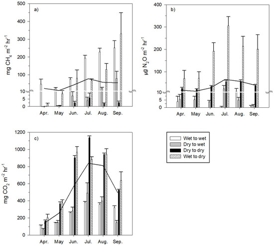
Figure 4.
Average (arithmetic mean ± standard error) monthly (a) CH4, (b) N2O, and (c) CO2 fluxes of seasonal Prairie Pothole Region wetlands by hydrologic state. The solid lines represent the average monthly (arithmetic mean) fluxes based on all sample locations and hydrologic states.
4. Discussion
As the hydrologic condition of a wetland changes over time, so does the spatial distribution of GHG fluxes. Through examination of a long-term database, we demonstrated seasonal variability in PPR wetland hydrology and revealed distinct patterns in GHG fluxes among four hydrologic states (Figure 3a–c). Fluxes of CH4 and N2O were strongly affected by the previous hydrological state and displayed a lag effect, while CO2 was minimally affected by transitions between wet and dry states. These findings demonstrate the importance of considering hydrologic variability or state (e.g., W→W, W→D) when collecting GHG samples, estimating fluxes, or interpreting GHG data of dynamic wetland systems.
4.1. Hydrology and GHG Flux
4.1.1. CH4
It has been well established that CH4 flux from wetlands is influenced by, among other things, soil saturation and temperature, and that seasonal flux often peaks during mid-summer when conditions are optimal for the production of CH4 [6,11,16,25,28,29]. Correspondingly, overall average monthly CH4 fluxes (solid line in Figure 4a) presented as part of this study generally increased from April through July and decreased nearly 30% from July to September (Figure 4a). These qualitative trends, which are based on average wetland fluxes for the entire wetland, suggest that CH4 production and flux decline as the season progresses and abiotic (e.g., temperature, soil moisture) and biotic (e.g., vegetation) conditions change. Yet, when CH4 fluxes are examined in relation to hydrologic state or condition, it is apparent that fluxes can remain high throughout the season in W→W, D→W, or W→D locations (Figure 4a).
It was not surprising that the highest and lowest average CH4 fluxes (Figure 3a) were associated with the W→W and D→D states as methanogenesis occurs in water-logged, anoxic environments. The contribution from the W→D state represents an additional source of CH4 that could be excluded from estimates or models that do not capture this seasonally-transient area of PPR wetlands. In many instances, soils of W→D areas remain saturated just a few centimeters below the surface [11,13], providing conditions suitable for the production and flux of methane. The loss of the diffusive barrier associated with ponded water also may promote CH4 flux from the recently dried soils [30,31], which also can absorb solar radiation and be warmer than inundated soils. There is also less opportunity for CH4 consumption by methanotrophy as the gas does not have to diffuse through the oxygenated water column prior to being emitted to the atmosphere [32,33]. The finding of lower CH4 fluxes from the D→W state, compared to the W→W state, suggests that there may be a lag ramp-up period in the production of CH4 once a non-ponded site is inundated [34]. This potential lag may be due to availability of oxidized alternative electron acceptors to fuel microbial activity, or CH4 could be consumed in an oxidized soil layer between the deeper, anoxic soils and the overlying water column of these newly-flooded locations [32,35].
4.1.2. N2O
Previous research has demonstrated seasonal variability in N2O flux, although N2O fluxes tend to be more episodic than CH4 or CO2 [6,16,25,26]. N2O flux from wetlands in a cropland setting has also been shown to be greater than those associated with grasslands [6,25,36]. The observation of intermittent N2O fluxes has been associated with factors such as weather (precipitation, spring thaw), fertilizer application, soil moisture, and carbon availability [22,36,37,38]. Based on the long-term data analyzed for this study, overall N2O fluxes were relatively low earlier in the year when temperatures are relatively low and a larger proportion of wetlands are inundated compared to summer and fall (Figure 2 and Figure 4b). These early-season conditions (e.g., ponded water, anoxic sediments) typically are not optimal for denitrification and subsequent N2O flux [39]. When examined in relation to hydrologic condition, however, it is clear that the greatest N2O flux rates are associated with the W→D transition state, regardless of time of year (Figure 4b). These recently dried areas, which often are characterized by partially-saturated soils, can provide optimal conditions for N2O production [8]. Process-based literature suggests that N2O production through denitrification peaks when soil moisture is at, or slightly exceeds, field capacity (~60% water-filled pore space; WFPS) [39,40]. Correspondingly, Pennock et al. [8] and Gleason et al. [25] reported peak N2O emissions from PPR wetlands when soil WFPS declined below 60%. Results of this study also showed that the D→D state can be important contributor to N2O flux, despite the aerobic conditions that often characterize these areas. Nitrification has shown to be a contributor to N2O flux from such environments, especially in areas characterized by high mineralization rates [22,36,39,41].
4.1.3. CO2
Results of this study revealed typical seasonal trends in CO2 flux [25,42,43] that corresponded to trends in CH4 and N2O; seasonal fluxes generally increased until July and decreased thereafter (Figure 4c). Previous studies of PPR wetlands have revealed seasonal relations between wetland CO2 flux and soil moisture [21,25,26]. Daniel et al. [44] reported no difference in CO2 flux along a hydrologic gradient of Playa wetlands, but the highest mean values were from the drier areas near the wetland edge. Accordingly, we anticipated differences in CO2 flux between the W→W, D→D, and transition (W→D, D→W) states due to the associated soil properties (e.g., oxygen, soil moisture), which regulate microbial activity. For example, we assumed that the W→D state was relatively saturated and anoxic given the continued flux of CH4 and high flux of N2O; thus, differences in CO2 flux were expected between the D→D and W→D hydrologic states. However, unlike CH4 and N2O, there was no effect of hydrologic transitions on CO2. Rather, the D→W and W→W states had similar CO2 fluxes, as did the W→D and D→D states (Figure 3c). These findings demonstrate that when soils transition from wet to dry or from dry to wet, the associated effect on CO2 flux is relatively quick (<2 weeks). These observations are likely due to a combination of factors associated with inundation, including reduced rates of decomposition, uptake of dissolved CO2 into surface waters, and lower diffusive flux rates compared to rates from exposed soils and vegetation. Ultimately, the presence or absence of ponded water appears to be a primary factor associated with wetland CO2 flux.
4.2. Extrapolating Fluxes
GHG flux data are often presented by landscape positions or sample zones due to the inherent differences among them. However, overall estimates for the entire wetland are often preferred by flux modelers, land managers, and policy makers [45,46,47,48]. When calculating GHG flux at the wetland level, considering the distribution of the samples (e.g., vegetation zones, landscape positions, ponded or non-ponded) and the representative surface area of the hydrologic states, should result in improved estimates. For example, projecting flux estimates from the upper landscape positions of a wetland catchment to the entire catchment could overestimate CO2 flux and underestimate CH4 flux [23]. Conversely, CH4 flux could be overestimated by projecting flux estimates from the ponded portion of a wetland to the entire basin, especially for wetlands that partially or completely dry throughout the ice-free season [49]. Similarly, basin-level flux estimates based on the ponded and non-ponded portions of a wetland, but not the transition areas (e.g., D→W or W→D), could affect GHG flux [8,22]. For example, excluding the transition states in CH4 and N2O mean flux calculations results in 15% and 31%, respectively, lower estimates than those that included all the hydrologic states. Therefore, it is important to adjust estimates according to the proportion of the wetland that each hydrologic state represents, including the hydrologic transition area.
While the number and scope of wetland GHG studies is expanding in the PPR, many of the initial studies were aimed at developing methodologies, examining processes, and identifying the important abiotic and landscape factors associated with the GHG balance of wetlands. Moving forward, policy and decision makers require regional estimates detailing the primary sources and sinks of GHGs [48]. Although various remote-sensing technologies are being developed to identify and describe wetlands [50,51,52], many PPR studies rely on existing spatial databases to identify wetlands and estimate wetland areas at various spatial scales. Commonly-used databases in the U.S. include the U.S. Fish and Wildlife Service’s National Wetland Inventory (NWI) and the U.S. Geological Survey’s National Land Cover Database (NLCD) [53,54,55]. Wetland areas provided by these databases represent a snapshot in time and are adequate for providing coarse estimates; however, they do not capture the seasonal and annual variability in wetland hydrology, which should be taken into consideration to refine flux estimates. Creed et al. [23] suggested that the coupling of digital terrain analyses with remote-sensing techniques could enhance our ability to characterize dynamic hydrologic parameters such as soil moisture. For example, satellite detection of surface water using Landsat or Synthetic-aperture radar imagery (e.g., Dynamic Surface Water Extent, Global Surface Water Explorer) are available at 8- to 16-day time steps, thus providing an opportunity to generate wetland maps that capture dynamic inter- and intra-annual hydrologic transitions [56,57,58].
5. Conclusions
Investigations of wetland hydrology, biotic communities, and water chemistry have demonstrated the importance of considering the short- and long-term hydrologic variability of PPR wetlands when analyzing data and interpreting results [13,59,60,61]. Previous research has demonstrated variation in GHG fluxes among landscape positions of PPR wetlands [16,21,22,23], and with this study we demonstrated the importance of considering dynamic hydrologic states when assessing GHG fluxes from seasonally-ponded wetlands. Sample designs and flux projections that account for hydrologic states should result in improved estimates of wetland GHG flux. For researchers aiming to generate GHG budgets of wetlands, our findings suggest that more frequent sampling of individual wetlands (at the expense of more wetlands with fewer samples) would be necessary for an accurate assessment of CH4 and N2O, while fewer samples may be sufficient for CO2. Future research should include integration of intra-annual, within-wetland hydrology to improved GHG flux estimates for seasonal wetlands.
Author Contributions
Conceptualization, B.A.T. and S.B.; methodology, B.A.T.; data curation, B.A.T.; writing—original draft preparation, B.A.T.; writing—review and editing, B.A.T. and S.B.
Funding
Funding for this study was provided by the U.S. Geological Survey Climate and Land Use Change R&D Program.
Acknowledgments
Data analyzed for this study were made available by the U.S. Geological Survey, Northern Prairie Wildlife Research Center via the ScienceBase Catalog. We thank Deborah Buhl for her statistical assistance. Any use of trade, firm, or product names is for descriptive purposes only and does not imply endorsement by the U.S. Government.
Conflicts of Interest
The authors declare no conflict of interest.
References
- Syakila, A.; Kroeze, C. The global nitrous oxide budget revisited. Greenh. Gas Meas. Manag. 2011, 1, 17–26. [Google Scholar] [CrossRef]
- Mitsch, W.J.; Bernal, B.; Nahlik, A.M.; Mander, Ü.; Zhang, L.; Anderson, C.J.; Jørgensen, S.E.; Brix, H. Wetlands, carbon, and climate change. Landsc. Ecol. 2013, 28, 583–597. [Google Scholar] [CrossRef]
- Tian, H.; Chen, G.; Lu, C.; Xu, X.; Ren, W.; Zhang, B.; Banger, K.; Tao, B.; Pan, S.; Liu, M. Global methane and nitrous oxide emissions from terrestrial ecosystems due to multiple environmental changes. Ecosyst. Health Sustain. 2015, 1, 1–20. [Google Scholar] [CrossRef]
- Bridgham, S.D.; Cadillo-Quiroz, H.; Keller, J.K.; Zhuang, Q. Methane emissions from wetlands: Biogeochemical, microbial, and modeling perspectives from local to global scales. Glob. Chang. Biol. 2013, 19, 1325–1346. [Google Scholar] [CrossRef] [PubMed]
- IPCC. 2013 Supplement to the 2006 IPCC Guidelines for National Greenhouse Gas Inventories: Wetlands; Hiraishi, T., Krug, T., Tanabe, K., Srivastava, N., Baasansuren, J., Fukuda, M., Troxler, T.G., Eds.; IPCC: Geneva, Switzerland, 2014. [Google Scholar]
- Tangen, B.A.; Finocchiaro, R.G.; Gleason, R.A. Effects of land use on greenhouse gas fluxes and soil properties of wetland catchments in the Prairie Pothole Region of North America. Sci. Total Environ. 2015, 533, 391–409. [Google Scholar] [CrossRef]
- Bridgham, S.D.; Megonigal, J.P.; Keller, J.K.; Bliss, N.B.; Trettin, C. The carbon balance of North American wetlands. Wetlands 2006, 26, 889–916. [Google Scholar] [CrossRef]
- Pennock, D.; Yates, T.; Bedard-Haughn, A.; Phipps, K.; Farrell, R.; McDougal, R. Landscape controls on N2O and CH4 emissions from freshwater mineral soil wetlands of the Canadian Prairie Pothole Region. Geoderma 2010, 155, 308–319. [Google Scholar] [CrossRef]
- Turetsky, M.R.; Kotowska, A.; Bubier, J.; Dise, N.B.; Crill, P.; Hornibrook, E.R.C.; Minkkinen, K.; Moore, T.R.; Myers-Smith, I.H.; Nykänen, H.; et al. A synthesis of methane emissions from 71 northern, temperate, and subtropical wetlands. Glob. Chang. Biol. 2014, 20, 2183–2197. [Google Scholar] [CrossRef]
- Dalcin Martins, P.; Hoyt, D.W.; Bansal, S.; Mills, C.T.; Tfaily, M.; Tangen, B.A.; Finocchiaro, R.G.; Johnston, M.D.; McAdams, B.C.; Solensky, M.J.; et al. Abundant carbon substrates drive extremely high sulfate reduction rates and methane fluxes in Prairie Pothole Wetlands. Glob. Chang. Biol. 2017, 23, 3107–3120. [Google Scholar] [CrossRef]
- Bansal, S.; Tangen, B.; Finocchiaro, R. Diurnal patterns of methane flux from a seasonal wetland: Mechanisms and methodology. Wetlands 2018, 38, 933–943. [Google Scholar] [CrossRef]
- Bartlett, K.B.; Harriss, R.C. Review and assessment of methane emissions from wetlands. Chemosphere 1993, 26, 261–320. [Google Scholar] [CrossRef]
- Hayashi, M.; van der Kamp, G.; Rosenberry, D.O. Hydrology of prairie wetlands: Understanding the integrated surface-water and groundwater processes. Wetlands 2016, 36 (Suppl. 2), S237–S254. [Google Scholar] [CrossRef]
- McClain, M.E.; Boyer, E.W.; Dent, C.L.; Gergel, S.E.; Grimm, N.B.; Groffman, P.M.; Hart, S.C.; Harvey, J.W.; Johnston, C.A.; Mayorga, E.; et al. Biogeochemical hot spots and hot moments at the interface of terrestrial and aquatic ecosystems. Ecosystems 2003, 6, 301–312. [Google Scholar] [CrossRef]
- Euliss, N.H., Jr.; Gleason, R.A.; Olness, A.; McDougal, R.L.; Murkin, H.R.; Robarts, R.D.; Bourbonniere, R.A.; Warner, B.G. North American prairie wetlands are important nonforested land-based carbon storage sites. Sci. Total Environ. 2006, 361, 179–188. [Google Scholar] [CrossRef]
- Badiou, P.; McDougal, R.; Pennock, D.; Clark, B. Greenhouse gas emissions and carbon sequestration potential in restored wetlands of the Canadian Prairie Pothole Region. Wetl. Ecol. Manag. 2011, 19, 237–256. [Google Scholar] [CrossRef]
- Stewart, R.E.; Kantrud, H.A. Classification of Natural Ponds and Lakes in the Glaciated Prairie Region; Resource Publication 92; U.S. Fish and Wildlife Service: Washington, DC, USA, 1971; p. 57.
- Dahl, T.E. Status and Trends of Prairie Wetlands in the United States 1997 to 2009; U.S. Department of the Interior, Fish and Wildlife Service, Ecological Services: Washington, DC, USA, 2014; p. 67.
- Johnson, W.C.; Werner, B.; Guntenspergen, G.R.; Voldseth, R.A.; Millett, B.; Naugle, D.E.; Tulbure, M.; Carroll, R.W.H.; Tracy, J.; Olawsky, C. Prairie wetland complexes as landscape functional units in a changing climate. BioScience 2010, 60, 128–140. [Google Scholar] [CrossRef]
- Tangen, B.A.; Finocchiaro, R.G. A case study examining the efficacy of drainage setbacks for limiting effects to wetlands in the Prairie Pothole Region, USA. J. Fish Wildl. Manag. 2017, 8, 513–529. [Google Scholar] [CrossRef]
- Phillips, R.; Beeri, O. The role of hydropedologic vegetation zones in greenhouse gas emissions for agricultural wetland landscapes. Catena 2008, 72, 386–394. [Google Scholar] [CrossRef]
- Dunmola, A.S.; Tenuta, M.; Moulin, A.P.; Yapa, P.; Lobb, D.A. Pattern of greenhouse gas emission from a Prairie Pothole agricultural landscape in Manitoba, Canada. Can. J. Soil Sci. 2010, 90, 243–256. [Google Scholar] [CrossRef]
- Creed, I.F.; Miller, J.; Aldred, D.; Adams, J.K.; Spitale, S.; Bourbonniere, R.A. Hydrologic profiling for greenhouse gas effluxes from natural grasslands in the Prairie Pothole Region of Canada. J. Geophys. Res. Biogeosci. 2013, 118, 680–697. [Google Scholar] [CrossRef]
- Tangen, B.A.; Bansal, S. Soil Properties and Greenhouse Gas Fluxes of Prairie Pothole Region Wetlands: A Comprehensive Data Release; U.S. Geological Survey: Jamestown, ND, USA, 2018.
- Gleason, R.A.; Tangen, B.A.; Browne, B.A.; Euliss, N.H., Jr. Greenhouse gas flux from cropland and restored wetlands in the Prairie Pothole Region. Soil Biol. Biochem. 2009, 41, 2501–2507. [Google Scholar] [CrossRef]
- Finocchiaro, R.; Tangen, B.; Gleason, R. Greenhouse gas fluxes of grazed and hayed wetland catchments in the U.S. Prairie Pothole Ecoregion. Wetl. Ecol. Manag. 2014, 22, 305–324. [Google Scholar] [CrossRef]
- Tangen, B.A.; Finocchiaro, R.G.; Gleason, R.A.; Dahl, C.F. Greenhouse gas fluxes of a shallow lake in south-central North Dakota, USA. Wetlands 2016, 36, 779–787. [Google Scholar] [CrossRef]
- Bansal, S.; Tangen, B.; Finocchiaro, R. Temperature and hydrology affect methane emissions from prairie pothole wetlands. Wetlands 2016, 36, 371–381. [Google Scholar] [CrossRef]
- Sha, C.; Mitsch, W.J.; Mander, Ü.; Lu, J.; Batson, J.; Zhang, L.; He, W. Methane emissions from freshwater riverine wetlands. Ecol. Eng. 2011, 37, 16–24. [Google Scholar] [CrossRef]
- Moore, T.R.; Dalva, M. The influence of temperature and water table position on carbon dioxide and methane emissions from laboratory columns of peatland soils. Eur. J. Soil Sci. 1993, 44, 651–664. [Google Scholar] [CrossRef]
- Cheng, X.; Peng, R.; Chen, J.; Luo, Y.; Zhang, Q.; An, S.; Chen, J.; Li, B. CH4 and N2O emissions from Spartina alterniflora and Phragmites australis in experimental mesocosms. Chemosphere 2007, 68, 420–427. [Google Scholar] [CrossRef] [PubMed]
- Whalen, S.C. Biogeochemistry of methane exchange between natural wetlands and the atmosphere. Environ. Eng. Sci. 2005, 22, 73–94. [Google Scholar] [CrossRef]
- Sawakuchi, H.O.; Bastviken, D.; Sawakuchi, A.O.; Ward, N.D.; Borges, C.D.; Tsai, S.M.; Richey, J.E.; Ballester, M.V.R.; Krusche, A.V. Oxidative mitigation of aquatic methane emissions in large Amazonian rivers. Glob. Chang. Biol. 2016, 22, 1075–1085. [Google Scholar] [CrossRef] [PubMed]
- Wang, Z.P.; Delaune, R.D.; Patrick, W.H., Jr.; Masscheleyn, P.H. Soil redox and pH effects on methane production in a flooded rice soil. Soil Sci. Soc. Am. J. 1993, 57, 382–385. [Google Scholar] [CrossRef]
- Le Mer, J.; Roger, P. Production, oxidation, emission and consumption of methane by soils: A review. Eur. J. Soil Biol. 2001, 37, 25–50. [Google Scholar] [CrossRef]
- Bedard-Haughn, A.; Matson, A.L.; Pennock, D.J. Land use effects on gross nitrogen mineralization, nitrification, and N2O emissions in ephemeral wetlands. Soil Biol. Biochem. 2006, 38, 3398–3406. [Google Scholar] [CrossRef]
- Yates, T.T.; Si, B.C.; Farrell, R.E.; Pennock, D.J. Probability distribution and spatial dependence of nitrous oxide emission: Temporal change in hummocky terrain. Soil Sci. Soc. Am. J. 2006, 70, 753–762. [Google Scholar] [CrossRef]
- Gao, X.; Rajendran, N.; Tenuta, M.; Dunmola, A.; Burton, D.L. Greenhouse gas accumulation in the soil profile is not always related to surface emissions in a prairie pothole agricultural landscape. Soil Sci. Soc. Am. J. 2014, 78, 805–817. [Google Scholar] [CrossRef]
- Davidson, E.A.; Keller, M.; Erickson, H.E.; Verchot, L.V.; Veldkamp, E. Testing a conceptual model of soil emissions of nitrous and nitric oxides. BioScience 2000, 50, 667–680. [Google Scholar] [CrossRef]
- Davidson, E.A. Sources of nitric oxide and nitrous oxide following wetting of dry soil. Soil Sci. Soc. Am. J. 1992, 56, 95–102. [Google Scholar] [CrossRef]
- Ma, W.K.; Bedard-Haughn, A.; Siciliano, S.D.; Farrell, R.E. Relationship between nitrifier and denitrifier community composition and abundance in predicting nitrous oxide emissions from ephemeral wetland soils. Soil Biol. Biochem. 2008, 40, 1114–1123. [Google Scholar] [CrossRef]
- Morris, J.T.; Whiting, G.J. Emission of gaseous carbon dioxide from salt-marsh sediments and its relation to other carbon losses. Estuaries 1986, 9, 9–19. [Google Scholar] [CrossRef]
- Kim, J.; Verma, S.B. Soil surface CO2 flux in a Minnesota peatland. Biogeochemistry 1992, 18, 37–51. [Google Scholar] [CrossRef]
- Daniel, D.W.; Smith, L.M.; McMurry, S.T.; Tangen, B.A.; Dahl, C.F.; Euliss, N.H., Jr.; LaGrange, T. Effects of land use on greenhouse gas flux in playa wetlands and associated watersheds in the High Plains, USA. Agric. Sci. 2019, 10, 181–201. [Google Scholar] [CrossRef]
- Lamers, M.; Ingwersen, J.; Streck, T. Modelling nitrous oxide emission from water-logged soils of a spruce forest ecosystem using the biogeochemical model Wetland-DNDC. Biogeochemistry 2007, 86, 287–299. [Google Scholar] [CrossRef]
- Li, T.; Huang, Y.; Zhang, W.; Song, C. CH4MODwetland: A biogeophysical model for simulating methane emissions from natural wetlands. Ecol. Model. 2010, 221, 666–680. [Google Scholar] [CrossRef]
- Zhu, Q.; Liu, J.; Peng, C.; Chen, H.; Fang, X.; Jiang, H.; Yang, G.; Zhu, D.; Wang, W.; Zhou, X. Modelling methane emissions from natural wetlands by development and application of the TRIPLEX-GHG model. Geosci. Model Dev. 2014, 7, 981–999. [Google Scholar] [CrossRef]
- U.S. Global Change Research Program. Second State of the Carbon Cycle Report (SOCCR2): A Sustained Assessment Report; Cavallaro, N., Shrestha, G., Birdsey, R., Mayes, M.A., Najjar, R.G., Reed, S.C., Romero-Lankao, P., Zhu, Z., Eds.; U.S. Global Change Research Program: Washington, DC, USA, 2018; p. 878.
- Holgerson, M.A.; Raymond, P.A. Large contribution to inland water CO2 and CH4 emissions from very small ponds. Nat. Geosci. 2016, 9, 222–226. [Google Scholar] [CrossRef]
- Beeri, O.; Phillips, R.L. Tracking palustrine water seasonal and annual variability in agricultural wetland landscapes using Landsat from 1997 to 2005. Glob. Chang. Biol. 2007, 13, 897–912. [Google Scholar] [CrossRef]
- Rover, J.; Wright, C.K.; Euliss, N.H., Jr.; Mushet, D.M.; Wylie, B.K. Classifying the hydrologic function of prairie potholes with remote sensing and GIS. Wetlands 2011, 31, 319–327. [Google Scholar] [CrossRef]
- Gallant, A.L.; Kaya, S.G.; White, L.; Brisco, B.; Roth, M.F.; Sadinski, W.; Rover, J. Detecting emergence, growth, and senescence of wetland vegetation with polarimetric synthetic aperture radar (SAR) data. Water 2014, 6, 694–722. [Google Scholar] [CrossRef]
- Niemuth, N.D.; Wangler, B.; Reynolds, R.E. Spatial and temporal variation in wet area of wetlands in the Prairie Pothole Region of North Dakota and South Dakota. Wetlands 2010, 30, 1053–1064. [Google Scholar] [CrossRef]
- Oslund, F.T.; Johnson, R.R.; Hertel, D.R. Assessing wetland changes in the Prairie Pothole Region of Minnesota from 1980 to 2007. J. Fish Wildl. Manag. 2010, 1, 131–135. [Google Scholar] [CrossRef]
- Post van der Burg, M.; Tangen, B.A. Monitoring and modeling wetland chloride concentrations in relationship to oil and gas development. J. Environ. Manag. 2015, 150, 120–127. [Google Scholar] [CrossRef]
- Pekel, J.-F.; Cottam, A.; Gorelick, N.; Belward, A.S. High-resolution mapping of global surface water and its long-term changes. Nature 2016, 540, 418–422. [Google Scholar] [CrossRef]
- Huang, W.; DeVries, B.; Huang, C.; Lang, M.; Jones, J.; Creed, I.; Carroll, M. Automated extraction of surface water extent from Sentinel-1 data. Remote Sens. 2018, 10, 797. [Google Scholar] [CrossRef]
- Jones, J.W. Improved automated detection of subpixel-scale inundation—Revised Dynamic Surface Water Extent (DSWE) partial surface water tests. Remote Sens. 2019, 11, 374. [Google Scholar] [CrossRef]
- Euliss, N.H., Jr.; Mushet, D.M.; Newton, W.E.; Otto, C.R.V.; Nelson, R.D.; LaBaugh, J.W.; Scherff, E.J.; Rosenberry, D.O. Placing prairie pothole wetlands along spatial and temporal continua to improve integration of wetland function in ecological investigations. J. Hydrol. 2014, 513, 490–503. [Google Scholar] [CrossRef]
- Goldhaber, M.B.; Mills, C.T.; Mushet, D.M.; McCleskey, B.B.; Rover, J. Controls on the geochemical evolution of Prairie Pothole Region lakes and wetlands over decadal time scales. Wetlands 2016, 36, S255–S272. [Google Scholar] [CrossRef]
- Mushet, D.M.; McKenna, O.P.; LaBaugh, J.W.; Euliss, N.H., Jr.; Rosenberry, D.O. Accommodating state shifts within the conceptual framework of the wetland continuum. Wetlands 2018, 38, 647–651. [Google Scholar] [CrossRef]


© 2019 by the authors. Licensee MDPI, Basel, Switzerland. This article is an open access article distributed under the terms and conditions of the Creative Commons Attribution (CC BY) license (http://creativecommons.org/licenses/by/4.0/).