1. Introduction
As a consequence of urbanization and industrialization, air pollution has become one of the most important public health concerns [
1,
2,
3,
4,
5,
6]. The PM
2.5 pollutant is defined as fine inhalable particles with diameters less than 2.5 µm [
7]. The association of high PM
2.5 concentration and cancer, cardiovascular disease, respiratory disease, metabolic disease, and obesity has been proven [
8,
9,
10,
11].
In Tehran, the capital of Iran, the annual PM
2.5 concentration of 86.8 ± 33 μg m
−3 (based on 4 years of observations, from 2015 to 2018) significantly exceeds the World Health Organization (WHO) guideline [
8]. Gasoline and diesel vehicles, industrial emissions, and dust storms are the main reasons for high PM
2.5 concentration in Tehran. Taghvaee et al. [
12] reported that diesel exhaust and industrial emissions have a greater impact on cancer risks (~70%) than other air pollution sources in Tehran. Tehran is not the city in Iran with the worst air pollution, however, it has received more attention [
8,
12,
13,
14,
15,
16,
17,
18] because of its large population (estimated to be 9 million in 2019 [
19]). Dehghan et al. [
18] investigated the impact of Tehran’s air pollution on the mortality rate related to respiratory diseases. They reported that from 2005 to 2014, high concentrations of O
3, NO
2, PM
10, and PM
2.5 were strongly associated with 34,000 deaths. Additional research has confirmed these results [
20,
21,
22]. Arhami et al. [
14] investigated seasonal trends in the composition and sources of PM
2.5 and carbonaceous aerosols. They proposed that motor vehicles are the major contributors to air pollution, particularly during winter.
Predicting the PM
2.5 concentration is necessary for social planning and management, to mitigate the impact of air pollution on public health. In recent years, there have been successes in Aerosol Optical Depth (AOD) estimation using remote sensing technology, and this parameter has become part of PM
2.5 prediction research [
23,
24,
25,
26,
27,
28]. Several attempts have been made to predict PM
2.5 concentration utilizing regression and machine learning techniques, in addition to climatic variables and remote sensing data [
29,
30,
31,
32,
33,
34]. For instance, Li et al. [
35] used the Moderate Resolution Imaging Spectroradiometer (MODIS) derived AOD product at 10 km resolution (AOD10) with meteorological data, in addition to PM
2.5 historical observations, for PM
2.5 prediction in China. Xiliang Ni et al. [
36] utilized the satellite-derived MODIS AOD at 3 km resolution (AOD03), in addition to meteorological data, to estimate the spatial distribution of PM
2.5 concentration in the Beijing, Tianjin, and Hebei regions using a backpropagation neural network. There have been other attempts to predict PM
2.5 using times series modeling, such as a recurrent neural network [
16,
33,
37,
38,
39]. Li et al. [
35] introduced a geo-intelligent, deep learning method to predict PM
2.5 over part of China, with a performance of R
2 = 0.88.
Although several attempts have been made to predict PM
2.5 concentration, the relationship between features that influence PM
2.5 concentration prediction is still not well understood [
37]. Only a few studies, of limited extent, have investigated the importance of these features on PM
2.5 concentration prediction [
13,
35,
40]. Hadei et al. [
40] assessed the influence of holidays on air pollution variations. The small number of studies done on the prediction of air pollution in Tehran has not performed well. For example, Shamsoddini et al. [
13] used five air pollution stations in Tehran and meteorological data to predict PM
2.5, using an artificial neural network and a random forest. They achieved a maximum value of R
2 = 0.49 and used a built-in Random Forest (RF) function as an estimation of feature importance. Nabavi et al. [
41] also tried to estimate the spatial pattern of PM
2.5 over Tehran using AOD10 and 1 km MAIAC data. They achieved a maximum value of R
2 = 0.68.
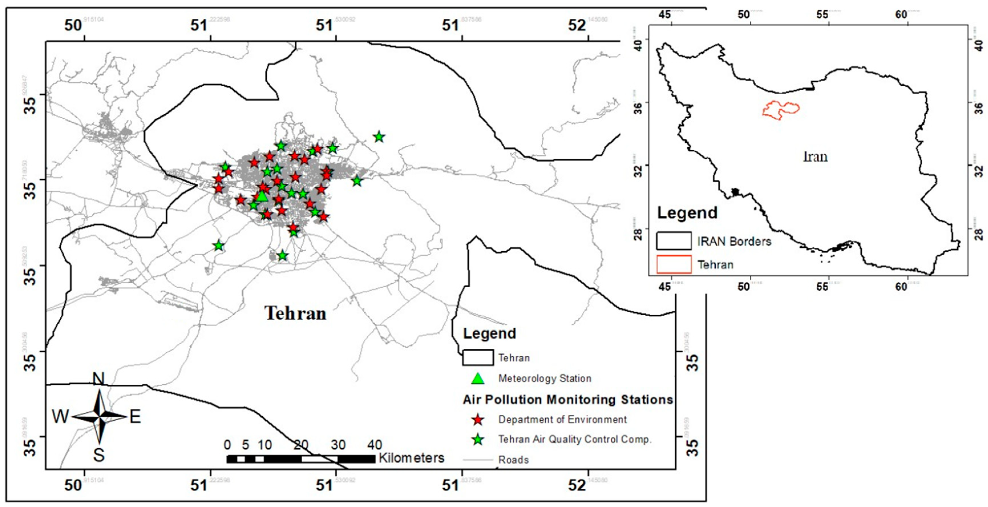
We focus on highly distributed air pollution monitoring (APM) sites in Tehran’s urban area. Missing values in Tehran’s ground-measured APM sites are a severe problem. In the urban area of Tehran, of 42 total APM sites, the rate of missing values in 11 of these for our study period is more than 75%. The difficulty with the missing data problem is also present in satellite-derived AODs, particularly AOD03 (96%) and AOD10 (63%). Nabavi et al. [
41] reported that that AOD retrieval algorithm based on a dark target considers the brightness of scenes as an indicator of the existence of aerosols. However, in urban areas, structures such as building roofs and streets act as bright surfaces, leading to miscalculation in AOD retrieval. It has been reported that 80% of AOD data from 2003 to 2017 was discarded because of this issue [
41]. In this work, Random Forest (RF), eXtreme Gradient Boosting (XGBoost), and Deep Neural Network (DNN) machine learning methods were used to investigate PM
2.5 concentration prediction. The performance of the predictions was evaluated using R
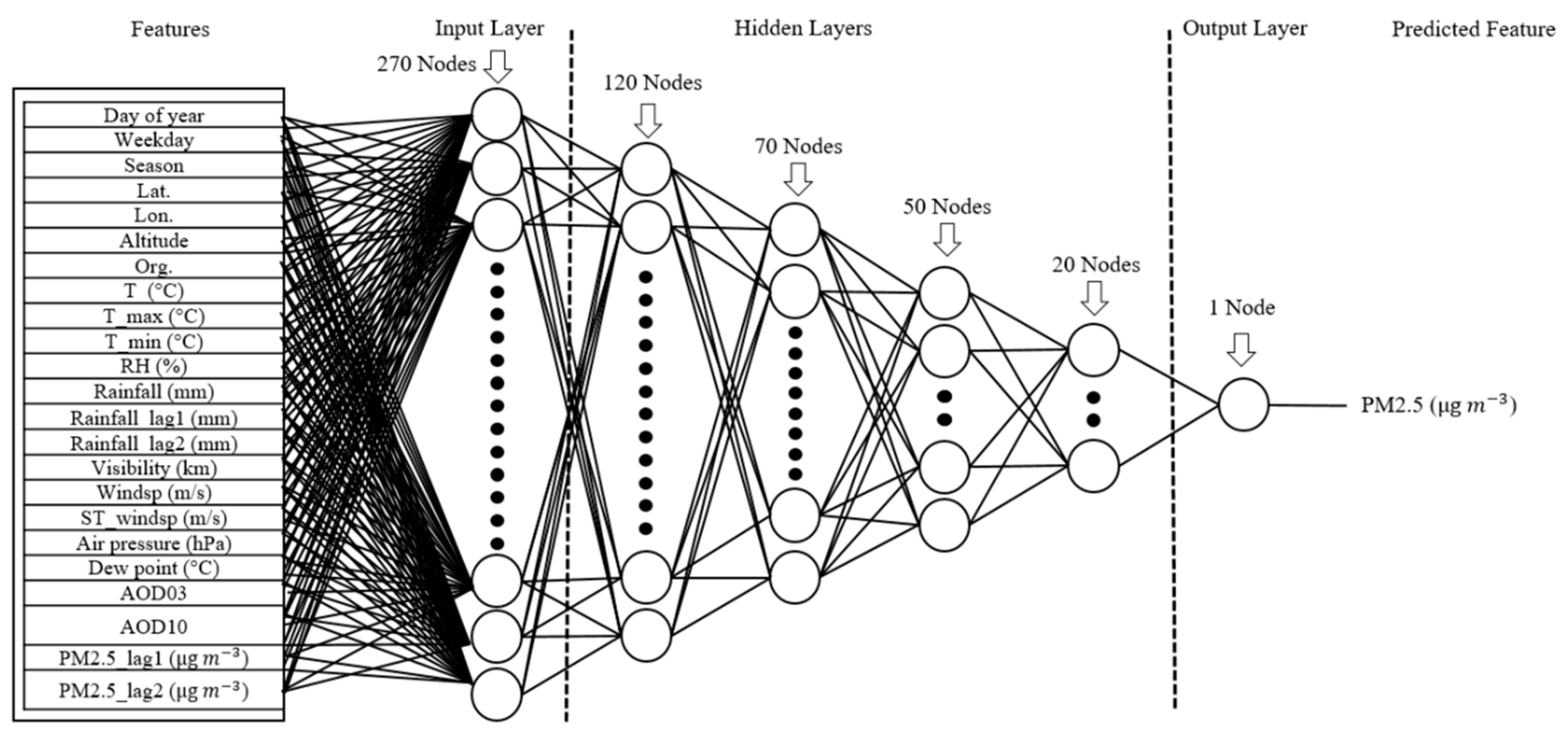
2, root mean square error (RMSE), and mean absolute error (MAE) metrics. A total of 23 features including AOD03, AOD10, meteorological data, geographic information of APM sites (latitude, longitude, and altitude), and other auxiliary features were used to predict PM
2.5. Finally, utilizing different methods, the importance of features for PM
2.5 concentration prediction was evaluated and compared. In addition, the most important features for PM
2.5 prediction were determined.
3. Results
Descriptive statistics of meteorological data and APM sites for the entire 4 year study period are illustrated in the
Supplementary Materials Section S3 and Tables S1 and S2. The missing value rate for most of the variables is less than 1.3% and for visibility only is 10.19%. The missing value for PM
2.5 was approximately 54.11%. This is caused by a critical failure of stations or power outage, maintenance, and so on [
17]. The AOD03 data show a high rate of missing values of approximately 94.09%. Thus, although there is an improvement in version 6.1 of the MODIS AOD product, it is not acceptable for this study area. The proportion of missing values in AOD10 is approximately 63.13%, which is better in comparison with AOD03. However, the product’s spatial resolution (10 km) is not high enough and multiple APM stations will share the same AOD value, while sampling the AOD10. The minimum and maximum altitude of APM stations are 1023 m and 1758 m above sea level. Five of the 42 APM stations have no instrument for PM
2.5 concentration measurement. The histograms of features are illustrated in
Section S4 Figure S1 of Supplementary Materials. The PM
2.5, AOD03, AOD10, windsp, and air_pressure histograms have an almost bell shaped distribution, while the other features show no special uniform distribution.
3.1. Model Performance Validation
In this study, we used AOD derived satellite data, in addition to ground measured climatic data and 37 APM stations, to predict the PM2.5 concentration. Three methods of machine learning—RF, XGBoost, and deep learning—were used for predictions. The dataset size has a significant impact on model training performance, particularly for the deep neural network. The AOD03 has a high rate of missing values (94%). Therefore, we conducted three tests, including AOD03 and excluding AOD03 and excluding both AODs, for each training. In addition, records with missing values were excluded from training and test datasets. All of the 1900 (including AOD03) and 11,800 (excluding AOD03) non-missing records out of a 41.2 k data size were used for training the models. The R2, MAE, and RMSE metrics were used to evaluate and compare the performance of the three methods.
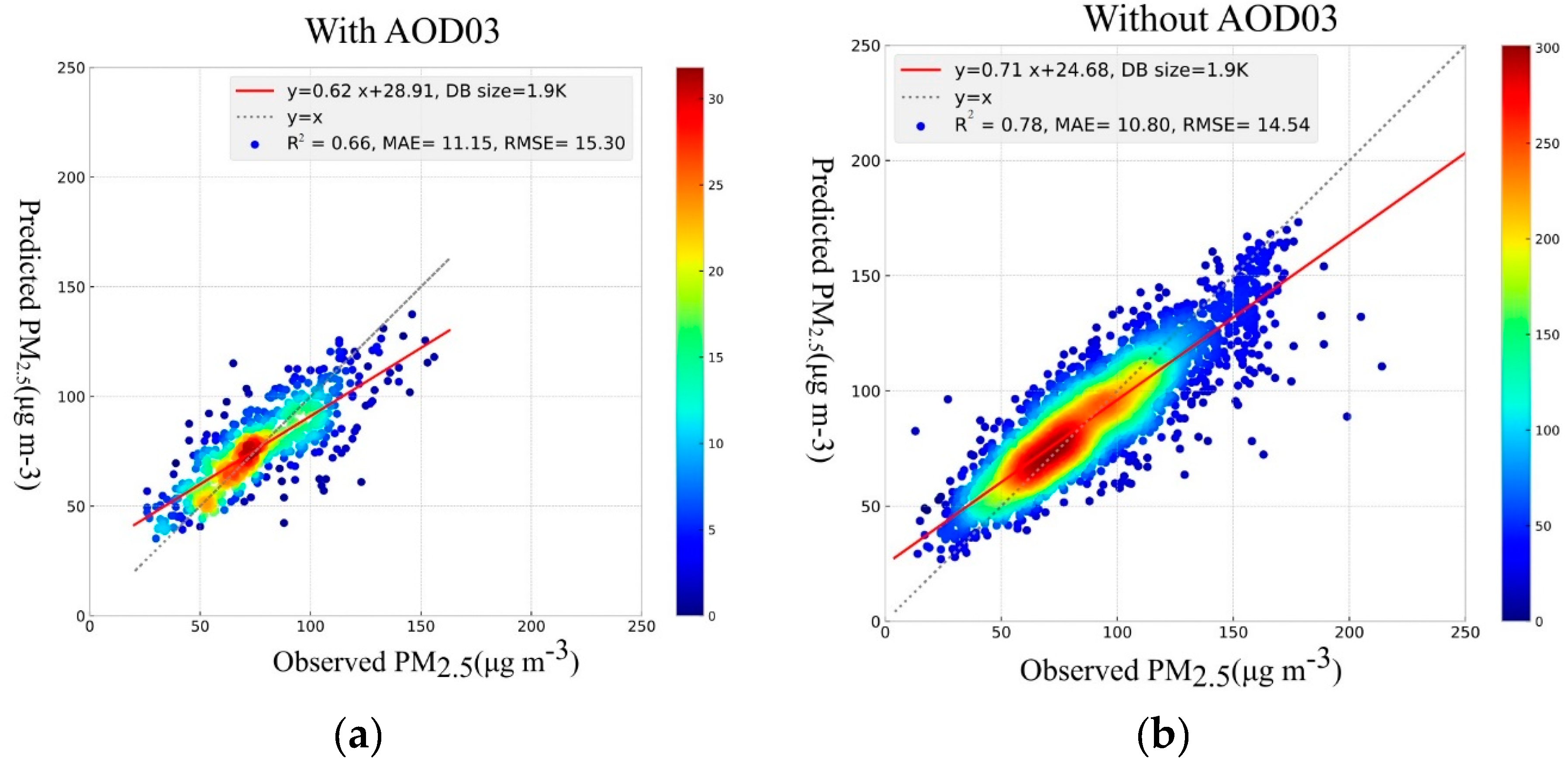
3.1.1. Random Forest
The optimum configuration of random forest modeling was obtained using the built-in grid search function in Python, with the 10-fold cross-validation technique. The optimum values are shown in
Table 2. For records size, the best performance is seen while excluding the AOD03 from the model input features. The prediction metrics show R
2 (R = 0.88), MAE = 10.8 µg/m
3, and RMSE = 14.54 µg/m
3. The predicted vs. observed scattered points are distributed around the y = x reference line and the density of points is closer to the reference line. This exhibits a reasonable prediction of PM
2.5 (see
Figure 3a,b). Excluding both AODs shows almost the same performance as a test with AOD10.
3.1.2. XGBoost
The scatter plot of predicted PM
2.5 versus observed values using the XGBoost method is illustrated in
Figure 4.
Figure 4a shows the scatterplot of predicted vs. observed PM
2.5 values considering all parameters.
Figure 4b shows the scatterplot of predicted vs. observed PM
2.5 values excluding the AOD03 variable. The scattered points are distributed around the y = x reference line, demonstrating a reasonable prediction of PM
2.5 concentration. Excluding both AODs shows the same performance as a test with AOD10.
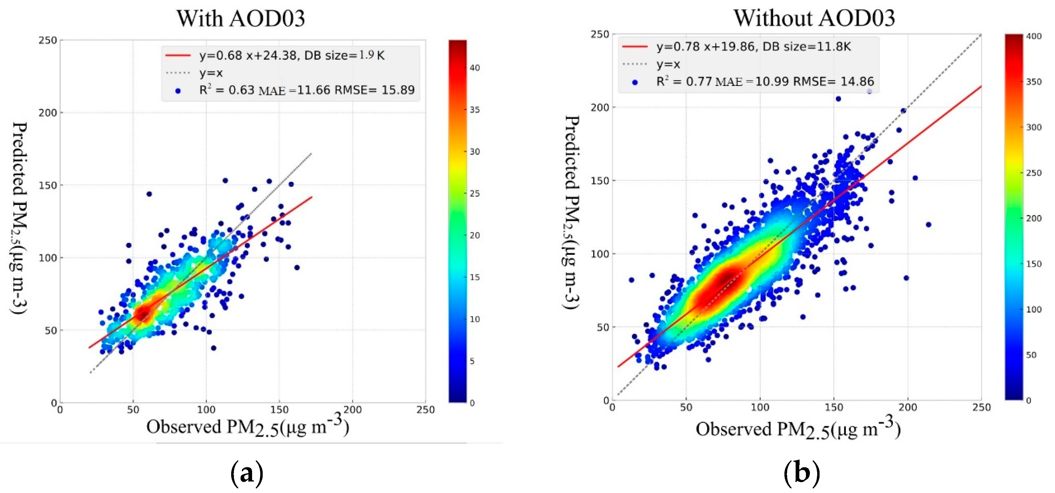
3.1.3. Deep Learning
Deep neural networks are very sensitive to the input features range and easily become unstable during the training process. In the first step, 1900 (including AOD03) and 11,800 (excluding AOD03) records were selected, based on non-missing records. Moreover, a standard scaler was used to normalize the features to (−1,1). The model was trained based on 70% of selected records that were shuffled in advance. The scatter plots of predicted PM
2.5 concentration versus observed values, considering all features, is illustrated in
Figure 5. The best model performance was achieved by excluding AOD03 from the input features, with R
2 = 0.77 (R = 0.88), MAE = 10.99 µg/m
3, and RMSE = 14.86 µg/m
3. Although the R
2 value obtained by deep learning is lower than for RF and XGBoost, the distribution of predictions vs. observed points around the y = x reference line still demonstrates acceptable performance. Excluding both AODs shows the same performance as a test with AOD10.
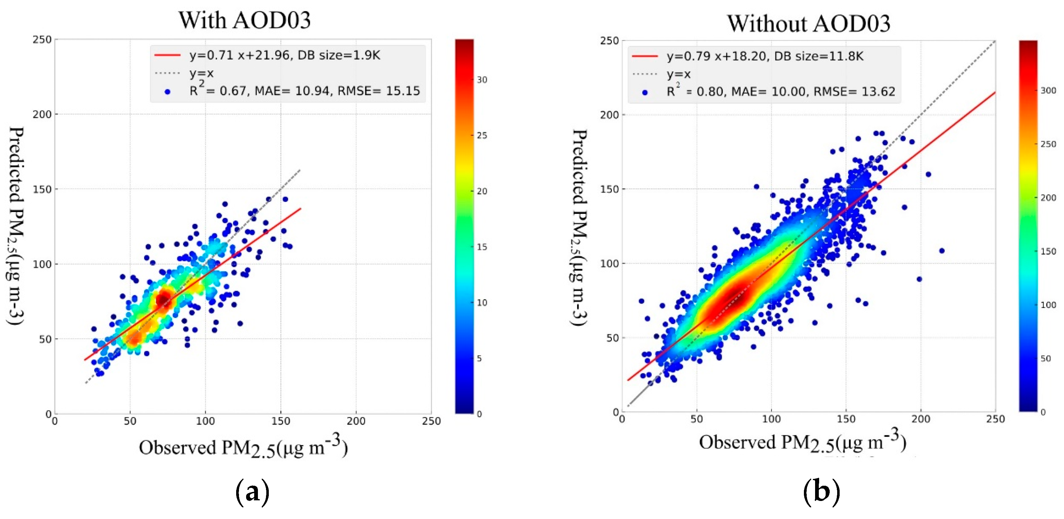
The results for all three modeling approaches with and without AOD03 and without both AODs, are shown in
Table 5. The XGBoost method demonstrates the highest model performance with R
2 = 0.8 (R = 0.894), MAE = 10.0 µg/m
3, and RMSE = 13.62 µg/m
3, while excluding the AOD03. This shows that AOD03 is not a good feature for PM
2.5 concentration prediction. In addition, excluding both AODs did not reduce the performance.
Therefore, it can be inferred that other features can act as a substitute for AODs. This decreases the importance of AODs on PM2.5 prediction. In addition, sample size has significant impact on modeling and prediction performance. Considering the performance metrics, all three ML methods demonstrate almost similar performance. The R2 values varied from 0.63 to 0.67, excluding AOD03, and 0.77 to 0.80 with AOD10 and without AODs. The best model performance was obtained with the XGBoost ML method, with a very low time cost of 19 s.
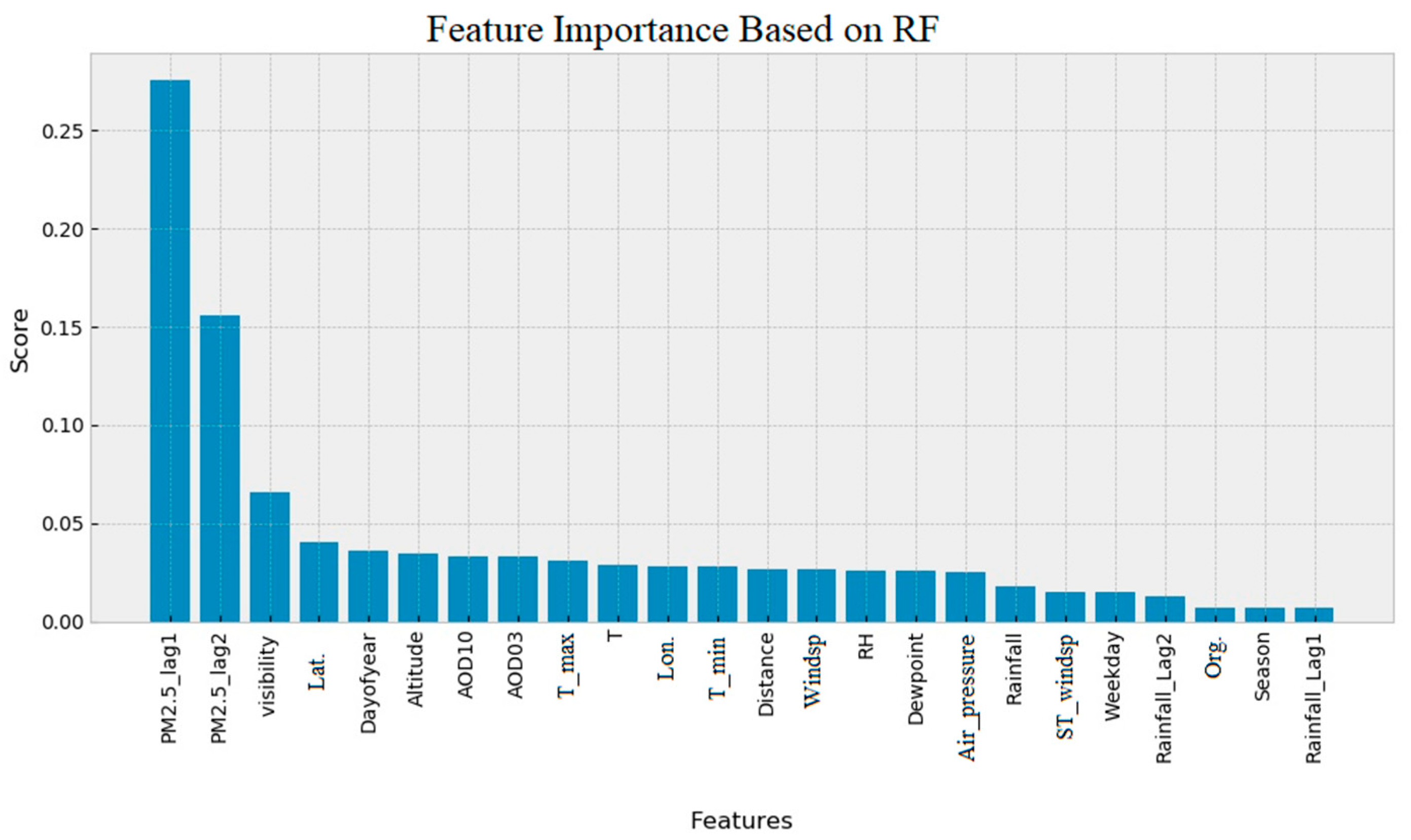
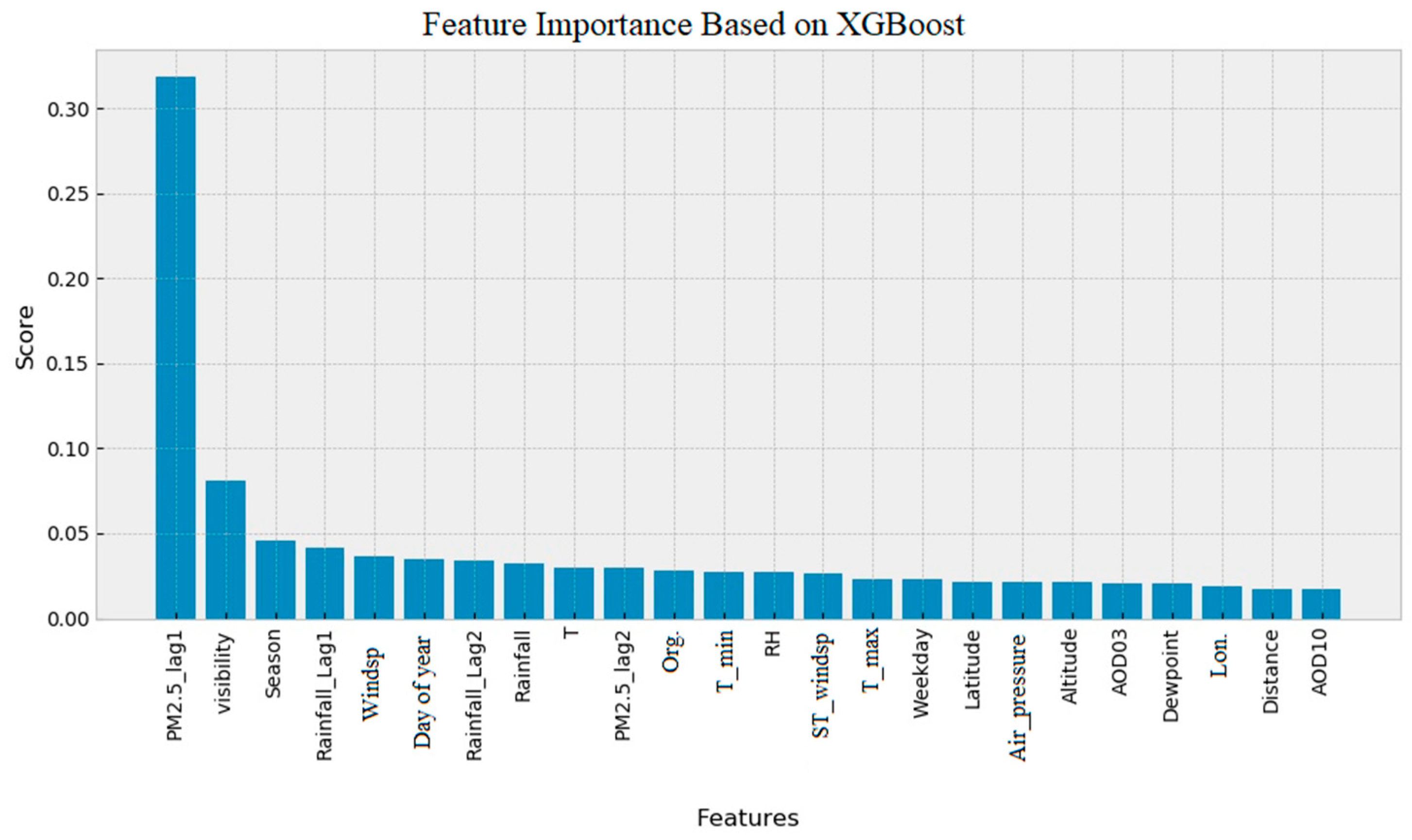
3.2. Feature Importance Assessment
3.2.1. RF and XGBoost Feature Importance Ranking
Some features do not contribute to the modeling and only increase the complexity of the model. Therefore, we conducted a feature importance assessment, to detect and eliminate useless features. The RF and XGBoost have a built-in function that evaluates the features importance. The feature importance bar graph plot based on RF and XGBoost modeling is shown in
Figure 6 and
Figure 7. The features are sorted based on their importance. In both RF and XGBoost, PM2.5_lag1 and visibility show significant importance compared to the other features.
However, there are large differences between RF and XGBoost feature importance ranking results. For example, AOD10 has the lowest rank in XGBoost feature ranking, while AOD10 is ranked seventh in the feature importance ranking by the RF method. Some studies have reported that the feature importance ranking built-in function of RF is biased and unreliable [
58] and suggest carrying out the features permutation for feature importance ranking.
3.2.2. Feature Permutation Using Deep Neural Network
The
Table 6 shows the feature permutation impact on the prediction performance of a well-trained DNN model. It is reasonable that by permuting an important feature, lower prediction performance be obtained.
Considering the feature importance ranking obtained by features permutation, we repeated DNN training 23 times. In round one, PM2.5_lag1 was used as the input feature and model performance was measured. In the second round of training, features with the rank of 1 and 2 were used as input features. This procedure was repeated to cover all 23 features. In each step, the R
2 value was measured to evaluate model performance. The best model performance during this procedure was obtained using the 15 most important features (from PM2.5_lag1 to dew point), with R
2 of 0.776. In the
Table 6 column “R
2 based on ranking”, the result of this procedure is presented, and less important features are marked with bold font. A negative effect on R
2 value was observed after adding more features. Therefore, the best DNN model performance using useless feature reduction is a R
2 of 0.776.
3.2.3. MAE Based Feature Elimination Using XGBoost
In addition to the other methods explained above, we conducted a recursive XGBoost training procedure, with feature removal based on MAE metrics. In the first step, a model was trained using all features and the performance of the model measured using MAE metrics. In the second step, the training was repeated 23 times, by removing one of the features at each round and measuring MAE metrics. In the third step, feature with the lowest effect on model performance (lowest MAE) was removed from the total features. The procedure was repeated using 22 features and so on until three features remained. The results are illustrated in
Figure 8.
These results demonstrate that removing RH in the first step improved the model. Model performance did not decrease when RH, longitude, T, sustained wind speed, distance, rainfall_lag2, T_min, org., and weekdays (located on the left side of the dashed blue line in
Figure 8 were removed. In addition, removing season, T_max, AOD10, and rainfall did not change the R
2 value and had a small effect on MAE and RMSE. Feature dependency may be the reason for the low changes in model performance. The best model performance obtained by this method was R
2 = 0.81.
4. Discussion
Using different methods for feature importance evaluation, we achieved slightly different results. However, in most of the methods, historical observations of PM
2.5, wind speed, visibility, day of the year, altitude, and temperature were very important in modeling. The features importance ranking based on different modeling approaches is presented in
Table 7. The rankings median value for each feature is presented in
Table 7. Features are sorted from top down, based on the median of feature importance rankings. Features such as latitude are important for RF and XGBoost, but rank lower in the deep learning features permutation method. This is because some features are dependent and can be replaced by other features.
The features used in this study can be divided into three categories. The first category is features that directly carry spatial information, such as latitude, longitude, and altitude. The second category is features that indirectly carry APM station spatial information, such as AOD10, AOD03, PM2.5_lag1, and PM2.5_lag2. The third category is the parameters that are shared for all stations, such as meteorological data and day of year, day of week, and sampling season.
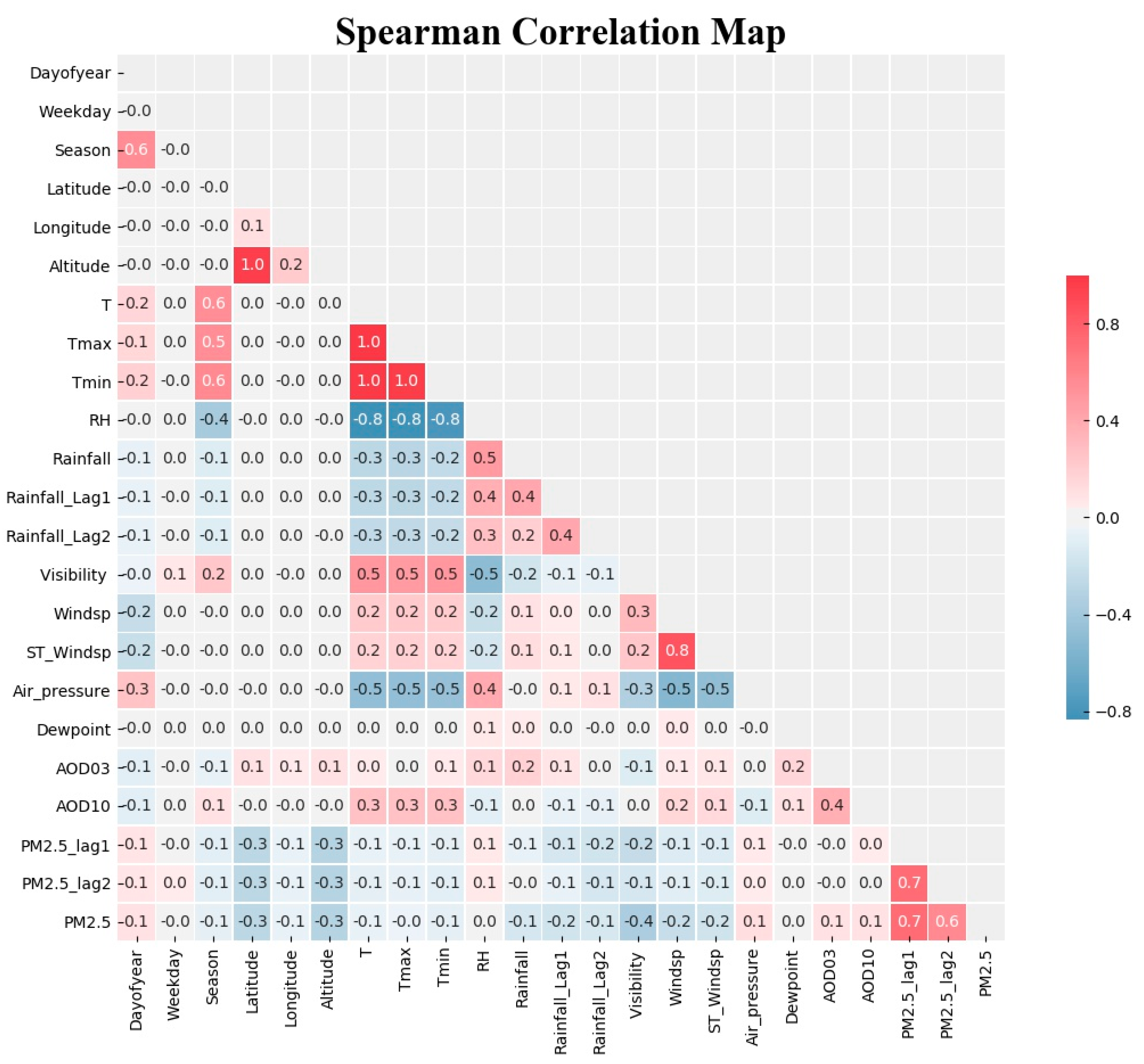
The Spearman’s correlation coefficient heat map of features is shown in
Figure 9. The PM
2.5 historical observation values have the highest correlation to PM
2.5. The air pressure, AOD03, and AOD10 have positive correlation with the PM
2.5. Visibility, wind speed, rainfall, altitude, and latitude show a negative correlation with the PM
2.5. Also, high correlation between other features reveals features dependency on each other. Dependent features can be predicted using other features, and subsequently can be eliminated from modeling to reduce the model complexity and cost of prediction.
Air temperature and pressure, dew point, and RH are dependent on altitude. We did not use the exact meteorological parameters for each station because of a lack of data; however, meteorological parameters can be modeled and predicted for each station based on altitude and other available features. Based on the Spearman correlation heat map, RH and air pressure are highly correlated with temperature. Considering the cost of prediction, they can be used as substitutes for each other. Some features such as temperature, RH, and pressure have a seasonal trend, and thus the feature “day of year” can facilitate modeling and improve the performance. Its ranking varies from 2 to 10 with a median value of 5.5.
In this study, three-machine learning techniques (RF, Deep learning, and XGBoost) were used to predict PM2.5 concentration. The XGBoost technique demonstrated the highest performance and an acceptable time of training. To detect features importance, permutation and recursive feature removal, in addition to RF and XGBoost built-in functions, were used. Some of differences in features importance ranking could be a result of features dependency. However, overall, the features rankings obtained in this paper are logical and beneficial for future studies.
5. Conclusions
In this study, we utilized Random forest, XGBoost, and Deep learning machine learning techniques to predict PM2.5 concentration in Tehran’s urban area. Widely distributed ground measured PM2.5 data, meteorological features, and remote sensing AOD data were used. In previous research, different methods and features were employed for PM2.5 concentration prediction. However, few studies dealt with the limitations of our study area, including the high rate of PM2.5 and AOD missing values. In addition, the air pollution monitoring sites in our study area were densely distributed, with just one available weather station. We also utilized 3 and 10 km MODIS AOD products, and geographic properties of the monitoring stations such as latitude, longitude, and topography. Also included were historical observation values of PM2.5 and rainfall, in addition to day of year, day of week, and season. Features importance and correlation were evaluated using the Spearman correlation method, permutation, recursive feature removal, and default built-in functions of the XGBoost and RFF techniques.
In comparison to RF and Deep learning methods, XGBoost achieved the best performance of approximately R
2 = 0.81 (R = 0.9), MAE = 09.92 µg/m
3, and RMSE = 13.58 µg/m
3, with very low cost of time (19 s). Although a DNN model was used for modeling and prediction, XGBoost with its simple structure, performed better. However, all three ML methods performed similarly and R
2 varied from 0.63 to 0.67, when Aerosol Optical Depth (AOD) at 3 km resolution was included, and 0.77 to 0.81, when AOD at 3 km resolution was excluded. Based on feature importance ranking, we found that there are features with high dependency on other features. Therefore, some features can be ranked differently based on machine learning structure. We investigated 23 features and determined that by using eight to 12 features, we can achieve acceptable PM
2.5 prediction performance. For example, with MAE based XGBoost feature removal, by using only nine of the most important features, such as PM2.5_lag1, day of year, wind speed, visibility, latitude, air pressure, dew point, PM2.5_lag2, and altitude (see
Figure 8), an acceptable performance of R
2 = 0.79 (R = 0.888), MAE = 10.20 µg/m
3, and RMSE = 14 µg/m
3 was obtained.
Most notably, this is the first study, to our knowledge, to investigate the importance of features for PM2.5 concentration prediction. New features such as latitude, longitude, altitude, and dew point, in addition to day of year, day of week, and season were utilized in a way that has not been done in previous work. However, some limitations are worth noting. Although we have achieved reasonable PM2.5 prediction performance, satellite-derived AODs did not have a significant impact on predictions. Yet, historical values of PM2.5 are necessary for reasonable PM2.5 prediction. In particular, AOD03 has a very high rate of missing values. Thus, it is not useful for our study area. Spatial distribution pattern prediction of PM2.5 is limited without historical values of PM2.5. Future work will focus on images with high spatial resolution, based on the important features introduced in this research.

 ,
, 


