Spatial Distributions and Sources of Inorganic Chlorine in PM2.5 across China in Winter

 ,
,
Abstract
:1. Introduction
2. Materials and Methods
2.1. Sampling and Chemical Analysis
2.2. Model of Positive Matrix Factorization
3. Results and Discussions
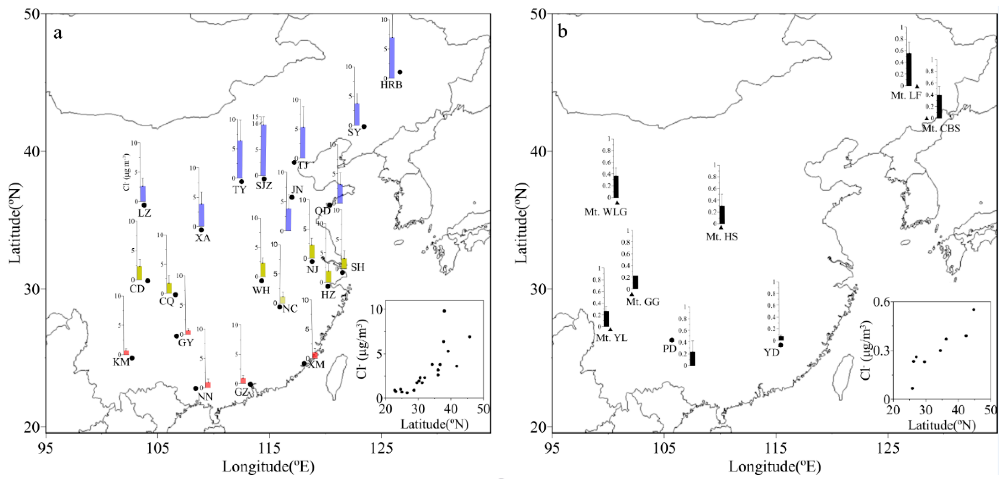
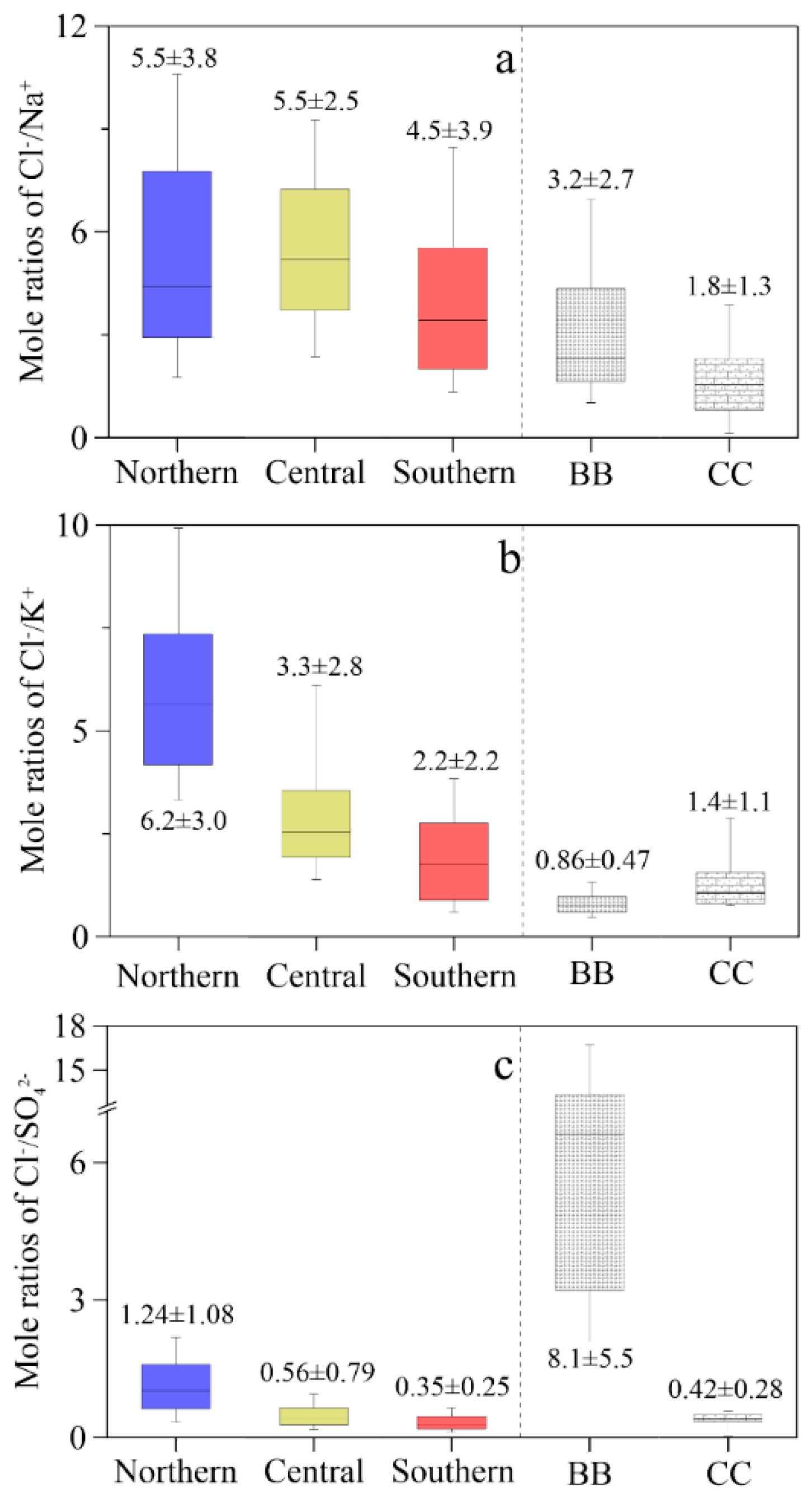
3.1. Spatial Distributions of Cl−, , K+ and Na+ in PM2.5
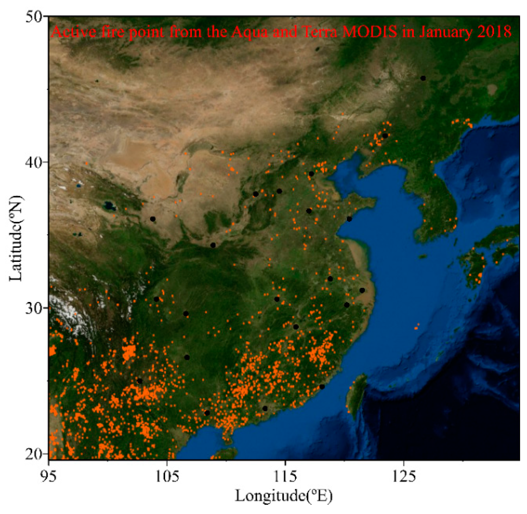
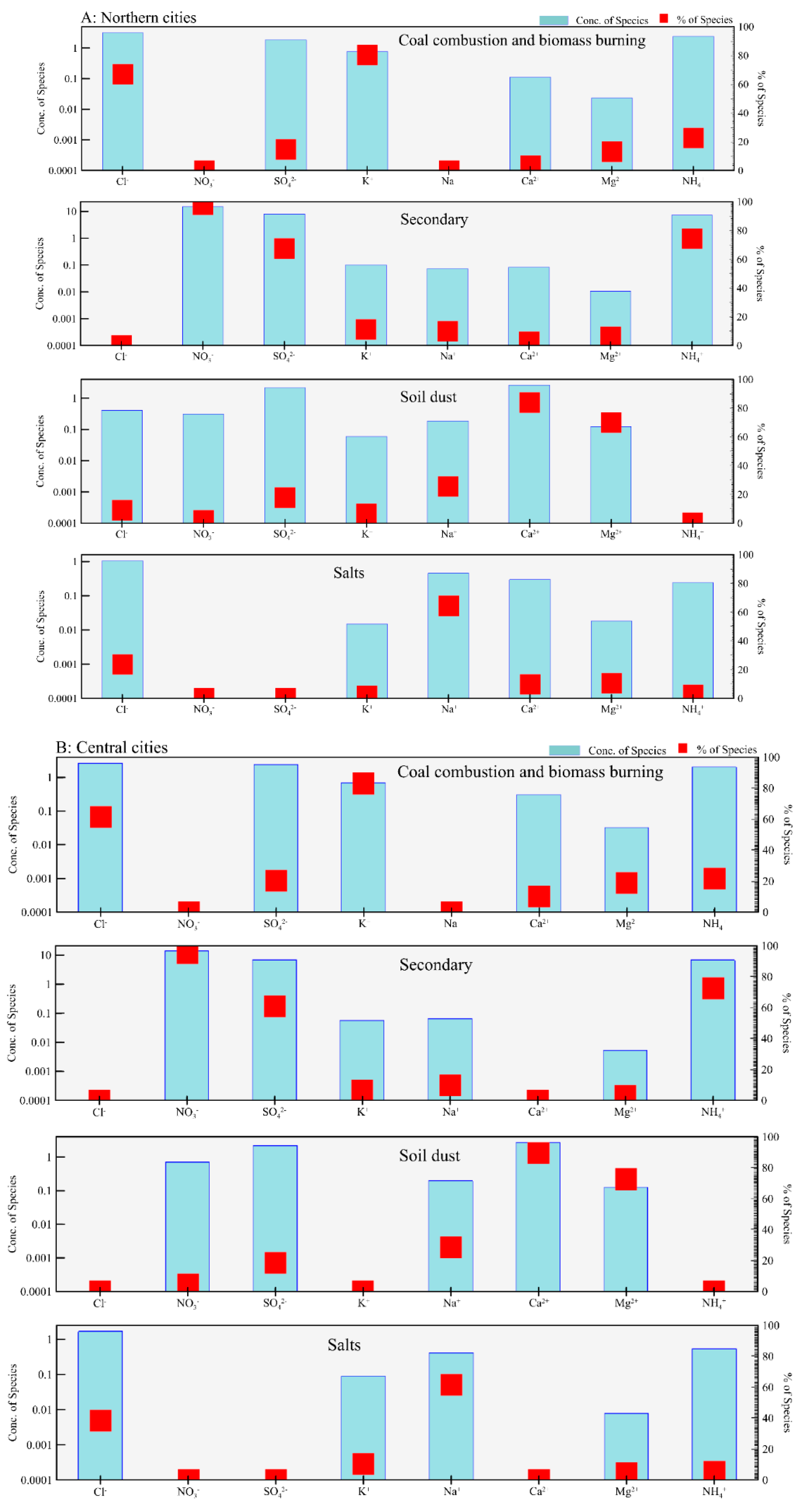
3.2. Source Apportionment of Cl− in PM2.5
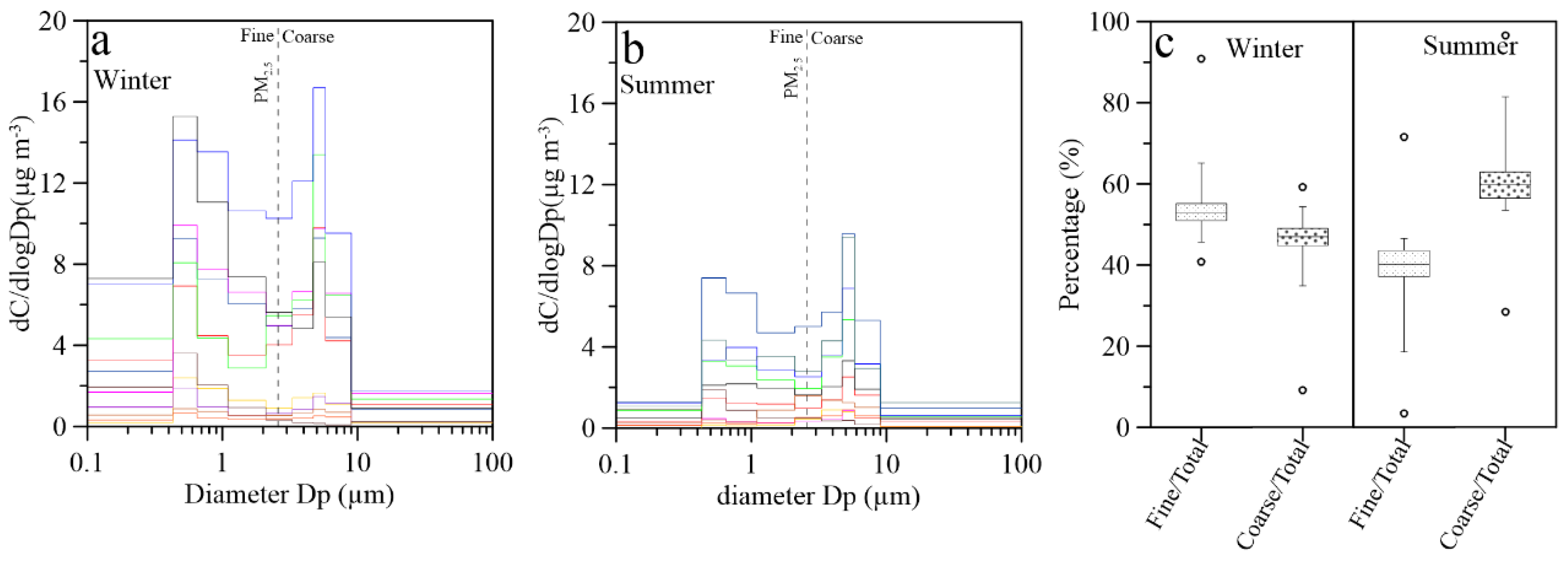
3.3. Size Distributions of Aerosol Cl−: A Review
4. Conclusions
Author Contributions
Funding
Conflicts of Interest
References
- Seinfeld, J.H.; Pandis, S.N. Atmospheric Chemistry and Physics: From Air Pollution to Climate Change, 2nd ed.; John Wiley & Sons, Inc.: New York, NY, USA, 2016. [Google Scholar]
- IPCC. Climate Change 2013: The Physical Science Basis; Cambridge University Press: Cambridge, UK, 2013. [Google Scholar]
- Hönninger, G.; Platt, U. Observations of BrO and its vertical distribution during surface ozone depletion at Alert. Atmos. Environ. 2002, 36, 2481–2489. [Google Scholar] [CrossRef]
- Sarwar, G.; Gantt, B.; Schwede, D.; Foley, K.; Mathur, R.; Saiz-Lopez, A. Impact of Enhanced Ozone Deposition and Halogen Chemistry on Tropospheric Ozone over the Northern Hemisphere. Environ. Sci. Technol. 2015, 49, 9203–9211. [Google Scholar] [CrossRef] [PubMed] [Green Version]
- Simpson, W.R.; Von Glasow, R.; Riedel, K.; Anderson, P.; Ariya, P.; Bottenheim, J.; Burrows, J.; Carpenter, L.J.; Fries, U.; Goodsite, M.E.; et al. Halogens and their role in polar boundary-layer ozone depletion. Atmos. Chem. Phys. 2007, 7, 4375–4418. [Google Scholar] [CrossRef] [Green Version]
- Saiz-Lopez, A.; Von Glasow, R. Reactive halogen chemistry in the troposphere. Chem. Soc. Rev. 2012, 41, 6448–6472. [Google Scholar] [CrossRef] [PubMed]
- Sherwen, T.; Schmidt, J.A.; Evans, M.J.; Carpenter, L.J.; Großmann, K.; Eastham, S.D.; Jacob, D.J.; Dix, B.; Koenig, T.K.; Sinreich, R.; et al. Global impacts of tropospheric halogens (Cl, Br, I) on oxidants and composition in GEOS-Chem. Atmos. Chem. Phys. 2016, 16, 12239–12271. [Google Scholar] [CrossRef] [Green Version]
- Ahern, A.T.; Goldberger, L.; Jahl, L.; Thornton, J.; Sullivan, R.C. Production of N2O5 and ClNO2 through Nocturnal Processing of Biomass-Burning Aerosol. Environ. Sci. Technol. 2018, 52, 550–559. [Google Scholar] [CrossRef] [PubMed]
- Morin, S.; Savarino, J.; Frey, M.M.; Yan, N.; Bekki, S.; Bottenheim, J.W.; Martins, J.M.F. Tracing the Origin and Fate of NOx in the Arctic Atmosphere Using Stable Isotopes in Nitrate. Science 2008, 322, 730–732. [Google Scholar] [CrossRef] [PubMed]
- Altieri, K.E.; Hastings, M.G.; Gobel, A.R.; Peters, A.J.; Sigman, D.M. Isotopic composition of rainwater nitrate at Bermuda: The influence of air mass source and chemistry in the marine boundary layer. J. Geophys. Res. Atmos. 2013, 118, 11304–11316. [Google Scholar] [CrossRef]
- Keene, W.C.; Savoie, D.L. The pH of deliquesced sea-salt aerosol in polluted marine air. Geophys. Res. Lett. 1998, 25, 2181–2184. [Google Scholar] [CrossRef]
- Von Glasow, R.; Sander, R. Variation of sea salt aerosol pH with relative humidity. Geophys. Res. Lett. 2001, 28, 247–250. [Google Scholar] [CrossRef] [Green Version]
- Zhao, Y.; Gao, Y. Acidic species and chloride depletion in coarse aerosol particles in the US east coast. Sci. Total Environ. 2008, 407, 541–547. [Google Scholar] [CrossRef]
- Haskins, J.D.; Jaeglé, L.; Shah, V.; Lee, B.H.; Lopez-Hilfiker, F.D.; Campuzano-Jost, P.; Schroder, J.C.; Day, D.A.; Guo, H.; Sullivan, A.P.; et al. Wintertime Gas-Particle Partitioning and Speciation of Inorganic Chlorine in the Lower Troposphere Over the Northeast United States and Coastal Ocean. J. Geophys. Res. Atmos. 2018, 123, 12897–12916. [Google Scholar] [CrossRef]
- Sasakawa, M.; Uematsu, M. Relative contribution of chemical composition to acidification of sea fog (stratus) over the northern North Pacific and its marginal seas. Atmos. Environ. 2005, 39, 1357–1362. [Google Scholar] [CrossRef]
- Luo, L.; Yao, X.H.; Gao, H.W.; Hsu, S.C.; Li, J.W.; Kao, S.J. Nitrogen speciation in various types of aerosols in spring over the northwestern Pacific Ocean. Atmos. Chem. Phys. 2016, 16, 325–341. [Google Scholar] [CrossRef] [Green Version]
- Volpe, C.; Spivack, A.J.; Wahlen, M.; Pszenny, A.A.P. Chlorine isotopic composition of marine aerosols: Implications for the release of reactive chlorine and HCl cycling rates. Geophys. Res. Lett. 1998, 25, 3831–3834. [Google Scholar] [CrossRef]
- Koehler, G.; Wassenaar, L.I. The stable isotopic composition (37Cl/35Cl) of dissolved chloride in rainwater. Appl. Geochem. 2010, 25, 91–96. [Google Scholar] [CrossRef]
- Keene, W.C.; Khalil, M.A.K.; Erickson, D.J.; McCulloch, A.; Graedel, T.E.; Lobert, J.M.; Aucott, M.L.; Gong, S.L.; Harper, D.B.; Kleiman, G.; et al. Composite global emissions of reactive chlorine from anthropogenic and natural sources: Reactive Chlorine Emissions Inventory. J. Geophys. Res. Space Phys. 1999, 104, 8429–8440. [Google Scholar] [CrossRef] [Green Version]
- Zhang, R.; Jing, J.; Tao, J.; Hsu, S.-C.; Wang, G.; Cao, J.; Lee, C.S.L.; Zhu, L.; Chen, Z.; Zhao, Y. Chemical characterization and source apportionment of PM2.5 in Beijing: Seasonal perspective. Atmos. Chem. Phys. 2013, 13, 7053–7074. [Google Scholar] [CrossRef]
- Christian, T.J.; Yokelson, R.J.; Cárdenas, B.; Molina, L.T.; Engling, G.; Hsu, S.-C. Trace gas and particle emissions from domestic and industrial biofuel use and garbage burning in central Mexico. Atmos. Chem. Phys. 2010, 10, 565–584. [Google Scholar] [CrossRef] [Green Version]
- Luo, L.; Wu, Y.; Xiao, H.; Zhang, R.; Lin, H.; Zhang, X.; Kao, S.-J. Origins of aerosol nitrate in Beijing during late winter through spring. Sci. Total Environ. 2019, 653, 776–782. [Google Scholar] [CrossRef]
- Seuzaret, C.; Gong, S.L.; Erickson, D.J.; Keene, W.C. A general circulation model based calculation of HCl and ClNO2 production from sea salt dechlorination: Reactive Chlorine Emissions Inventory. J. Geophys. Res. Space Phys. 1999, 104, 8347–8372. [Google Scholar] [CrossRef]
- Lobert, J.M.; Yevich, R.; Keene, W.C.; Logan, J.A. Global chlorine emissions from biomass burning: Reactive Chlorine Emissions Inventory. J. Geophys. Res. Space Phys. 1999, 104, 8373–8389. [Google Scholar] [CrossRef] [Green Version]
- Liss, P.S.; Johnson, M.T. Ocean-Atmosphere Interactions of Gases and Particles; Springer: Heidelberg, Germany; New York, NY, USA; Dordrecht, Netherlands; London, UK, 2014. [Google Scholar]
- Zhang, X.; Zhuang, G.; Yuan, H.; Rahn, K.A.; Wang, Z.; An, Z. Aerosol Particles from Dried Salt-Lakes and Saline Soils Carried on Dust Storms over Beijing. Terr. Atmos. Ocean. Sci. 2009, 20, 6. [Google Scholar] [CrossRef]
- Delmelle, P.; Stix, J.; Bourque, C.P.-A.; Baxter, P.J.; Garcia-Alvarez, J.; Barquero, J. Dry Deposition and Heavy Acid Loading in the Vicinity of Masaya Volcano, a Major Sulfur and Chlorine Source in Nicaragua. Environ. Sci. Technol. 2001, 35, 1289–1293. [Google Scholar] [CrossRef] [PubMed]
- Stewart, M.A.; Spivack, A.J. The Stable-Chlorine Isotope Compositions of Natural and Anthropogenic Materials. Rev. Miner. Geochem. 2004, 55, 231–254. [Google Scholar] [CrossRef]
- Wang, H.; Zhuang, Y.; Wang, Y.; Sun, Y.; Yuan, H.; Zhuang, G.; Hao, Z. Long-term monitoring and source apportionment of PM2.5/PM10 in Beijing, China. J. Environ. Sci. 2008, 20, 1323–1327. [Google Scholar] [CrossRef]
- Galon-Negru, A.G.; Olariu, R.I.; Arsene, C. Chemical characteristics of size-resolved atmospheric aerosols in Iasi, north-eastern Romania: Nitrogen-containing inorganic compounds control aerosol chemistry in the area. Atmos. Chem. Phys. 2018, 18, 5879–5904. [Google Scholar] [CrossRef]
- Arsene, C.; Olariu, R.I.; Zarmpas, P.; Kanakidou, M.; Mihalopoulos, N. Ion composition of coarse and fine particles in Iasi, north-eastern Romania: Implications for aerosols chemistry in the area. Atmos. Environ. 2011, 45, 906–916. [Google Scholar] [CrossRef]
- Yokelson, R.J.; Burling, I.R.; Urbanski, S.P.; Atlas, E.L.; Adachi, K.; Buseck, P.R.; Wiedinmyer, C.; Akagi, S.K.; Toohey, D.W.; Wold, C.E.; et al. Trace gas and particle emissions from open biomass burning in Mexico. Atmos. Chem. Phys. 2011, 11, 6787–6808. [Google Scholar] [CrossRef] [Green Version]
- Cheng, Y.; Engling, G.; He, K.-B.; Duan, F.-K.; Ma, Y.-L.; Du, Z.-Y.; Liu, J.-M.; Zheng, M.; Weber, R.J. Biomass burning contribution to Beijing aerosol. Atmos. Chem. Phys. 2013, 13, 7765–7781. [Google Scholar] [CrossRef] [Green Version]
- Zhang, J.; Cheng, M.; Ji, D.; Liu, Z.; Hu, B.; Sun, Y.; Wang, Y. Characterization of submicron particles during biomass burning and coal combustion periods in Beijing, China. Sci. Total Environ. 2016, 562, 812–821. [Google Scholar] [CrossRef] [PubMed]
- Sun, Y.; Jiang, Q.; Xu, Y.; Ma, Y.; Zhang, Y.; Liu, X.; Li, W.; Wang, F. Aerosol characterization over the North China Plain: Haze life cycle and biomass burning impacts in summer. J. Geophys. Res. Atmos. 2016, 121, 2508–2521. [Google Scholar] [CrossRef] [Green Version]
- Duce, R.A.; Laroche, J.; Altieri, K.; Arrigo, K.R.; Baker, A.R.; Capone, D.G.; Cornell, S.; Dentener, F.; Galloway, J.; Ganeshram, R.S.; et al. Impacts of Atmospheric Anthropogenic Nitrogen on the Open Ocean. Science 2008, 320, 893–897. [Google Scholar] [CrossRef] [PubMed] [Green Version]
- Kim, T.-W.; Lee, K.; Najjar, R.G.; Jeong, H.-D.; Jeong, H.J. Increasing N Abundance in the Northwestern Pacific Ocean Due to Atmospheric Nitrogen Deposition. Science 2011, 334, 505–509. [Google Scholar] [CrossRef] [PubMed] [Green Version]
- Liu, X.; Zhang, Y.; Han, W.; Tang, A.; Shen, J.; Cui, Z.; Vitousek, P.; Erisman, J.W.; Goulding, K.; Christie, P.; et al. Enhanced nitrogen deposition over China. Nature 2013, 494, 459–462. [Google Scholar] [CrossRef] [PubMed]
- Elser, J.J.; Andersen, T.; Baron, J.S.; Bergström, A.-K.; Jansson, M.; Kyle, M.; Nydick, K.R.; Steger, L.; Hessen, D.O. Shifts in Lake N:P Stoichiometry and Nutrient Limitation Driven by Atmospheric Nitrogen Deposition. Science 2009, 326, 835–837. [Google Scholar] [CrossRef] [PubMed]
- Lovett, G.M.; Likens, G.E.; Buso, D.C.; Driscoll, C.T.; Bailey, S.W. The biogeochemistry of chlorine at Hubbard brook, New Hampshire, USA. Biogeochemistry 2005, 72, 191–232. [Google Scholar] [CrossRef]
- Alcalá, F.J.; Custodio, E.; Alcala, F. Atmospheric chloride deposition in continental Spain. Hydrol. Process. 2008, 22, 3636–3650. [Google Scholar] [CrossRef]
- Orehova, T.; Vasileva, T. Evaluation of the atmospheric chloride deposition in the Danube hydrological zone of Bulgaria. Environ. Earth Sci. 2014, 72, 1143–1154. [Google Scholar] [CrossRef]
- Davies, P.; Crosbie, R. Mapping the spatial distribution of chloride deposition across Australia. J. Hydrol. 2018, 561, 76–88. [Google Scholar] [CrossRef]
- Kubzova, M.; Krivy, V.; Kreislova, K. Influence of Chloride Deposition on Corrosion Products. Procedia Eng. 2017, 192, 504–509. [Google Scholar] [CrossRef]
- De la Fuente, D.; Díaz, I.; Alcántara, J.; Chico, B.; Simancas, J.; Llorente, I.; García-Delgado, A.; Jiménez, J.A.; Adeva, P.; Morcillo, M. Corrosion mechanisms of mild steel in chloride-rich atmospheres. Mater. Corros. 2016, 67, 227–238. [Google Scholar] [CrossRef]
- Ma, Y.; Li, Y.; Wang, F. Corrosion of low carbon steel in atmospheric environments of different chloride content. Corros. Sci. 2009, 51, 997–1006. [Google Scholar] [CrossRef]
- Dong, J.; Han, E.; Ke, W. Introduction to atmospheric corrosion research in China. Sci. Technol. Adv. Mater. 2007, 8, 559–565. [Google Scholar] [CrossRef] [Green Version]
- Hsu, S.-C.; Gong, G.-C.; Shiah, F.-K.; Hung, C.-C.; Kao, S.-J.; Zhang, R.; Chen, W.-N.; Chen, C.-C.; Chou, C.C.-K.; Lin, Y.-C.; et al. Sources, solubility, and acid processing of aerosol iron and phosphorous over the South China Sea: East Asian dust and pollution outflows vs. Southeast Asian biomass burning. Atmos. Chem. Phys. Discuss. 2014, 14, 21433–21472. [Google Scholar] [CrossRef] [Green Version]
- Norris, G.; Duvall, R. Positive Matrix Factorization (PMF) 5.0 Fundamentals & User Guide; U.S. Environmental Protection Agency: Washington, DC, USA, 2014.
- Zhou, L.; Kim, E.; Hopke, P.K.; Stanier, C.; Pandis, S. Mining airborne particulate size distribution data by positive matrix factorization. J. Geophys. Res. Space Phys. 2005, 110. [Google Scholar] [CrossRef] [Green Version]
- Zhang, Y.; Sheesley, R.J.; Schauer, J.J.; Lewandowski, M.; Jaoui, M.; Offenberg, J.H.; Kleindienst, T.E.; Edney, E.O. Source apportionment of primary and secondary organic aerosols using positive matrix factorization (PMF) of molecular markers. Atmos. Environ. 2009, 43, 5567–5574. [Google Scholar] [CrossRef]
- Yang, Y.; Zhou, R.; Wu, J.; Yu, Y.; Ma, Z.; Zhang, L.; Di, Y. Seasonal variations and size distributions of water-soluble ions in atmospheric aerosols in Beijing, 2012. J. Environ. Sci. 2015, 34, 197–205. [Google Scholar] [CrossRef]
- Cao, J.-J.; Shen, Z.-X.; Chow, J.C.; Watson, J.G.; Lee, S.-C.; Tie, X.-X.; Ho, K.-F.; Wang, G.-H.; Han, Y.-M. Winter and summer PM2.5 chemical compositions in fourteen Chinese cities. J. Air Waste Manag. Assoc. 2012, 62, 1214–1226. [Google Scholar] [CrossRef]
- Huang, R.-J.; Zhang, Y.; Bozzetti, C.; Ho, K.-F.; Cao, J.-J.; Han, Y.; Daellenbach, K.R.; Slowik, J.G.; Platt, S.M.; Canonaco, F.; et al. High secondary aerosol contribution to particulate pollution during haze events in China. Nature 2014, 514, 218–222. [Google Scholar] [CrossRef] [Green Version]
- Ji, D.; Li, L.; Wang, Y.; Zhang, J.; Cheng, M.; Sun, Y.; Liu, Z.; Wang, L.; Tang, G.; Hu, B.; et al. The heaviest particulate air-pollution episodes occurred in northern China in January, 2013: Insights gained from observation. Atmos. Environ. 2014, 92, 546–556. [Google Scholar] [CrossRef]
- Vieira-Filho, M.; Pedrotti, J.J.; Fornaro, A. Water-soluble ions species of size-resolved aerosols: Implications for the atmospheric acidity in São Paulo megacity, Brazil. Atmos. Res. 2016, 181, 281–287. [Google Scholar] [CrossRef]
- Liu, Y.; Fan, Q.; Chen, X.; Zhao, J.; Ling, Z.; Hong, Y.; Li, W.; Chen, X.; Wang, M.; Wei, X. Modeling the impact of chlorine emissions from coal combustion and prescribed waste incineration on tropospheric ozone formation in China. Atmos. Chem. Phys. 2018, 18, 2709–2724. [Google Scholar] [CrossRef] [Green Version]
- Yang, X.; Wang, T.; Xia, M.; Gao, X.; Li, Q.; Zhang, N.; Gao, Y.; Lee, S.; Wang, X.; Xue, L.; et al. Abundance and origin of fine particulate chloride in continental China. Sci. Total Environ. 2018, 624, 1041–1051. [Google Scholar] [CrossRef] [PubMed]
- Li, J.; Wang, G.; Zhou, B.; Cheng, C.; Cao, J.; Shen, Z.; An, Z. Chemical composition and size distribution of wintertime aerosols in the atmosphere of Mt. Hua in central China. Atmos. Environ. 2011, 45, 1251–1258. [Google Scholar] [CrossRef]
- Zhang, N.; Cao, J.; Ho, K.; He, Y. Chemical characterization of aerosol collected at Mt. Yulong in wintertime on the southeastern Tibetan Plateau. Atmos. Res. 2012, 107, 76–85. [Google Scholar] [CrossRef]
- Zhao, Y.-N.; Wang, Y.-S.; Wen, T.-X.; Yang, Y.-J.; Li, W. Observation and analysis on water-soluble inorganic chemical compositions of atmospheric aerosol in Gongga Mountain. Huan Jing Ke Xue 2009, 30, 9–13. [Google Scholar]
- Zhao, Y.-N.; Wang, Y.-S.; Wen, T.-X.; Dai, G.-H. Seasonal variation of water-soluble ions in PM2.5 at Changbai Mountain. Huan Jing Ke Xue 2014, 35, 9–14. [Google Scholar]
- Yang, D.; Yu, X.; Fang, X.; Wu, F.; Li, X. A study of aerosol at regional background stations and baseline station. Q. J. Appl. Meteorol. 1996, 7, 396–405. [Google Scholar]
- Hsu, S.C.; Liu, S.C.; Huang, Y.T.; Chou, C.C.K.; Lung, S.C.C.; Liu, T.H.; Tu, J.Y.; Tsai, F. Long-range southeastward transport of asian biosmoke pollution: Signature detected by aerosol potassium in northern taiwan-article no. d14301. J. Geophys. Res. Atmos. 2019, 114. [Google Scholar] [CrossRef]
- Weber, R.J.; Lee, Y.; Orsini, D.A.; Maxwell-Meier, K.; Thornton, D.C.; Bandy, A.R.; Clarke, A.D.; Sachse, G.W.; Fuelberg, H.E.; Kiley, C.M.; et al. Characteristics and influence of biosmoke on the fine-particle ionic composition measured in Asian outflow during the Transport and Chemical Evolution Over the Pacific (TRACE-P) experiment. J. Geophys. Res. Space Phys. 2003, 108, 8816. [Google Scholar] [CrossRef]
- Waldman, J.; Lioy, P.; Zelenka, M.; Jing, L.; Lin, Y.; He, Q.; Qian, Z.; Chapman, R.; Wilson, W. Wintertime measurements of aerosol acidity and trace elements in Wuhan, a city in central China. Atmos. Environ. Part B Urban Atmos. 1991, 25, 113–120. [Google Scholar] [CrossRef]
- Xu, Y.; Liu, X.; Zhang, P.; Guo, J.; Han, J.; Zhou, Z.; Xu, M. Role of chlorine in ultrafine particulate matter formation during the combustion of a blend of high-Cl coal and low-Cl coal. Fuel 2016, 184, 185–191. [Google Scholar] [CrossRef]
- Yan, Q.; Kong, S.; Liu, H.; Wang, W.; Wu, J.; Zheng, M.; Zheng, S.; Yang, G.; Wu, F. Emission inventory of water soluble ions in fine particles from residential coal burning in China and implication for emission reduction. China Environ. Sci. 2017, 37, 3708–3721. (In Chinese) [Google Scholar]
- Chester, R. Marine Geochemistry; Cambridge Univercity Press: London, UK, 1990. [Google Scholar]
- Shen, Z.; Sun, J.; Cao, J.; Zhang, L.; Zhang, Q.; Lei, Y.; Gao, J.; Huang, R.-J.; Liu, S.; Huang, Y.; et al. Chemical profiles of urban fugitive dust PM 2.5 samples in Northern Chinese cities. Sci. Total Environ. 2016, 569, 619–626. [Google Scholar] [CrossRef] [PubMed]
- Chantara, S.; Thepnuan, D.; Wiriya, W.; Prawan, S.; Tsai, Y.I. Emissions of pollutant gases, fine particulate matters and their significant tracers from biomass burning in an open-system combustion chamber. Chemosphere 2019, 224, 407–416. [Google Scholar] [CrossRef] [PubMed]
- Sun, J.; Shen, Z.; Zhang, Y.; Zhang, Q.; Lei, Y.; Huang, Y.; Niu, X.; Xu, H.; Cao, J.; Ho, S.S.H.; et al. Characterization of PM2.5 source profiles from typical biomass burning of maize straw, wheat straw, wood branch, and their processed products (briquette and charcoal) in China. Atmos. Environ. 2019, 205, 36–45. [Google Scholar] [CrossRef]
- Cao, G.; Zhang, X.; Gong, S.; Zheng, F. Investigation on emission factors of particulate matter and gaseous pollutants from crop residue burning. J. Environ. Sci. 2008, 20, 50–55. [Google Scholar] [CrossRef]
- Guo, F.; Ju, Y.; Wang, G.; Alvarado, E.C.; Yang, X.; Ma, Y.; Liu, A. Inorganic chemical composition of PM2.5 emissions from the combustion of six main tree species in subtropical China. Atmos. Environ. 2018, 189, 107–115. [Google Scholar] [CrossRef]
- Dai, Q.; Bi, X.; Song, W.; Li, T.; Liu, B.; Ding, J.; Xu, J.; Song, C.; Yang, N.; Schulze, B.C.; et al. Residential coal combustion as a source of primary sulfate in Xi’an, China. Atmos. Environ. 2019, 196, 66–76. [Google Scholar] [CrossRef]
- Shang, Y. Research on Layer Burning Industrial Boiler PM2.5 Emissions Characteristics. Master’s Thesis, Harbin Institute of Technology, Harbin, 2012. (In Chinese). [Google Scholar]
- Xu, J.; Huang, C.; Li, L.; Chen, Y.; Lou, S.; Qiao, L.; Wang, H. Chemical Composition Characteristics of PM2. 5 Emitted by Medium and Small Capacity Coal-fired Boilers in the Yangtze River Delta Region. Environ. Sci. 2018, 39, 1493–1501. [Google Scholar]
- Huang, W.; Bi, X.; Zhang, G.; Huang, B.; Lin, Q.; Wang, X.; Sheng, G.; Fu, J. The chemical composition and stable carbon isotope characteristics of particulate matter from the residential honeycomb coal briquettes combustion. Geochimica 2014, 43, 640–646. [Google Scholar]
- Oris, C.; Luo, Z.; Zhang, W.; Yu, C. Forms of potassium and chlorine from oxy-fuel co-combustion of lignite coal and corn stover. Carbon Resour. Convers. 2019, 2, 103–110. [Google Scholar] [CrossRef]
- Zhao, J.; Zhang, F.; Xu, Y.; Chen, J. Characterization of water-soluble inorganic ions in size-segregated aerosols in coastal city, Xiamen. Atmos. Res. 2011, 99, 546–562. [Google Scholar] [CrossRef]
- Zhang, J.; Tong, L.; Huang, Z.; Zhang, H.; He, M.; Dai, X.; Zheng, J.; Xiao, H. Seasonal variation and size distributions of water-soluble inorganic ions and carbonaceous aerosols at a coastal site in Ningbo, China. Sci. Total Environ. 2018, 639, 793–803. [Google Scholar] [CrossRef] [PubMed]
- Li, X.; Wang, L.; Ji, D.; Wen, T.; Pan, Y.; Sun, Y.; Wang, Y. Characterization of the size-segregated water-soluble inorganic ions in the Jing-Jin-Ji urban agglomeration: Spatial/temporal variability, size distribution and sources. Atmos. Environ. 2013, 77, 250–259. [Google Scholar] [CrossRef]
- Wang, H.; Zhu, B.; Shen, L.; Xu, H.; An, J.; Xue, G.; Cao, J. Water-soluble ions in atmospheric aerosols measured in five sites in the Yangtze River Delta, China: Size-fractionated, seasonal variations and sources. Atmos. Environ. 2015, 123, 370–379. [Google Scholar] [CrossRef]
- Liu, Z.; Xie, Y.; Hu, B.; Wen, T.; Xin, J.; Li, X.; Wang, Y. Size-resolved aerosol water-soluble ions during the summer and winter seasons in Beijing: Formation mechanisms of secondary inorganic aerosols. Chemosphere 2017, 183, 119–131. [Google Scholar] [CrossRef]
- Huang, X.; Liu, Z.; Zhang, J.; Wen, T.; Ji, D.; Wang, Y. Seasonal variation and secondary formation of size-segregated aerosol water-soluble inorganic ions during pollution episodes in Beijing. Atmos. Res. 2016, 168, 70–79. [Google Scholar] [CrossRef]
- Yang, Y.; Zhou, R.; Yan, Y.; Yu, Y.; Liu, J.; Di, Y.; Du, Z.; Wu, D. Seasonal variations and size distributions of water-soluble ions of atmospheric particulate matter at Shigatse, Tibetan Plateau. Chemosphere 2016, 145, 560–567. [Google Scholar] [CrossRef]
- Li, X.; Wang, L.; Wang, Y.; Wen, T.; Yang, Y.; Zhao, Y.; Wang, Y. Chemical composition and size distribution of airborne particulate matters in Beijing during the 2008 Olympics. Atmos. Environ. 2012, 50, 278–286. [Google Scholar] [CrossRef]
- Hsu, S.-C.; Liu, S.C.; Kao, S.-J.; Jeng, W.-L.; Huang, Y.-T.; Tseng, C.-M.; Tsai, F.; Tu, J.-Y.; Yang, Y. Water-soluble species in the marine aerosol from the northern South China Sea: High chloride depletion related to air pollution. J. Geophys. Res. Space Phys. 2007, 112. [Google Scholar] [CrossRef] [Green Version]
- Wang, G.H.; Huang, Y.; Tao, J.; Ren, Y.Q.; Wu, F.; Cheng, C.L.; Meng, J.J.; Li, J.J.; Cheng, Y.T.; Cao, J.J.; et al. Evolution of aerosol chemistry in Xi’an, inland China during the dust storm period of 2013—Part 1: Sources, chemical forms and formation mechanisms of nitrate and sulfate. Atmos. Chem. Phys. 2014, 14, 11571–11585. [Google Scholar] [CrossRef]
- Saleh, S.B.; Flensborg, J.P.; Shoulaifar, T.K.; Sárossy, Z.; Hansen, B.B.; Egsgaard, H.; DeMartini, N.; Jensen, P.A.; Glarborg, P.; Dam-Johansen, K. Release of Chlorine and Sulfur during Biomass Torrefaction and Pyrolysis. Energy Fuels 2014, 28, 3738–3746. [Google Scholar] [CrossRef]
- Dayton, D.C.; Belle-Oudry, D.; Nordin, A. Effect of Coal Minerals on Chlorine and Alkali Metals Released during Biomass/Coal Cofiring. Energy Fuels 1999, 13, 1203–1211. [Google Scholar] [CrossRef]
- Xiong, H.H.; Liang, L.W.; Zeng, Z.; Wang, Z.B. Dynamic analysis of PM2.5 spatial-temporal characteristics in China. Resour. Sci. 2017, 39, 136–146. [Google Scholar] [CrossRef]
- Guo, H.; Liu, J.; Froyd, K.D.; Roberts, J.M.; Veres, P.R.; Hayes, P.L.; Jimenez, J.L.; Nenes, A.; Weber, R.J. Fine particle pH and gas–particle phase partitioning of inorganic species in Pasadena, California, during the 2010 CalNex campaign. Atmos. Chem. Phys. 2017, 17, 5703–5719. [Google Scholar] [CrossRef]


| Locations | Min | Max | Median | Mean 1 | Mean 2 | Mean 3 | SD |
|---|---|---|---|---|---|---|---|
| Harbin (HRB) | 1.15 | 18.6 | 6.77 | 6.91 | 5.78 | 6.65 | 3.94 |
| Shenyang (SY) | 1.00 | 7.24 | 3.57 | 3.73 | 3.34 | 3.72 | 1.69 |
| Tianjin (TJ) | 0.39 | 16.4 | 4.30 | 5.29 | 4.19 | 5.24 | 3.53 |
| Shijiazhuang (SJZ) | 1.29 | 26.7 | 9.46 | 9.81 | 8.44 | 9.7 | 5.20 |
| Taiyuan (TY) | 1.21 | 12.4 | 5.98 | 6.37 | 5.38 | 6.3 | 3.48 |
| Ji’nan (JN) | 0.84 | 10.44 | 3.12 | 3.79 | 3.21 | 3.64 | 2.36 |
| Qingdao (QD) | 0.99 | 9.77 | 2.65 | 3.18 | 2.74 | 3.17 | 1.95 |
| Xi’an (XA) | 1.08 | 10.5 | 3.18 | 3.80 | 3.34 | 3.74 | 2.14 |
| Lanzhou (LZ) | 0.67 | 5.23 | 2.73 | 2.62 | 2.27 | 2.61 | 1.30 |
| Shanghai (SH) | 0.17 | 5.61 | 1.30 | 1.73 | 1.29 | 1.73 | 1.41 |
| Nanjing (NJ) | 0.69 | 5.83 | 2.11 | 2.30 | 2.05 | 2.29 | 1.14 |
| Hangzhou (HZ) | 0.42 | 4.75 | 1.91 | 1.94 | 1.55 | 1.92 | 1.24 |
| Nanchang (NC) | 0.27 | 3.37 | 0.95 | 1.13 | 0.90 | 1.05 | 0.79 |
| Wuhan (WH) | 0.28 | 4.60 | 2.12 | 2.27 | 2.07 | 2.13 | 0.88 |
| Chongqing (CQ) | 0.32 | 6.14 | 1.56 | 1.73 | 1.28 | 1.72 | 1.34 |
| Chengdu (CD) | 0.42 | 4.52 | 2.39 | 2.32 | 1.96 | 2.32 | 1.17 |
| Kunming (KM) | 0.26 | 1.55 | 0.63 | 0.69 | 0.63 | 0.69 | 0.31 |
| Nanning (NN) | 0.24 | 2.63 | 0.78 | 0.90 | 0.76 | 0.90 | 0.54 |
| Guangzhou (GZ) | 0.11 | 1.83 | 0.66 | 0.76 | 0.59 | 0.76 | 0.52 |
| Xiamen (XM) | 0.13 | 4.02 | 0.93 | 1.01 | 0.83 | 1.01 | 0.70 |
| Locations | Types | Min | Max | Mean | SD | References |
|---|---|---|---|---|---|---|
| Yudu (YD) | PM2.5 | 0.03 | 0.11 | 0.07 | 0.02 | This study |
| Puding (PD) | PM2.5 | 0.03 | 0.61 | 0.23 | 0.19 | This study |
| Mt. Hua (HS) | PM10 | 0.3 | 0.2 | [59] | ||
| Mt. Yulong (YL) | TSP | 0.13 | 0.46 | 0.26 | 0.08 | [60] |
| Mt. Gongga (GG) | PM2.5 | 0.03 | 0.52 | 0.17 | - | [61] |
| Mt. Gongga (GG) | PM10 | 0.05 | 1.13 | 0.26 | - | [61] |
| Mt. changbai (CBS) | PM2.5 | - | - | 0.39 | 0.15 | [62] |
| Mt. Longfeng (LF) | TSP | - | - | 0.55 | 0.19 | [63] |
| Mt. Waliguan (WLG) | TSP | - | - | 0.37 | 0.13 | [63] |
© 2019 by the authors. Licensee MDPI, Basel, Switzerland. This article is an open access article distributed under the terms and conditions of the Creative Commons Attribution (CC BY) license (http://creativecommons.org/licenses/by/4.0/).
Share and Cite
Luo, L.; Zhang, Y.-Y.; Xiao, H.-Y.; Xiao, H.-W.; Zheng, N.-J.; Zhang, Z.-Y.; Xie, Y.-J.; Liu, C. Spatial Distributions and Sources of Inorganic Chlorine in PM2.5 across China in Winter. Atmosphere 2019, 10, 505. https://doi.org/10.3390/atmos10090505
Luo L, Zhang Y-Y, Xiao H-Y, Xiao H-W, Zheng N-J, Zhang Z-Y, Xie Y-J, Liu C. Spatial Distributions and Sources of Inorganic Chlorine in PM2.5 across China in Winter. Atmosphere. 2019; 10(9):505. https://doi.org/10.3390/atmos10090505
Chicago/Turabian StyleLuo, Li, Yong-Yun Zhang, Hua-Yun Xiao, Hong-Wei Xiao, Neng-Jian Zheng, Zhong-Yi Zhang, Ya-Jun Xie, and Cheng Liu. 2019. "Spatial Distributions and Sources of Inorganic Chlorine in PM2.5 across China in Winter" Atmosphere 10, no. 9: 505. https://doi.org/10.3390/atmos10090505
APA StyleLuo, L., Zhang, Y.-Y., Xiao, H.-Y., Xiao, H.-W., Zheng, N.-J., Zhang, Z.-Y., Xie, Y.-J., & Liu, C. (2019). Spatial Distributions and Sources of Inorganic Chlorine in PM2.5 across China in Winter. Atmosphere, 10(9), 505. https://doi.org/10.3390/atmos10090505