Abstract
Climate change, induced by human greenhouse gas emission, has already influenced the environment and society. To quantify the impact of human activity on climate change, scientists have developed numerical climate models to simulate the evolution of the climate system, which often contains many parameters. The choice of parameters is of great importance to the reliability of the simulation. Therefore, parameter sensitivity analysis is needed to optimize the parameters for the model so that the physical process of nature can be reasonably simulated. In this study, we analyzed the parameter sensitivity of a simple carbon-cycle energy balance climate model, called the Minimum Complexity Earth Simulator (MiCES), in different periods using a multi-parameter sensitivity analysis method and output measurement method. The results show that the seven parameters related to heat and carbon transferred are most sensitive among all 37 parameters. Then uncertainties of the above key parameters are further analyzed by changing the input emission and temperature, providing reference bounds of parameters with 95% confidence intervals. Furthermore, we found that ocean heat capacity will be more sensitive if the simulation time becomes longer, indicating that ocean influence on climate is stronger in the future.
1. Introduction
Human activity, especially the emission of greenhouse gases (including CO2, CH4, N2O, etc.), has caused an increase in radiative forcing of solar onto the earth system [1,2,3]. The underlying net anthropogenic warming rate in the industrial era is found to have been steady at 0.07–0.08 °C/decade since 1910 [4].
Climate models are indispensable tools to analyze the temperature increase caused by greenhouse gas emissions. In recent decades, climate models have been through rapid improvement, some of which have been extended into Earth System models by including the representation of biogeochemical cycles important to climate change. In general, climate models can be divided into the Atmospheric ocean coupling model, Earth system model, and so on. The atmospheric ocean coupling model is coupled with four dynamic geophysical modules: an atmospheric model, an ocean model, a land surface model, and a sea ice model, and calculate the dynamic process of each module at high resolution. The Earth System model has added biogeochemical cycles that have a significant impact on climate change, which includes a multi-circle interaction of the carbon cycle [5,6]. However, these models sacrificed computing speed for higher resolution. Therefore, to discover the overall impacts of the greenhouse gas emission on global warming, it is more convenient to run a comprehensive lumped model rather than above distributed bottom-up models.
The Minimal Complexity Earth Simulator (MiCES) [7] is a simplified climate model that includes basic geophysical processes of the earth system, and it is capable of representing the main characteristics of the Earth system while keeping the calculation cost low. In the MiCES model, the Earth system is divided into four parts: atmosphere, land surface, shallow ocean, and deep ocean. Carbon dioxide cycled in these four parts and initiated with input emission as a function of time E(t), while other GHGs are accounted for in a radiative forcing term. Heat is set to transfer in land surface, atmosphere, and ocean to achieve the balance. Sanderson et al. [7] provided a reference range of all parameters in the MiCES based on their physical properties and determined the optimal parameters through fitting GHGs’ concentrations and temperature. However, the concentrations and temperature contain substantial uncertainties, which may lead to over or under estimation of parameters.
Subjected to limited scientific knowledge, there is significant uncertainty about the parameterization of various physical, chemical, and biological processes in the climate system, while the understanding of each parameter also needs to be improved [8,9]. Researches showed parameter perturbation could strongly change the results of the model, and some of the key characteristics of the model are determined by parameters. Furthermore, climate sensitivity is strongly influenced by the parameters connected with clouds, convection, and radiation in the atmosphere. Therefore, the parameterization scheme of physical processes (such as cloud process) is very important to the result of the model, and for the low-resolution model, the influence of parameter change on the simulation ability is more obvious [10,11,12,13,14].
Parameter sensitivity analysis is a tool to determine the key parameters of the model and help to understand the results of the model. It helps to quantify the parameters’ effect on model output. A typical method to analyze the sensitivity of parameters is to fix other parameters and calculate the single parameter’s change and the results [15]. Choi et al. [16] proposed a multi-parameter sensitivity analysis method to test the sensitivities by objective function curves. However, the studies on parameter sensitivity of climate model mainly focused on the application under specific scenarios, the changes in parameters sensitivity over different time periods and different warming scenarios are rarely studied, which is the subject of this study.
In this study, we aim to test the parameter sensitivity of the MiCES, to explore the impact of different parameters, and to explore the ocean thermal effects and non-CO2 effects in climate change. To that end, we generalized two sensitivity analyses for the parameters in both different time periods and different scenarios, and calculated reference bounds of the key parameters with 95% confidence intervals. Our study will not only provide inference about the parameters of the MiCES but also improve the understanding of temperature responses to greenhouse gas emission.
2. Brief Review of MiCES Model and Its Parameters
The core of the MiCES model is five differential equations about mass and energy conservation over time. The first describes the evolution of the atmospheric temperature:
where and are the atmospheric and ocean temperatures (anomaly), t is time, is the atmospheric carbon content in Pg, F(t) is the sum of all non-CO2 forcing calculated by a simple chemical model [17]. Parameters include the thermal heat capacity of the land surface (, the climate sensitivity parameter () in Wm−2 K−1, and the thermal diffusion-like coupling parameter between the atmosphere and the shallow ocean (). It should be noted that the radiative forcing caused by CO2 is set as 5.35 Wm−2 following Myhre’s estimate [18], which is different from the value (6.3 Wm−2) used by Sanderson et al. [7]. The sum of the first three terms, , is the radiative forcing into the atmosphere, while the last term, , is the heat transfer into ocean.
The second equation describes the evolution of the atmospheric carbon content:
where E(t) is the carbon emissions at time t in Pg, and are the land and ocean temperature-driven carbon feedbacks (in Pg K−1), α is a conversion factor from Pg to atmospheric carbon concentration in ppm, is the CO2 fertilization parameter (i.e., carbon uptake by the land) and is the carbon diffusion coefficient between the atmosphere and ocean. The multiplier of represents carbon feedback in terms of temperature anomaly and last part of is the carbon transfers to the ocean. It is noted that we moved the term of to be the denominator of the whole equation, which is more logical and fits the carbon change (see Appendix A Figure A1).
The third and fourth equations are about carbon concentration in the ocean:
As shown in Equation (3), the storage of carbon in the shallow ocean can be divided into three parts: the carbon from the atmosphere , the carbon storage change because of temperature change (i.e., degassing of the ocean under warm conditions) , and carbon diffusion into the deep ocean . It is noted that the carbon storage in the deep ocean all comes from the shallow ocean.
The last equation describes the ocean temperature over time:
where is the ocean heat capacity. Note that Equation (5) implies that the heat input to change ocean temperature all comes from the atmosphere.
MiCES are conducted by 37 parameters in total (Appendix A Table A1), which falls into two categories: the 12 parameters connected with heat and carbon transfer that appears in the core equations, and chemical parameters involved in the calculation of non-CO2 radiative forcing function F(t).
For the first type of the key parameters, shows the radiative forcing needed for a 1 K rise in temperature, the larger the , the lager radiative forcing needed to achieve the same temperature rise. The heat capacity is represented by , the larger the , the more heat will be needed to raise the temperature. The ability of carbon transfer is represented by , the larger the , the carbon transfers more easily. The carbon response to temperature rise is represented by (being negative values), the more negative the , the stronger carbon cycle feedback capability is due to ocean and land warming rate.
In the second type of parameters, “k” represents loss frequency due to chemical processes, for example, kCl is loss frequency due to Cl; “a” represents ratio between two time points of loss frequency, for example, aPIstrat is the ratio of PI (pre-industrial)/PD (present day) loss frequency due to stratosphere; “s” represents feedbacks, for example sOH is OH feedback. Different gas parameters are preceded by gas names such as CH4kCl, N2Oa2100, and so on. The significance and reference range of the specific chemical parameters are shown in Appendix A.
3. Experiment Design
Two time periods are chosen for the experiment: the observation period of 1850–2005 and the projection period of 1850–2100. The reason for the experiment starting at the same time is that the initial value of CO2 concentration in pre-industrial time is one of the parameters of the MiCES model, which needs to be consistent. Different RCP scenarios are used for the calculation of future temperature changes in this study, a low to high representative concentration pathway (RCP) of RCP2.6, RCP4.5, RCP6.0, and RCP8.5. Besides, we run a control experiment for the prediction period, in which all GHGs emissions stay constant as the value in 2005 to see if the parameter sensitivity change as simulation time increases.
The emission data of different RCP scenarios and corresponding greenhouse gas concentrations are downloaded from the RCP database (http://www.iiasa.ac.at/web-apps/tnt/RcpDb). Temperature data used for calibration during the observational period is obtained from NOAA (https://www.ncdc.noaa.gov/cag/global/time-series/globe/land_ocean/ytd/12/1880-2016). It is noted in the previous section that MiCES model is a physical process-based model, which provides deterministic simulation without considering random or stochastic processes within the system. Therefore, to ignore the noises and randomness in the climate response to carbon emission, we use the ten-year moving averaged observational temperature, instead of the annual mean temperature, to tune the model.
4. Parameter Sensitivity Analysis Method
The main idea of the parameter sensitivity analysis is to assess the influence of changing parameters on the output quantitatively. In this study, the multi-parameter sensitivity analysis method and the output change measurement method are used. The multi-parameter sensitivity analysis method is used for sensitivity analysis in parameters’ reference range, and this method gives the information of the most significant change in model output a parameter can make. The output change measurement method is used for sensitivity analysis in parameter perturbation, which gives information on the sensitivity of optimizing parameter set.
4.1. The Multi-Parameter Sensitivity Analysis Method
The multi-parameter sensitivity analysis method, developed by Choi et al. [16], defines an objective function related to parameters and assesses the sensitivity by objective function curve. It divided parameters into sensitive and insensitive by the shape of objective function curve, the quadratic like curve represents sensitive parameters and the noise like curve represents insensitive parameters, but does not provide qualitative sensitivity. To compare the sensitivity of different parameters, we repeated the analysis multiples times to the objective function values as
where the base temperature is calculated by each parameter set in the middle of their own reference range. It can be seen that the objective function f(T) has a unit K, and it approximately shows the temperature change caused by parameter change.
The procedure, as shown in Figure 1, includes the following steps. (1) Select the parameters to be tested. (2) Set the range of each parameter to include the variations experienced in the field and laboratory measurement. (3) For each selected parameter, generate a series of N independent random numbers with a uniform distribution within the design range. (4). Run the model using selected N parameter sets and calculate the objective function values. (5) Classify parameters by the objective function value, which differentiates from what Choi et al. [16] did, since the objective function we used has a physical meaning.
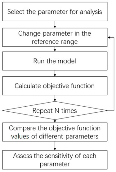
Figure 1.
Procedure of the multi-parameter sensitivity analysis.
As stated above, the MiCES model has already provided a reference range of each parameter. Therefore, in this study, we randomly take 500 numbers evenly distributed in the reference range derived temperature output for each parameter set, then calculated the objective function by Equation (6). At last, we obtain the objective function value within the parameter range. All parameters’ objective function values are calculated both in the prediction period and in the observation period.
4.2. The Output Change Measurement Method
The output change measurement method [19] is used for sensitivity analysis in parameter perturbation. The procedure of the output change measurement method is quite clear. Consider X as parameter set and y(X) as the output, the change in the output induced by a Δ change in parameter can be defined as:
With the change of one parameter, a set of outputs can be obtained, and the statistics of these outputs can be used to characterize the sensitivity of the parameter. We use the mean μ of as index for parameters’ sensitivity, which is dimensionless. Referring to the MiCES, the ratio of the percentage of temperature change to the percentage of parameter change is used as the output factor of the parameter. Each parameter takes the optimization parameter set as the reference point, evenly takes 500 samples from the ±50% range.
To compare with the output measurement method and to see if the results of parameters’ sensitivity are consistent, another index called the Sobol index [20,21], which is one of the most widely used indices for sensitivity analysis, is also used to MiCES model’s parameters. The model parameters are varied within their reference ranges, and the model run N times with different parameter sets, so we get N outputs of the model. The variance of the model output can measure the change by the uncertainty of the parameters. The Sobol index is the ratio of variances of the output if only one parameter is varied while fixing all other parameters to all parameters varied:
It is noted that the Sobol index is also dimensionless.
We run the model 2000 times to get the output samples for each parameter while other parameters fixed in the optimization parameter set, only sensitive parameters are calculated in this case.
5. Results
5.1. Parameter Sensitivity in the Reference Range
As noted above, the objective function f(T) approximately depicts the temperature change caused by the change of a parameter. To compare the sensitivity of different parameters, Figure 2 shows the maximum objective function value of each parameter. Since future climate change is concerned matter, the f(T) in the prediction period (the red point in Figure 2) is used to clarify the parameters. We define the ones with f(T) larger than 0.4 K as sensitive parameters, which is about 10% of temperature change from pre-industry to the 21st century. Under this standard the climate sensitivity parameter λ, land and ocean temperature-driven carbon feedbacks and , the carbon diffusion coefficient , ocean heat capacity , heat diffusion Do and aerosol radiative forcing f1990 as sensitive parameters. We can see those insensitive parameters are preindustrial CO2 concentration, deep–shallow ocean carbon diffusion coefficient, deep ocean initial carbon stock, and all parameters related to CH4 and N2O. It suggests the separation of shallow and deep ocean components in this model is not particularly useful compared to other more simplified 1-layer energy balance models (such as in [22]).
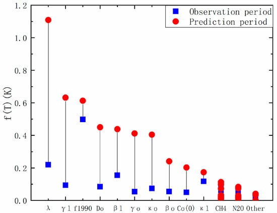
Figure 2.
Maximum objective function values of all parameters in the observation period and prediction period.
Almost all parameters’ f(T) values are larger in the prediction period than those in the observation period, which suggests the length of computing period is an impacting factor to the sensitivities. Some parameters’ f(T) changes less such as f1990 and , which implies they will be less critical in the future.
5.2. Sensitivity of Key Parameters
The parameters related to the heat and carbon transfer are further analyzed using the output change method. As shown in Table 1, the μ value of each parameter changes with time and emission scenarios. Almost all parameters’ μ values decrease in the prediction period with the emission increase, which indicates that the Earth system’s physical process can affect the climate less in the high emission scenario.

Table 1.
Parameters sensitivity of MiCES model (unitless).
The climate sensitivity parameter λ gets the highest μ value in the prediction period and the second high in the observation period. It can be considered as the most sensitive parameter. Compared to the average μ value of each scenario, the f1990′s μ value is about 11% in the prediction period of the observation period, which means the aerosol will be less critical in the future in climate change. This result is in accordance with the multi-parameter sensitivity analysis method.
The results in the control run in which emission stay constant are similar to the scenario runs, the μ value of f1990 is lager, but still less than that during the observation period, which means the process of aerosol becomes less critical whether sulfates’ emissions become less or not.
The computed Sobol indices of key parameters show similar results to the output change method (Table 2).
Table 2.
Sobol index of parameters of MiCES model (in E-03 scale, unitless).
The index value of ocean heat capacity ( will be approximately 50 times larger in the prediction period than in the observation period. It suggests that the ocean as a heat reservoir will become more and more critical in the future climate change, which is consistent with the multi-parameter sensitivity method. The increasing importance of ocean over time is likely to be associated with the rapid and slow heat response of the ocean [23]. Due to the slow warming effect of the deep ocean, the global temperature is no longer synchronized with the radiative forcing. The deep ocean not only delays the rise of global mean temperature when radiative forcing is raised but more importantly, it will play an increasingly important role over time, especially after radiative forcing becomes weak. The temperature-driven carbon feedbacks also become much more sensitive, caused by positive feedback of carbon release of the ecosystem to temperature rise.
Similar to μ value’s result, the Sobol index of f1990 is also less (about 5%) in the prediction period than the observation period, but that of the control run does not decrease that much. It may due to that the emission of sulfate decreases much in all RCP scenarios, while in the control run, aerosol stays at a high level of 2005′s. The result indicates that the temperature uncertainty caused by the aerosol process could be notable if the emission of sulfate does not decrease.
In general, Sobol index is more like an index for uncertainty analysis other than the μ value. It could be the reason why Sobol indices of most parameters increase with the emission increase, which is different from the μ value’s result. This result indicates that the temperature uncertainty caused by parameters, which represent corresponding physical processes, increases with the emission increase.
5.3. Uncertainty Analysis
Since the sensitive parameters can affect the output of the model (the most sensitive one can make a temperature difference more than 0.4 °C or more than 10%), a stricter parameters’ range is needed. To that end, we consider the inputs of the MiCES model as random variables and analyzed the ensembles of simulations with distributions of emission and temperature. According to Gütschow et al. [24], we consider the uncertainty range of emissions as 14%, and the uncertainty range of temperature comes from Frank [25] as ±0.46 °C. Then we run the model multiple times with randomly picked N emissions and N temperatures in their uncertainty range to obtain the parameter uncertainty. As shown in Figure 3, temperature samples produced by getting each time point as a random temperature, while the emission samples are produced by changing the whole series to a random rate. Since only the uncertainty of CO2 emissions is considered, only the parameters directly connected with CO2 are calculated.
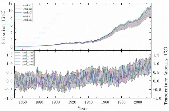
Figure 3.
Random inputs of emission and temperature with grey shaded areas showing the uncertainty range.
As shown in Figure 4, the distributions of key parameters are fitted by several kinds of distributions, to make the residuals smallest: and are fitted by normal distribution; , , and are fitted by extreme value distribution; λ is fitted by burr distribution and is fitted by stable distribution. We define 95% confidence interval as the reference range of each parameter, as shown in Table 3 with Sanderson’s [7] range for comparison. The climate sensitivity parameter’s range is 2.15–5.79 K(Wm−2)−1 at a 95% confidence level, and the expected value is 3.27 K(Wm−2)−1. As shown in Table 3, the expected values of the parameters are significantly different from those suggested by Sanderson’s [7]. Specifically, the range of land and ocean temperature-driven carbon feedbacks and is [−0.5, 0.5] and [0, 0.5] by Sanderson et al. [7]. Due to the reason that more carbon will be released to atmosphere with temperature rise, the parameters are set to be negative as [−200, 0] and are obtained the probability distribution between [−74.0, −45.5] and [−5.92, −0.26] as shown in Figure 4, which are more close to that of Arora [26].
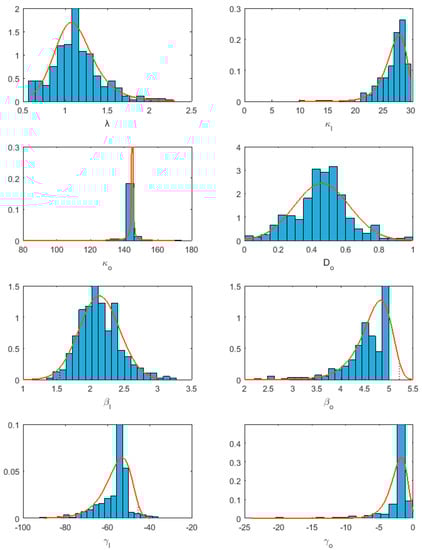
Figure 4.
Parameter distributions by random input of emission and temperature.
Table 3.
Parameters’ uncertainty by random emission and temperature input.
5.4. Application of MiCES Model with Optimal Parameter Sets and Parameters Range
Figure 5 shows the goodness of fitting the observed temperature and emission and the uncertainty range using parameters suggested in Table 3. The uncertainty ranges of estimated temperature and CO2 concentrations are also plotted in the figure with comparison to those of Sanderson’s. The Sanderson’s range of temperature in 2016 is 0.4–3.5 °C, while our calculated temperature is narrowed to 0.6–1.9 °C. For the concentration of CO2 in the atmosphere, our result is 380–470 ppm other than Sanderson’s 375–540 ppm. It can be seen that the observed temperature basically falls within the uncertainty range calculated by our result, and so does the CO2 concentration. The covariance between output temperature and the observed temperature is R2 = 0.903, which implies the high reliability of the expected value of parameters.
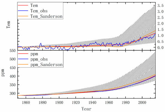
Figure 5.
Model output temperature and CO2 concentration with grey shaded areas showing the uncertainty range and dashed areas show the uncertainty range of Sanderson’s.
We also calculate the impact of the sensitive parameters on model output for comparison. As shown in Figure 6, The most sensitive parameter λ, shows an impact of 0.68 °C, the parameter , which is less sensitive, shows an impact of 0.26 °C. The result shows the importance of sensitive parameters, and the sensitivity analyze gives us a measurement of this importance.
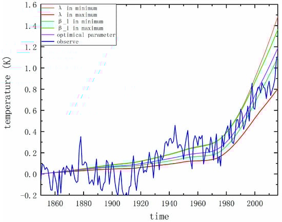
Figure 6.
Sensitive parameters’ impact on model temperature output.
Furthermore, the MiCES model is run to calculate the contribution of each greenhouse gas to temperature increase by running each greenhouse gas only at one time with our optimal parameter set. As shown in Figure 7, fossil fuel’s emission of CO2 is the most critical contributor in GHGs, which caused about 0.84 °C temperature rise from 1850 to 2016. Emissions of CO2 emitted by land-use change, methane, N2O, and other minor GHGs lead to a temperature rise of 0.33 °C, 0.35 °C, 0.12 °C, and 0.25 °C, respectively. Unlike above greenhouse gases, the aerosol has a negative effect on temperature rise, which contributed −0.61 °C in total. As shown in Figure 6, the effect of aerosol, the slope of the curve, is smaller since the 1990s. That is a result of decreasing the emission of sulfate, while on the other hand, the decreasing sensitivity of f1990 (aerosol radiative forcing in 1990) also leads to a less critical aerosol process in the future.
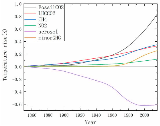
Figure 7.
Different GHGs contributions to temperature rise.
6. Conclusions
In this study, the sensitivity of the parameters of the MiCES model at different time periods is tested by the multi-parameter sensitivity method and the output change measurement method, and the sensitive parameters, as well as the parameters with large variation of sensitivity at different time periods, are discussed. The main conclusions are as follows.
- (1)
- Parameters connected to heat and carbon transfer are sensitive parameters in the MiCES model, while parameters connected to the non-CO2 GHGs are less sensitive. Climate sensitivity parameter, biosphere CO2 fertilization parameter, biosphere temperature response and atmosphere–ocean diffusion coefficient are the most sensitive parameters, which can strongly influence the result of the model.
- (2)
- The sensitivity of ocean heat capacity increases with time and temperature rise, which means the role of the ocean in future climate change is becoming more important. It is possibly due to the slow response of deep oceans to warming, whose contribution to temperature change is growing.
- (3)
- By changing the input as random variables, we obtained the distribution of optimal parameters, and defined the 95% confidence intervals as the reference ranges, which is smaller than the MiCES’s reference range. The climate sensitivity parameter’s range is 2.15–5.79 K(Wm−2)−1 at 95% confidence. And the uncertainty range calculated by the reference ranges is about 1.3 °C in 2016.
- (4)
- Using the optimal set of parameters, MiCES can provide one GHG effect to temperature rise alone, the CO2 emitted by fossil fuel is the most important factor and brings about 0.8 °C temperature rise since 1850 to 2016. Aerosol has a negative effect on the temperature rise by 0.6 °C, which might show less importance in the future.
Through the sensitivity of model parameters and their changes, we can have a certain understanding of the importance of geophysical processes in the climate system and its change with the different conditions. It helps us to quantify the output change affected by parameter perturbation and shows the essential parameters we should pay attention to. This study focused on the parameters of ocean heat capacity and aerosol forcing, the remaining parameters with large variations need further study to understand the geophysical processes from emission to temperature rise. Since the sensitivity calculated in this study is through temperature change, the contribution by time spans and temperature cannot be separated, which should be further analyzed in the future.
Author Contributions
Conceptualization, H.C. and Q.G.; methodology, J.C. and Y.X.; acquisition of data, J.C., H.C. and Y.X.; analysis of measurements, J.C.; writing—original draft, J.C. and H.C.; writing—review and editing, J.C., H.C. and Y.X. All authors have read and agreed to the published version of the manuscript.
Funding
This work was supported by the National Key Research and Development Program of China (Grant Number: 2017YFA0605303), the National Natural Science Foundation of China (41877454), the Strategic Priority Research Program of the Chinese Academy of Sciences (No. XDA23100401), and the Youth Innovation Promotion Association of CAS (No. 2019053).
Conflicts of Interest
The authors declare no conflict of interest.
Appendix A
Table A1.
Parameter ranges for the MiCES model used in this study.
Table A1.
Parameter ranges for the MiCES model used in this study.
| Sub Model | Description | Name | Reference Range |
|---|---|---|---|
| Climate | Climate sensitivity Wm−2 K−1 | λ | [0.6, 3.8] |
| Climate | Land surface heat capacity (Ka−1)−1 Wm−2 | [1, 30] | |
| Climate | Ocean heat capacity (Ka−1)−1 Wm−2 | [1, 300] | |
| Climate | Atmosphere–ocean diffusion coefficient Wm−2 K−1 | Do | [0.001, 1] |
| Climate | Preindustrial CO2 concentration ppm | ppm_1850 | [270, 290] |
| Climate | Biosphere CO2 fertilization parameter Pg ppm−1 | [0, 3] | |
| Climate | Biosphere temperature response Pg K−1 | [−0.5, 0.5] | |
| Climate | Shallow ocean initial carbon stock Pg | Co(0) | [100, 600] |
| Climate | Ocean carbon diffusion parameter Pg ppm−1 | [0, 5] | |
| Climate | Ocean carbon solubility response Pg K−1 | [0, 0.5] | |
| Climate | Deep–shallow ocean carbon diffusion coefficient Pg ppm−1 | [0, 4] | |
| Climate | Deep ocean initial carbon stock Pg | Cod(0) | [20,000, 100,000] |
| Climate | Aerosol 1990 forcing Wm−2 | f1990 | [−3, 0] |
| CH4 | Present-day OH feedback | sOH | [−0.37, −0.27] |
| CH4 | Present-day loss frequency due to tropospheric Cl a−1 | kCl | [0.0025, 0.0075] |
| CH4 | Present-day loss frequency due to all stratospheric processes a−1 | kStrat | [0.0073, 0.02] |
| CH4 | Present-day loss frequency due to surface deposition a−1 | kSurf | [0.004, 0.08] |
| CH4 | Preindustrial concentration ppb | cPI | [650, 750] |
| CH4 | Present-day concentration ppb | cPD | [1600, 1815] |
| CH4 | Present-day growth rate ppb a−1 | dcdt | [4, 6] |
| CH4 | Ratio of PI/PD natural emissions | anPI | [0.8, 1.2] |
| CH4 | Ratio of PI = PD loss frequency due to tropospheric OH | aPI | [0.75, 3] |
| CH4 | Ratio of y2100/PD loss frequency due to tropospheric OH | a2100 | [0.5, 2] |
| CH4 | Present-day methyl-chloroform decay frequency a−1 | kMCF | [0.176, 0.3] |
| CH4 | Present-day MCF loss frequency due to ocean uptake a−1 | kMCFocean | [−0.0071, 0.0071] |
| CH4 | k(Species C OH) = k(MCF C OH) at 272 K | r272 | [0.1, 0.66] |
| N2O | Present-day concentration ppb | cPD | [300, 326] |
| N2O | Present-day growth rate ppb a−1 | dcdt | [0.6, 0.9] |
| N2O | Preindustrial concentration ppb | cPI | [100, 300] |
| N2O | Present-day loss frequency due to all stratospheric processes a−1 | kStrat | [0.007, 0.009] |
| N2O | Ratio of PI/PD loss frequency due to stratosphere, | aPIstrat | [0.75, 1] |
| N2O | Present-day stratosphere feedback(dln(kStrat)/dln(C)) | sStrat | [0.06, 0.2] |
| N2O | Conversion between tropospheric abundance and total burden Tg ppb−1 | b | [4.78, 4.9] |
| N2O | MCF fill factor, global/troposphere mean mixing ratios | fill | [0.96, 1] |
| N2O | Ratio of y2100/PD loss frequency due to stratosphere | a2100strat | [0.9, 1.1] |
| N2O | Ratio of y2100/PD loss frequency due to tropospheric OH | a2100 | [0.9, 1.1] |
| N2O | Ratio of PI/PD loss frequency due to tropospheric OH | aPI | [0.5, 3] |
The differences in Equation (2) between this study and Sanderson’s that’s the original Equation (2) will cause loss of carbon as shown in Figure A1.

Figure A1.
Carbon cycle in the model in our study and original model.
Figure A1.
Carbon cycle in the model in our study and original model.

References
- IPCC. Climate Change 2013: The Physical Science Basis. In Contribution of Working Group I to the Fifth Assessment Report of the Intergovernmental Panel on Climate Change; Stocker, T.F., Qin, D., Plattner, G.-K., Tignor, M., Allen, S.K., Boschung, J., Nauels, A., Xia, Y., Bex, V., Midgley, P.M., et al., Eds.; Cambridge University Press: Cambridge, UK, 2013; p. 1535. [Google Scholar] [CrossRef]
- Keller, D.P.; Lenton, A.; Scott, V.; Vaughan, N.E.; Bauer, N.J.D.; Jones, C.D.; Kravitz, B.; Muri, H.; Zickfeld, K. The Carbon Dioxide Removal Model Intercomparison Project (CDRMIP): Rationale and experimental protocol for CMIP6. Geosci. Model Dev. 2018, 11, 1133–1160. [Google Scholar] [CrossRef]
- Quéré, C.L.; Andrew, R.M.; Friedlingstein, P.; Sitch, S.; Hauck, J.; Pongratz, J.; Pickers, P.A.; Korsbakken, J.I.; Peters, G.P.; Canadell, J.G.; et al. Global Carbon Budget 2018. Earth Syst. Sci. Data 2018, 10, 2141–2194. [Google Scholar] [CrossRef]
- Tung, K.K.; Zhou, J. Using data to attribute episodes of warming and cooling in instrumental records. Proc. Natl. Acad. Sci. USA 2013, 110, 2058–2063. [Google Scholar] [CrossRef] [PubMed]
- Covey, C.; Dai, A.; Lindzen, R.S.; Marsh, D.R. Atmospheric Tides in the Latest Generation of Climate Models. J. Atmos. Sci. 2014, 71, 1905–1913. [Google Scholar] [CrossRef]
- Hu, G.; Zhao, Z. Are Climate Models of IPCC AR5 Getting Better than Before? Clim. Chang. Res. 2014, 10, 45–50. [Google Scholar]
- Sanderson, B.M.; Xu, Y.; Tebaldi, C.; Wehner, M.; O’Neill, B.; Jahn, A.; Pendergrass, A.G.; Lehner, F.; Strand, W.G.; Lin, L.; et al. Community climate simulations to assess avoided impacts in 1.5 and 2 °C futures. Earth Syst. Dyn. 2017, 8, 827–847. [Google Scholar] [CrossRef]
- Culina, J.; Kravtsov, S.; Monahan, A.H. Stochastic Parameterization Schemes for Use in Realistic Climate Models. J. Atmos. Sci. 2011, 68, 284–299. [Google Scholar] [CrossRef]
- Ge, Q.; Wang, S.; Fang, X. An uncertainty analysis of understanding on climate change. Geogr. Res. 2010, 29, 191–203. [Google Scholar]
- James, E.O.; Spillane, M.C.; Percival, D.B.; Wang, M.; Mofjeld, H.O. 2004: Seasonal and regional variation of pan-arctic surface air temperature over the instrumental record. J. Clim. 2004, 17, 3263–3282. [Google Scholar]
- Mauritsen, T.; Stevens, B.; Roeckner, E.; Crueger, T.; Esch, M.; Giorgetta, M.; Haak, H.; Jungclaus, J.; Klocke, D.; Matei, D.; et al. The RCP greenhouse gas concentrations and their extensions from 1765 to 2300. Clim. Chang. 2011, 109, 213–241. [Google Scholar]
- Morrison, H.; Milbrandt, J.A. Parameterization of cloud microphysics based on the prediction of bulk ice particle properties. Part I: Scheme description and idealized tests. J. Atmos. Sci. 2015, 72, 287–311. [Google Scholar] [CrossRef]
- Fletcher, C.G.; Kravitz, B.; Badawy, B. Quantifying uncertainty from aerosol and atmospheric parameters and their impact on climate sensitivity. Atmos. Chem. Phys. 2018, 18, 17529–17543. [Google Scholar] [CrossRef]
- Morales, A.; Posselt, D.J.; Morrison, H.; He, F. Assessing the Influence of Microphysical and Environmental Parameter Perturbations on Orographic Precipitation. J. Atmos. Sci. 2019, 76, 1373–1395. [Google Scholar] [CrossRef]
- Covey, C.; Lucas, D.D.; Tannahill, J.; Garaizar, X.; Klein, R. Efficient screening of climate model sensitivity to a large number of perturbed input parameters. J. Adv. Model. Earth Syst. 2013, 5, 598–610. [Google Scholar] [CrossRef]
- Choi, J.; Harvey, J.; Conklin, M.H. Use of multi-parameter sensitivity analysis to determine relative importance of factors influencing natural attenuation of mining contaminants. In Proceedings of the Toxic Substances Hydrology Program Meeting, Charleston, SC, USA, 8–12 March 1999. [Google Scholar]
- Prather, M.J.; Holmes, C.D.; Hsu, J. Reactive greenhouse gas scenarios: Systematic exploration of uncertainties and the role of atmospheric chemistry. Geophys. Res. Lett. 2012, 39, L09803. [Google Scholar] [CrossRef]
- Myhre, G.; Highwood, E.J.; Shine, K.P.; Stordal, F. New estimates of radiative forcing due to well mixed greenhouse gases. Geophys. Res. Lett. 1998, 25, 2715–2718. [Google Scholar] [CrossRef]
- Morris, M.D. Factorial sampling plans for preliminary computational experiments. Technometrics 1991, 33, 161–174. [Google Scholar] [CrossRef]
- Sobol’, I.M. Sensitivity analysis for non-linear mathematical models. Math. Modeling Comput. Exp. 1993, 1, 407–414. [Google Scholar]
- Mai, J.; Tolson, B.A. Model Variable Augmentation (MVA) for Diagnostic Assessment of Sensitivity Analysis Results. Water Resour. Res. 2019, 55, 2631–2651. [Google Scholar] [CrossRef]
- Xu, Y.; Ramanathan, V. Well below 2 °C: Mitigation strategies for avoiding dangerous to catastrophic climate changes. Proc. Natl. Acad. Sci. USA 2017, 114, 10315–10323. [Google Scholar] [CrossRef]
- Long, S.M.; Xie, S.P.; Liu, Q.; Zheng, X.T.; Huang, G.; Hu, K.; Du, Y. Slow ocean response and the 1.5 and 2 °C warming targets. Chin. Sci. Bull. 2018, 63, 558–570. [Google Scholar] [CrossRef]
- Gütschow, J.; Jeffery, M.L.; Gieseke, R.; Gebel, R.; Stevens, D.; Krapp, M.; da Rocha, M.F. The PRIMAP-hist national historical emissions time series. Earth Syst. Sci. Data 2016, 8, 571–603. [Google Scholar] [CrossRef]
- Frank, P. Uncertainty in the Global Average Surface Air Temperature Index: A Representative Lower Limit. Energy Environ. 2010, 21, 969–989. [Google Scholar] [CrossRef]
- Arora, V.K.; Boer, G.J.; Friedlingstein, P.; Eby, M.; Jones, C.D.; Christian, J.R.; Bonan, G.; Bopp, L.; Brovkin, V.; Cadule, P.; et al. Carbon-concentration and carbon-climate feedbacks in CMIP5 Earth System Models. J. Clim. 2013, 26, 5289–5314. [Google Scholar] [CrossRef]


© 2020 by the authors. Licensee MDPI, Basel, Switzerland. This article is an open access article distributed under the terms and conditions of the Creative Commons Attribution (CC BY) license (http://creativecommons.org/licenses/by/4.0/).