Abstract
The high-frequency monitoring of three-dimensional wind fields is crucial in planetary boundary layer meteorology. Doppler wind lidar and meteorological towers are the most important instruments for site observations of three-dimensional wind fields. This study systematically investigated and compared the performances of three wind measurement instruments: A Doppler wind lidar (Windcube 100s), cup anemometer/wind vane and sonic wind anemometer mounted on the 325 m meteorological tower in the polluted urban city of Beijing. The horizontal wind speed measurements of the Doppler wind lidar closely matched those of the cup anemometer and the sonic wind anemometer with high coefficients of determination (R2: 0.79–0.96 and 0.90–0.97, respectively). Moreover, the results also showed good agreement between the three measurements of the prevailing horizontal wind direction. Conversely, there were weak correlations between the vertical wind speeds of the Doppler wind lidar and sonic wind anemometer with low coefficients of determination (R2: 0.30–0.46). With increasing temporal scale, the consistency in the vertical wind increased. In addition, the Doppler wind lidar seemed to correlate better with the sonic wind anemometer at heights exceeding 300 m (R2: 0.48–0.77). Note that there was a remarkable difference between the Doppler wind lidar and 325 m meteorological tower observations as the aerosol concentrations changed rapidly. Different wind measurement instruments have unique advantages and are thus irreplaceable. The Doppler wind lidar is better at measuring larger turbulent eddies.
1. Introduction
As a fundamental physical element of the planetary boundary layer, wind has profound impacts on the environment, climate, energy and weather phenomena [1,2,3,4]. Currently, there are many ways to measure and monitor wind. The traditional and most common measurement is to acquire observations from a meteorological tower, but the height of this measurement is greatly limited [5,6,7]. Radiosondes can obtain wind fields at high altitudes, but it is impossible to make continuous observations with a high frequency. Meanwhile, radiosondes cannot measure vertical wind [8]. Sodar is able to use sound echoes to detect wind profiles; however, this technique is a short-term profiler. It is unable to measure high wind speed (>15 m s−1). In recent years, Doppler wind lidar (DWL) has gradually become a promising remote sensing instrument for wind observations by remedying the disadvantages of other instruments [9,10]. Therefore, it is of great practical significance to validate the DWL measurement before it can be widely acknowledged.
Validation analyses of DWL data have been conducted by many scholars. Near the surface, DWL data were compared with meteorological tower data at the Department of Energy’s National Renewable Energy Laboratory (NREL), Golden, CO, USA. It was found that the horizontal wind speeds measured by these two observation measurements are highly consistent [6]. Similarly, new measurement techniques were tested in the eXperimental Planetary boundary layer Instrumentation Assessment (XPIA), and the same conclusion was obtained [11]. Some scholars used radiosondes to validate DWL data at high altitudes in Norway and Germany, and the new remote sensing technique showed better wind measuring performances [12,13]. In this context, studies have been conducted not only on land but also over the sea. The correlation coefficient between DWL and meteorological tower data was 0.99 on an offshore platform (FINO1) [5]. In addition, mobile airborne and ship-borne DWL sensors are considered ideal instruments for the Atlantic and Arctic [14,15]. In conclusion, all these studies have confirmed that DWL is a good choice for observing wind.
The above studies provided a certain understanding of DWL, but there are still some problems to be solved. The majority of validations were concentrated in Europe and the United States, which exhibit relatively clean air and low concentrations of particulate matter with a diameter of less than 2.5 μm (PM2.5: 6–13 μg m−3) [5,6,12,15]. In rapidly developing China, severe urban pollution is a significant concern with high concentrations of aerosols [16,17,18,19]. This has led most researchers to explore local pollution mechanisms and solutions. There is no doubt that meteorological factors (wind, temperature and relative humidity) have a great influence on the pollution. The impacts of the wind are mainly reflected in the process of pollution transmission and elimination. Therefore, high-frequency and real-time DWL is urgently needed to observe the local wind fields. The measurement of DWL is closely related to the local aerosols. The particulate matter concentrations rapidly decrease as pollution weakens quickly in a short time. During this period, the performance of DWL is still unknown. In view of this uncertainty, three-dimensional DWL data are validated by observations from the 325 m meteorological tower in the polluted city of Beijing, the findings of which will provide a reference for future research.
2. Experiment and Methodology
2.1. Observation Site and Instruments
The observation site is a typical urban station and is located at the State Key Laboratory of Atmospheric Boundary Layer Physics and Atmospheric Chemistry (LAPC) (39°58′ N, 116°22′ E, altitude: 49 m) in urban Beijing. The LAPC is mainly covered by residential houses, city parks with heights of 15–20 m and tall offices buildings with heights of 70–90 m. More details about the surroundings of the LAPC can be found in Al-Jiboori and Hu’s literature [20]. With the rapid development of the city, the local pollution problem has been gradually exposed [21].
Figure 1 and Table 1 show the observation field, instruments and related parameters. The 325 m meteorological tower is the highest in North China and has provided a great number of details regarding the PBL in the urban area [22,23,24]. The tower has a total of 15 observation platforms of 8, 15, 32, 47, 63, 80, 102, 120, 140, 160, 180, 200, 240, 280 and 320 m at aboveground levels (AGLs). Each platform is equipped with two cup anemometers (MetOne 010c, MetOne, USA) and a wind vane (MetOne 020c, MetOne, Grants Pass, OR, USA) with a temporal resolution of 0.05 Hz. Moreover, a sonic wind anemometer (Windmaster, Gill Instruments, Lymington, Hampshire, UK) is installed on the platforms at 47, 140 and 280 m AGLs with a temporal resolution of 10 Hz. The 325 m meteorological tower support is in the southeast–northwest direction, which is consistent with the prevailing local wind direction. The metal tower has a 2.7 m face width and an open construction with triangular shape to reduce wake effects near the instruments; thus, the measured data are of high quality according to the recommended criteria [20,25]. The cup anemometer has a starting wind speed (0.22 m s−1) and a maximum wind speed (60 m s−1). Therefore, this study uses the data of the wind anemometer with a wind speed of 0.22–60 m s−1 for verification and validation. In addition, we only choose the wind data as a reference when the two cup anemometers measure the same horizontal wind speed. Vertical and horizontal wind profiles are retrieved by DWL (Windcube 100s, Leosphere, Saclay, France). The particulate matter 2.5 (PM2.5) analyser is located at 8 m AGL in Beijing (RP 1400, Thermo, Waltham, MA, USA).
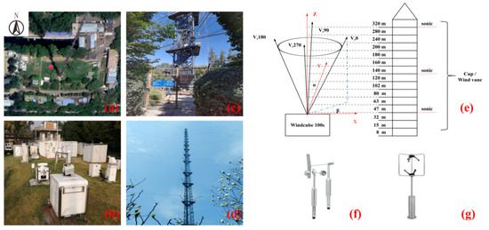
Figure 1.
Photos of the observation field and instruments. The left panels show the (a) 325 m meteorological tower and (b) Doppler wind lidar (DWL) (Windcube 100s) in the yard. The (c) close-up and (d) prospect view of the 325 m meteorological tower in the middle panels. The top-right picture presents (e) the measurement principle of the DWL and the aboveground levels (AGLs) of the meteorological tower. The bottom-right pictures display the observation instruments: (f) Cup anemometer and wind vane (MetOne 010C and MetOne 020C), (g) the sonic wind anemometer (Windmaster). The red dot in (a) is the position of the Windcube 100s.

Table 1.
The detection resolution, accuracy, range and level of the instruments in the experiment.
The wind sensors of the cup anemometer and wind vane are, more specifically, a durable three-cup anemometer and a lightweight airfoil vane, respectively, which have the same measurement principle. The three-cup anemometer and lightweight airfoil vane both rotate around a vertical shaft driven by wind power. The horizontal wind is directly proportional to the rotation around this shaft [26,27].
The measurement principle of the sonic wind anemometer is the sonic time-difference method. The core of the time-difference method is the superposition of ultrasonic waves on the airflow path. If the propagation direction of the sonic wave is the same as the air flow path, the speed of the sonic wave will increase; conversely, if the direction of the sonic wave is opposite to the airflow path, the speed of the sonic wave will decrease. Therefore, the sonic wave speed corresponds to the wind direction under fixed detection conditions. Accurate wind speed and wind direction observations can be obtained as a function of the sonic wave speed and airflow path.
By contrast, the principle of DWL is the Doppler effect, which has a strong relationship with aerosol particles (dust, water droplets, polluted aerosols, salt crystals, biomass burning aerosols in clouds and fog, etc.). DWL emits a fixed pulse signal into the atmosphere. When these electromagnetic waves encounter moving particles, the frequency of the pulse signal changes. By analysing the frequency shift of the backscattered signal, the DWL precisely retrieves the radial wind speed and direction.
During the observation period from 1 to 9 December 2018, the DWL was positioned 20 m to the northwest of the 325 m meteorological tower. The Windcube 100s is designed to include a total of four scanning modes for different applications: Range height indicator (RHI) scan mode, plan position indicator (PPI) scan mode, line-of-sight (LOS) scan mode, Doppler beam swinging (DBS) scan mode [11]. In this study, we used the DBS mode to obtain horizontal and vertical wind for validation. In DBS mode, the lidar scanning head points a beam along 5 different lines of sight, including 4 lines spaced 90° apart at a fixed half-opening angle (0° is vertical) of 15° and 1 vertical line, to obtain the wind field distribution at each different height.
Each DBS mode cycle time is about 20 s (including 4 lines and 1 vertical), so the time resolutions of the horizontal and vertical wind of the DWL are 0.2 and 0.05 Hz. Although the range gates of the DWL are 25, 50, 75 or 100 m (25 m is used in this study), the DWL can output data of 63 and 80 m AGLs and other heights corresponding to the anemometer measurement heights by the sliding average method.
2.2. Retrieval Methods and Data Processing
The wind speed measured by DWL is the radial wind speed. The half-opening angle and azimuth of the laser beam emitted by the Windcube 100s are α (15°) and β, respectively (Figure 1c). The radial wind speed is Vr, and the radial wind speeds in the four azimuths, namely, north, east, south and west, are Vr0, Vr90, Vr180 and Vr270, respectively. According to the above variables, the wind speed V can be obtained by using a trigonometric relationship (Vu and Vv represent the horizontal components, while Vw represents the vertical component). The calculation equation is as follows [5]:
These laser beams by the DWL form cone scans composed of different circles. Therefore, the DWL conversion method relies on the premise that the horizontal wind speed within a circle is uniform, which is also called the homogeneity assumption.
As the smallest detection range of the Windcube 100s is 50 m, this study used observation data from 47, 63, 80, 102, 120, 140, 160, 200, 240, 280 and 320 m AGLs of the meteorological tower for the validation analysis. There was no precipitation during the observation period. Considering the signal-to-noise ratio (SNR) threshold, values with SNR < −26 dB were discarded from the DWL data. The data are averaged each minute or hour for comparison purposes. Due to the problem of the false transformation of the wind direction at 0°, the wind speed and direction are uniform based on the method of vector averaging [28,29], as defined in Equation (2); at the same time, the DWL data are converted according to Equation (3).
In Equation (2), Vi, Xi, Yi and γi represent the measured horizontal wind speed, the components along the X and Y axes, and the horizontal wind direction at the ith time, respectively. The number of samples during the average time period is N. V, X, Y and γ are the average horizontal wind speed, the components along the X and Y axes, and the average horizontal wind direction, respectively.
In Equation (3), θ1 is the horizontal wind direction measured by the wind vane on the 325 m meteorological tower, and θ2 and θ3 are the horizontal wind directions of the Windcube 100s before and after conversion, respectively.
To discuss the differences between three measurements, we used the values of wind speeds or wind directions by the DWL minus cup anemometer/wind van or sonic wind anemometer in Equation (4). The differences in horizontal wind speeds and directions by the DWL and wind vane are SDC and DDC, respectively. The differences in horizontal wind speeds and directions by the DWL and sonic wind anemometer are SDS and DDS, respectively, while the difference in vertical wind speeds by the DWL and sonic wind anemometer is VDS. The values of horizontal wind speeds of the DWL, cup and sonic wind anemometer are HSD, HSC and HSS, respectively. The values of horizontal wind directions of the DWL, cup and sonic wind anemometer are HDD, HDC and HDS, respectively. The values of vertical wind speeds of the DWL and sonic wind anemometer are VSD and VSS, respectively.
In Equation (5), the turbulent kinetic energy (TKE) is calculated, and the two horizontal wind standard deviations and the vertical wind standard deviation are δu, δv and δw, respectively. In order to improve the quality of TKE by the DWL and sonic wind anemometer, we have made corrections applied to account for coordinate rotation, variance contamination, etc. [30,31].
3. The General Situation during Pollution Episodes over Beijing
Pollution in Beijing has long been a challenging problem during autumn and winter [32,33]. To solve this problem, researchers need to understand the physical and chemical processes of pollution in detail. The meteorological factors (wind, temperature, relative humidity, etc.) have a great impact on pollution. DWL is an attractive alternative for obtaining the local continuous three-dimensional wind field. However, the most validations of DWL have basically been focused on clear environments. The application of DWL in contaminated areas remains unclear. Hence, it is essential and appropriate to test the DWL performance under different pollution conditions.
The hourly temporal variations in PM2.5 along the horizontal and vertical wind profiles obtained by DWL during 1–9 December 2018 are shown in Figure 2a,b. In general, the average horizontal and vertical wind speeds were 7.8 and 0.2 m s−1, respectively, and the prevailing wind was dominated by a strong northerly or weak southerly wind during the observation period. Notably, typical pollution occurred during 1–3 December. From 1 December to the night of 2 December, the southerly wind was dominant, and the local average horizontal and vertical wind speeds were 3.7 and 0.02 m s−1, respectively. Compared to that in the other time periods, the PM2.5 concentration rapidly increased from 59 to 174 μg m−3 in response to the weak southerly wind. Over time, the northerly wind invaded the region from the early morning to the evening of 3 December. The northerly wind was the prevailing wind, and the average horizontal and vertical wind speeds were 13.5 and 0.3 m s−1, respectively. Evidently, PM2.5 dropped rapidly under the strong north wind with an average PM2.5 of 23 μg m−3. It also reflected that the southerly wind would carry pollutants towards the site, whereas the northerly wind would bring in cleaner air [21]. In Figure 2, there was an anti-correlation between wind speed and PM2.5 concentration, suggesting that a calm condition is favourable for air pollution accumulation or haze events. From 3 to 9 December, pollution was negligible and the environment was relatively clean compared to the period of 1–3 December. Northerly and southerly winds dominated the area alternately with average horizontal and vertical wind speeds of 7.6 and 0.2 m s−1, respectively.
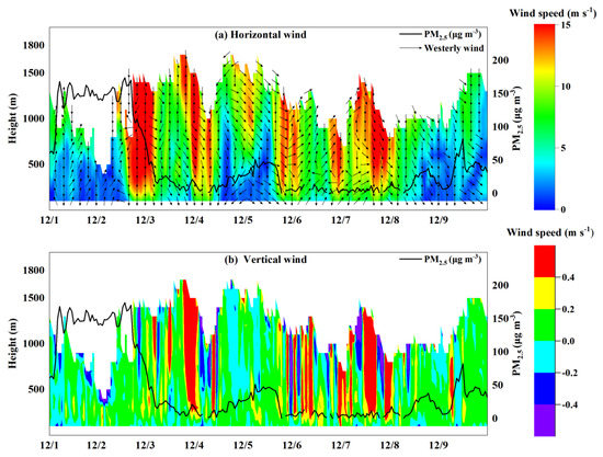
Figure 2.
Temporal hourly variations in the (a) horizontal and (b) vertical wind profiles measured by the DWL. The black line is the temporal hourly variation in PM2.5. The arrows represent horizontal wind directions. The positive and negative values in (b) represent vertical upward and downward wind speeds, respectively.
4. Horizontal Wind Validation of the DWL by a Cup Anemometer and Wind Vane
The cup anemometer and wind vane are considered robust and accurate instruments for measuring horizontal wind. To better understand the applicability and optimization of the DWL in a polluted urban area, we used data from a cup anemometer and wind vane to systematically validate the DWL observations. Figure 3a,b depict the hourly horizontal wind profiles of the DWL and the cup anemometer/wind vane. The variations in the horizontal wind speed and direction measured by the two instruments were generally consistent. It is clear from the DWL and the cup anemometer/wind vane that pollutants accumulated under the weak south wind and dissipated under the strong north wind. In addition, the measurements also reflected the same temporal and spatial changes under clear-sky conditions.
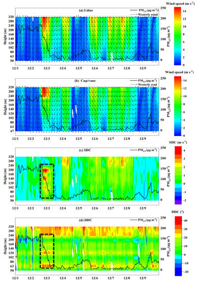
Figure 3.
Temporal hourly horizontal wind variations in the (a) DWL and (b) cup anemometer/wind vane, and in the (c) horizontal wind speed difference SDC and (d) horizontal wind direction difference DDC between the DWL and cup anemometer/wind vane below 325 m. The black line is the temporal hourly variation in PM2.5. The arrows represent horizontal wind directions. The black dashed boxes denote the period of rapid change of aerosol loadings.
As shown in Figure 3c, there was an hourly average difference in SDC of 0.6 m s−1 in the wind speed between the DWL and cup anemometer. It was apparent that the difference in speed reached the maximum of 1.7 m s−1 under strong winds, when the aerosols changed dramatically as the pollution decreased rapidly. Under clear-sky conditions, the horizontal difference in speed was prominent under strong winds. As the height increased, the difference continued to increase. Compared to that under clear-sky conditions, this difference in speed was reflected along the whole height when PM2.5 varied widely. This phenomenon has rarely been reported in previous studies.
The difference in wind direction was not the same as the hourly difference in wind speed (Figure 3d). The difference in the wind direction of DDC exhibited a varying distribution with height. In addition, a notable difference in the wind direction (26°) was also evident with a drastic increase in PM2.5. The surrounding environment also plays an important role in the wind direction. The observation site is a typical urban station. The buildings around the LAPC greatly influence the measurements from the 325 m meteorological tower at different heights [20]. The laser beams emitted by the DWL have a constant half-opening angle of 15°, thereby reducing the influences of surrounding houses and buildings. This may cause large differences in the wind directions at specific altitudes.
Figure 4a shows the temporal hourly variations in the PM2.5 and SNR at 102 m AGL. The temporal variations in the PM2.5 and SNR were almost the same, especially during the pollution process. SNR can be seen as the response of the DWL to the concentration of aerosols in the atmosphere. SNR also weakened rapidly with the aerosols decreasing quickly, indicating that the DWL had a close response to the dissipation of the pollution. Figure 4b shows scatter plots of the minute horizontal wind speeds measured by the DWL and cup anemometer in a clear environment and when pollution is rapidly eliminated. The slope, offset, correlation of determination (R2), root-mean-square error (RMSE) and number of match-ups (N) are also shown in the scatter plots. The R2 and slope between the DWL and cup anemometer decreased significantly from 0.90 to 0.66, and 1.06 to 0.78, respectively, while RMSE increased from 1.40 to 2.16 m s−1 when pollution rapidly weakened. The difference between the DWL and cup anemometer was clear indeed when PM2.5 rapidly decreased. The DWL had better performance in wind speed and direction compared to other instruments for the reason of better SNR during the most polluted time. The situation of aerosols changing rapidly may also reflect that the wind is highly unsteady even within a single lidar wind retrieval duration, which is also an assumption for single lidar retrieval of mean wind.
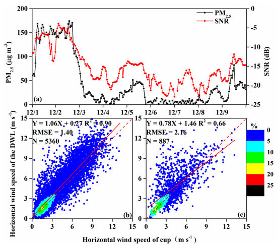
Figure 4.
Temporal hourly variations in the (a) PM2.5 and SNR, and the scatter plots of the minute horizontal wind speeds measured by the DWL and cup anemometer (b) in the clean environment and when (c) pollution is rapidly eliminated from 102 m AGL. The black and red line are the temporal variations in PM2.5 and SNR, respectively. The dashed and solid lines are the 1:1 line and the linear regression, respectively. The text in the upper left describes the linear fitting equation, R2, root-mean-square error (RMSE) and N.
Although atmospheric particulate matter has undergone drastic changes in pollution accumulation and elimination, the wind speed changes in these two processes are obviously different. The overall wind speeds during the accumulation are small and change slowly, which are conducive to the accumulation of particulate matter, while the overall wind speeds during the elimination are high and change quickly, which are conducive to the elimination of pollutants. Aerosol changes at different wind speeds may cause different performances between the DWL and wind cup under accumulation and elimination of pollution. Based on these different measurement principles, different results are obtained with the DWL and cup anemometer. When the concentration of particulate matter decreases rapidly under strong and quickly changing winds, the DWL is likely to be affected according to the Doppler effect, while the cup anemometer and wind vane depend on wind power. However, the decrease in aerosol loading would not significantly affect the average wind speed measurement and would slightly increase the uncertainty in the measurement as the SNR decreases [34].
To systematically validate the accuracy between the DWL and meteorological tower observations, we used the minute horizontal wind data of horizontal wind at the 11 AGLs on the mast for validation. Scatter plots of the cup anemometer and DWL measurements are displayed in Figure 5, which shows good agreement between the DWL and cup anemometer with a high R2 of 0.92. This result is identical to those of most previous studies. In contrast to the wind profiles from the DWL and meteorological tower discussed herein, most researchers are often concerned with comparing scattered data and correlating the measurements between these instruments, whereas little attention is given to the process. Via a statistical analysis of the scatter plots, a close correlation can be observed (Figure 5). However, no difference between the two observations during the pollution dissipation process can be distinguished (Figure 3c,d). It is necessary to combine statistical analysis with process analysis.
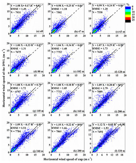
Figure 5.
Scatter plots of the minute horizontal wind speeds measured by the DWL and cup anemometer from (a) all AGLs and (b–l) 50–320 m AGLs. The horizontal data are sorted into multiple cases according to the ordered pairs at an interval of 0.5 m s−1. The colourful dots represent the percentages of the ordered pairs, shown specifically by the colour bar to the right of (c). The dashed and solid lines are the 1:1 line and the linear regression, respectively. The text in the upper left describes the linear fitting equation, R2, RMSE and the N.
As shown in Figure 5b–l, there was no significant difference in the horizontal wind speed between the DWL and cup anemometer within the range of the fitting slope (0.98–1.0) below 100 m AGL. However, the horizontal wind speed measured by the DWL was slightly higher than that measured by the cup anemometer within the range of the fitting slope (1.04–1.12) above 100 m AGL. From 100 to 320 m AGLs, the fitting curve was slightly offset upwards from the 1:1 line. This result indicates that as the horizontal wind speed increased, the difference between the horizontal wind speeds measured by the DWL and cup anemometer increased between 100 and 320 m.
As mentioned earlier, the DWL was in the DBS mode. In fact, there are other methods of the DWL used to obtain horizontal and vertical winds, such as velocity–azimuth-display (VAD) and six-beam method [35]. Most methods are customer-defined and do not rely on the pre-programmed feature of the Windcube software (DBS mode). According to the DBS mode, DWL retrieves the radial speed based on the Doppler effect. Therefore, it is necessary to convert the radial speed measured by the DWL into the wind speed. This conversion principle depends on the premise of the homogeneity assumption. However, as the height increases, the circular surface continues to expand, and the horizontal wind speed in the circular surface is less uniform. At high altitudes, the validity of this assumption fails completely. Consequently, inhomogeneity in the flow may make a difference between DWL and the cup anemometers at greater heights.
So far, the difference in DWL measurement mainly comes from the principle of heterogeneity assumption. Theoretically speaking, the maximum detection distance of Windcube 100s is 3000 m. It requires the wind speed and direction of a circular surface to be consistent in a radius of about 804 m. Such assumptions are difficult to meet at high altitudes. Near the ground, the maximum detection distance of the 325 m meteorological tower is 320 m, so the wind in a circular surface with a radius of 84 m needs to be uniform. From the length of the radius, the heterogeneity assumption at low height performs better than at 3000 m.
The differences caused by the heterogeneity assumption are different under various wind speed conditions. We define the average wind speeds of whole layers less than 5 m s−1 as the smaller wind speed, and wind speeds greater than 5 m s−1 as the larger wind speed. In smaller wind speed scenarios, the average difference in the wind speed at 50 m is 0.16 and 0.33 m s−1 at 320 m. In larger wind speed conditions, it is 0.41 m s−1 at 50 m and 1.56 m s−1 at 320 m. Therefore, it could be concluded that the deviation in larger wind speed is more than that in smaller wind speed.
The RMSE would be expected to increase with the inhomogeneity assumption being violated at higher altitudes. However, it reaches high values at 120, 140 and 200 m AGLs and decreases with altitude afterwards. The surrounding buildings in the city affect not only the measurement of wind direction but also the wind speed, and may be a significant contributing factor to the observed wind speed differences as well. However, this effect on wind speed is not as obvious as the wind direction with the temporal variation. Therefore, different detection principles, urban buildings and aerosol concentrations in the environment have caused different performances in DWL and cup measurements.
Considering the change in the horizontal wind direction at 0°, wind frequency roses (sixteen wind directions) plotted at a 15° angular resolution [36] were used to compare the horizontal wind direction between the DWL and wind vane, as shown in Figure 6a–l. Overall, the DWL observed a peak in the northerly wind direction. By comparison, the horizontal wind distribution of the vane exhibited a peak mainly in the west-northwesterly or northwesterly wind direction. It is apparent that the prevailing wind direction of the DWL was slightly farther towards the north than that of the wind vane. Before the observations, the two measurements had to be aligned due north. However, the geographical North Pole is not a fixed point. In the process of setting the instruments to face north, there is an inevitable introduced error. This may be an important reason for the differences in the wind direction measurements [5,37].
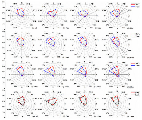
Figure 6.
Wind frequency roses from the (a–l) DWL and wind vane and from the (m–p) DWL and sonic wind anemometer. The vertical axes on the left represent the values of the wind direction frequencies.
At present, there are a lot of validations of the DWL by the meteorological tower. The regional representation of these analyses varies widely, such as mountain, ocean, agricultural fields, airport, coastline and bridge [5,6,7,8,9,10,11,12,13,14,15,34,35,38,39,40,41]. However, validations are relatively few in polluted areas. Some results show that the accuracy of the DWL increases with the SNR [34]. However, when the pollution is rapidly weakened, even if the overall PM2.5 is at a relatively high level, the uncertainty of the DWL also increases. Most of the meteorological towers participating in the above validations are located below 300 m, and the level distributions of these towers are far less than that of the 325 m meteorological tower in Beijing. Many results only show close correlation with the RMSE and gradually increase with height between the DWL and meteorological tower [6,7]. Instead, the wind in urban areas is easily affected by buildings near the ground, and the overall performance between the DWL and meteorological tower does not increase with height.
5. Three-Dimensional Wind Validation of the DWL by a Sonic Wind Anemometer
5.1. Horizontal Wind Validation of the DWL by a Sonic Wind Anemometer
Although the comparison between the DWL and the cup anemometer provides a better understanding of this remote sensing technique, the comparison results are still far from sufficient. Given the attractive features of three-dimensional wind observations by a DWL, a sonic wind anemometer was further used to validate the lidar system. Generally, the hourly variations in the horizontal wind speed and wind direction obtained by the DWL were consistent with those imaged by the sonic wind anemometer (Figure 7a,b). Considering the results shown in Figure 3 and Figure 7, the hourly temporal variations in the horizontal wind measured by the DWL, the cup anemometer/wind vane and the sonic wind anemometer were almost the same. On both hazy and clean days, there was barely any difference among the measurements of the three wind instruments. Figure 7c,d describe the hourly horizontal differences in the wind speed and wind direction of SDS and DDS between the DWL and the sonic wind anemometer. The horizontal wind difference between the DWL and the sonic wind anemometer was not similar to that between the DWL and the cup anemometer/wind vane (Figure 7c,d). Moreover, there was no significant horizontal difference between the DWL and the sonic wind anemometer, as the aerosols changed dramatically.
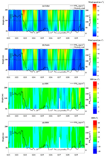
Figure 7.
Temporal hourly horizontal variations in the (a) DWL and (b) sonic wind anemometer, and in the (c) horizontal wind speed difference SDS and (d) horizontal wind direction difference DDS between the DWL and sonic wind anemometer below 325 m. The black line is the temporal hourly variation in PM2.5. The arrows represent horizontal wind directions.
Figure 8a–l show scatter plots of the horizontal wind speed between the DWL and sonic wind anemometer at different time scales at 47, 140 and 280 m AGLs. Values of the R2, slope, offset, N and RMSE are tabulated in Table 2. The horizontal wind speed was mainly concentrated within 0–5 m s−1. This is in accordance with the results of the comparison between the DWL and cup anemometer. In addition, the horizontal wind speeds of the DWL and sonic wind anemometer also demonstrated good agreement with slopes of 0.89–1.07 and R2 values of 0.90–0.99. The prevailing wind directions measured by the DWL and sonic wind anemometer were almost identical (Figure 6m–p). The prevailing wind directions from the sonic wind anemometer were mainly northerly, north-northwesterly and northwesterly at 47, 140 and 280 m AGLs, respectively, which are similar to the prevailing wind directions of the DWL. In conclusion, considering the comprehensive results from the DWL, cup anemometer/wind vane and sonic wind anemometer on the 325 m meteorological tower, DWL is a reliable observation measurement for measuring horizontal wind profiles in the polluted urban area.
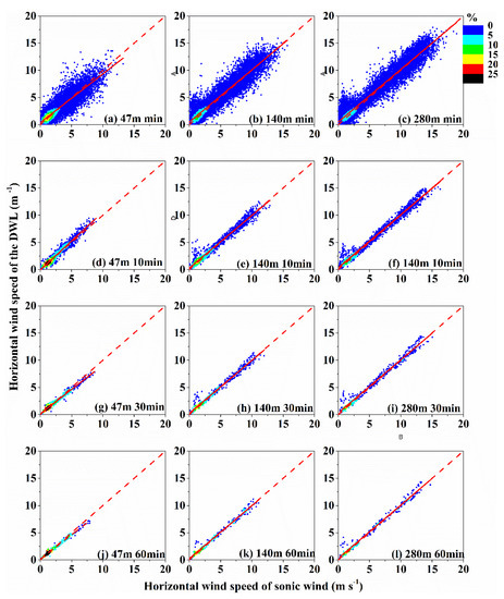
Figure 8.
Scatter plots of the horizontal wind speeds at different temporal scales of (a–c) 1, (d–f) 10, (g–i) 30 and (j–l) 60 min by the DWL and sonic wind anemometer at 47, 140 and 280 m AGLs. The horizontal data are sorted into multiple cases according to the ordered pairs at an interval of 0.5 m s−1. The colourful dots represent the percentages of the ordered pairs in each case, shown specifically by the colour bar to the right of (c). The dashed and solid lines are the 1:1 line and the linear regression, respectively.
Table 2.
The linear regressions, R2, N, RMSE and biases between DWL and sonic wind anemometer.
5.2. Vertical Wind Validation of the DWL by a Sonic Wind Anemometer
The key application of DWL is to retrieve vertical wind observations, which is an advantage over most wind measurement instruments. The sonic wind anemometer also has the excellent ability to measure vertical wind. Therefore, the vertical wind of the DWL was evaluated by a comparison with measurements from the sonic wind anemometer. The hourly temporal variation in the vertical wind profiles by the DWL and sonic wind anemometer are displayed in Figure 9a,b. In contrast to the variations in the horizontal wind, the variation in the vertical wind by the DWL was different from that by the sonic wind anemometer. The variation in the vertical wind profile observed by the DWL was not as obvious as that by the sonic wind anemometer under strong vertical winds, especially when the aerosols changed drastically. Compared to the variations in the horizontal wind (Figure 3a,b and Figure 9a,b), the variations in the vertical wind observed by the sonic wind anemometer seemed more in accordance with the actual changes. The high horizontal wind speeds by the sonic wind anemometer almost corresponded to the high vertical wind speeds. The differences in the vertical wind speeds of VDS between the DWL and sonic wind anemometer are reflected in Figure 9c. The differences in the vertical wind speed were concentrated under strong winds. The vertical difference became increasingly remarkable as the aerosols changed dramatically. It could be due to either the sonic wind anemometers or DWL not being perfectly level, so some of the horizontal wind is projected into the vertical. Furthermore, this effect could affect the DWL and sonic wind anemometer differently, amplifying the observed differences, depending on the attitude (pitch, roll) of the sensors. This could largely explain the differences in Figure 9c.
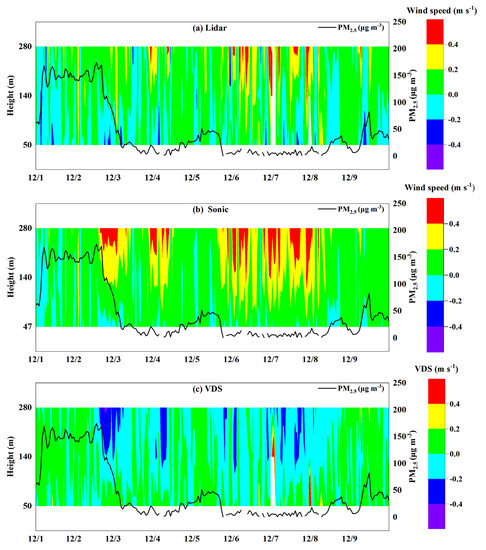
Figure 9.
Temporal hourly vertical variations in the (a) DWL and (b) sonic wind anemometer and in the (c) vertical wind speed difference (VDS) between the DWL and sonic wind anemometer (the value of vertical wind speed by DWL minus sonic wind anemometer) below 325 m. The black line is the temporal hourly variation in PM2.5. The positive and negative values in (a,b) represent upward and downward wind speeds, respectively.
The correlation analysis of the vertical wind speeds (absolute values) at different temporal scales is represented in Figure 10 and Table 2. On the minute time scale, the vertical wind speeds between the DWL and sonic wind anemometer exhibited a low correlation with slopes of 0.41–0.52 and R2 values of 0.3–0.46 at 47, 140 and 280 m AGLs. These findings are also different from the correlation analysis of the horizontal wind speeds. The vertical wind correlation improved with increasing time scale, and the improvement was most obvious at 280 m (from 0.46 to 0.77). The DWL seemed to correlate better with the sonic wind anemometer at high altitudes than at low altitudes. In summary, the vertical wind performance of the DWL is not as good as its horizontal wind performance, which remains to be improved.
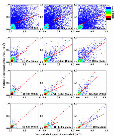
Figure 10.
Scatter plots of the vertical wind speeds (absolute values) at different temporal scales of (a–c) 1, (d–f) 10, (g–i) 30 and (j–l) 60 min by the DWL and sonic wind anemometer at 47, 140 and 280 m AGLs. The vertical data are sorted into multiple cases at an interval of 0.05 m s−1. The colorful dots represent the percentages of the ordered pairs in each case, shown specifically by the color bar to the right of (c). The dashed and solid lines are the 1:1 line and the linear regression, respectively.
Wind measurements at different scales have different meanings. On a small scale, the wind represents the variation in turbulence, whereas at the mesoscale or large scale, the wind reflects the variations in air masses. The DWL is spatially separated by about 20 m from the sonic wind anemometers. Thus, DWL is not measuring the same volume of air as the sonics. Much of the poor correlation between the sonic wind anemometer and DWL vertical motion at small timescales is due to the fact that they are sampling different portions of turbulent eddies, particularly small eddies. The vertical average along the pulse is inherent to the DWL observation, whereas the sonic wind anemometer measurement volume is only a few cubic centimetres [38]. The correlation improves with spatial time, which corresponds to the large eddies that are more coherent in space. This may explain why the results are better at high altitudes, as the maximum eddy size decreases closer to the surface; thus, the vertical wind decorrelates at shorter distances.
5.3. TKE Validation of the DWL by a Sonic Wind Anemometer
Turbulence is an important physical parameter that reflects small-scale atmospheric motions and can be calculated by the three-dimensional wind disturbance. To date, the TKE has commonly been retrieved by sonic wind anemometers, while the retrieval of the TKE by lidar needs to be further explored. Figure 11a depicts the TKE variation imaged by the DWL with PM2.5. Clearly, the TKE was spatially distributed in the planetary boundary layer. The sonic wind anemometer was fixed at a specified height near the ground, limiting its observation range. The lidar can show a spatial distribution of turbulence that is superior to that obtained by the sonic wind anemometer. Figure 11b,c show the variations in the TKE from the DWL and sonic wind anemometer below 300 m. The TKE obviously differed between the two observation instruments. The TKE obtained by the DWL changed more drastically at higher wind speeds, while the overall change in the TKE captured by the sonic wind anemometer was smoother. At lower wind speeds, the TKE trends from the DWL and sonic wind anemometer were consistent. When the aerosols changed drastically, the TKE measured by the DWL was also much higher than that measured by the sonic wind anemometer. The difference in the TKE corresponded to the vertical wind but was less associated with the horizontal wind.
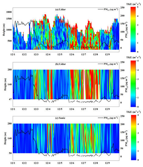
Figure 11.
Temporal hourly variations in the turbulent kinetic energy (TKE) by (a) the DWL and the TKE variations imaged by the (b) DWL and (c) sonic wind anemometer at 47, 140 and 280 m AGLs. The black line is the temporal hourly variation in PM2.5.
The vertical wind sampling frequency of the DWL is 0.05 Hz, while the sampling frequency of the sonic wind anemometer is 10 Hz. It is certainly true that lidars cannot measure eddies smaller than their sampling volume, but they can accurately measure other features that they can properly resolve. Many studies have used different lidar systems (Windcube; Halo lidars; ZephIR, etc.) with the different measurement methods (VAD; six beam method; vertical-stare mode for vertical wind speed only; pair of low-elevation RHIs for horizontal wind only, etc.) to examine whether lidar can measure turbulence, and have shown promising results compared to the sonic wind anemometer [9,35,39,40,41,42,43]. On the premise of accuracy, it is possible for lidar to measure turbulence by increasing the three-dimensional wind frequency.
Each instrument has unique advantages and disadvantages. Their difference in temporal scales is the advantages of the DWL and sonic wind anemometer, as this difference also determines the uniqueness of these sensors under varying conditions. When the retrieval assumption is not violated, the DWL can reasonably estimate the average wind conditions, but it is not good enough for turbulence. The reason is that the DWL wind retrieval method is based on the horizontal uniform wind in the scanning cone (DBS in this study), which is not the case for turbulence, especially urban wind observation. To capture large turbulent eddies, triple DWLs are required. Hence, wind measurements should be seriously considered and employed for different purposes and application scenarios.
In this validation, the performance process, precision analysis and TKE discussion of the DWL are concentrated in the polluted urban area with a strong regionality. The applicability and function of the DWL under other conditions also need to be studied. Besides, only the DBS mode of the DWL was tested in this study, whereas features of the VAD and the six-point beam method remain to be explored.
6. Conclusions
The horizontal and vertical winds measured by a DWL were systematically validated by data from the 325 m meteorological tower in the polluted urban area. In general, DWL was reliable at monitoring the three-dimensional wind with the expected spatial and temporal resolution. The three wind measurement instruments tested, namely, the DWL (Windcube 100s), cup anemometer/wind vane and sonic wind anemometer, have unique advantages and weaknesses because of the different observation principles. The cup anemometer/wind vane is the most widely used and cost-effective horizontal wind measurement instrument, whereas the sonic wind anemometer and DWL have the ability to measure three-dimensional wind and turbulence. Our comparison showed that both instruments (the DWL and sonic wind anemometer) were basically consistent. Nevertheless, the vertical wind imaged by the DWL did not agree with that obtained by the sonic wind anemometer. Due to different spatial and temporal resolutions, the three instruments showed different performances. The DWL had an advantage at obtaining high-altitude wind fields with a higher spatial resolution than those of the other instruments. However, the cup and sonic wind anemometer were located at a fixed site with limited observation heights. The sonic wind anemometer was able to output high-frequency data (10 Hz) and was thus ideally suited to the measurement of air turbulence. However, the frequencies of the DWL were less than those of the sonic wind anemometer and were better at monitoring larger turbulent eddies. It was noted that the wind difference between the DWL and meteorological tower became increasingly notable as the aerosols rapidly varied.
Author Contributions
Conceptualization, J.X.; software, Y.M. (Yongxiang Ma); validation, X.W. and D.J.; formal analysis, Y.M. (Yongjing Ma); investigation, H.Z.; resources, F.W.; data curation, L.Z.; writing—original draft preparation, L.D.; writing—review and editing, J.X. All authors have read and agreed to the published version of the manuscript.
Funding
This research was supported by the Ministry of Science and Technology of China, grant number 2016YFC0202001; the CAS Strategic Priority Research Program, grant number XDA23020301; and the National Natural Science Foundation of China, grant number 41375036.
Conflicts of Interest
The authors declare no conflict of interest.
References
- Gresham, C.A.; Williams, T.M.; Lipscomb, D.J. Hurricane Hugo Wind Damage to Southeastern U.S. Coastal Forest Tree Species. Biotropica 1991, 23, 420. [Google Scholar] [CrossRef]
- Hoogwijk, M.; Vries, B.D.; Turkenburg, W. Assessment of the global and regional geographical, technical and economic potential of onshore wind energy. Energy Econ. 2004, 27, 889–919. [Google Scholar] [CrossRef]
- Turner, A.G.; Annamalai, H. Climate change and the South Asian summer monsoon. Nat. Clim. Chang. 2012, 2, 587–595. [Google Scholar] [CrossRef]
- Novan, K. Valuing the Wind: Renewable Energy Policies and Air Pollution Avoided. Am. Econ. J. Econ. Policy 2015, 7, 287–294. [Google Scholar] [CrossRef]
- Cañadillas, B.; Westerhellweg, A. Testing the performance of a ground-based wind LiDAR system: One-year inter-comparison at the offshore platform FINO1. Dewi Mag. 2011, 38, 58–74. [Google Scholar]
- Friedrich, K.; Lundquist, J.K.; Aitken, M.; Kalina, E.A.; Marshell, R.F. Stability and Turbulence in the Atmospheric Boundary Layer: A Comparison of Remote Sensing and Tower Observations. Geophys. Res. Lett. 2012, 39, 137–149. [Google Scholar] [CrossRef]
- Lundquist, J.K.; Churchfield, M.J.; Lee, S.; Clifton, A. Quantifying error of lidar and sodar Doppler beam swinging measurements of wind turbine wakes using computational fluid dynamics. Atmos. Meas. Tech. 2015, 8, 907–920. [Google Scholar] [CrossRef]
- Haefele, A.; Ruffieux, D. Validation of the 1290 MHz wind profiler at Payerne, Switzerland, using radiosonde GPS wind measurements. Meteorol. Appl. 2015, 22, 873–878. [Google Scholar] [CrossRef]
- Sathe, A.; Mann, J. A review of turbulence measurements using ground-based wind lidars. Atmos. Meas. Tech. 2013, 7, 3147–3177. [Google Scholar] [CrossRef]
- Newman, J.F.; Klein, P.M.; Wharton, S.; Sathe, A.; Bonin, T.A.; Chilson, P.B.; Muschinski, A. Evaluation of three lidar scanning strategies for turbulence measurements. Atmos. Meas. Tech. 2017, 9. [Google Scholar]
- Lundquist, J.K.; Wilczak, J.M.; Ashton, R.; Bianco, L.; Brewer, W.A.; Choukulkar, A.; Clifton, A.; Debnath, M.Q.; Delgado, R.; Friedrich, K.; et al. Assessing State-of-the-Art Capabilities for Probing the Atmospheric Boundary Layer: The XPIA Field Campaign. Bull. Am. Meteorol. Soc. 2017, 2, 98. [Google Scholar] [CrossRef]
- Kumer, V.M.; Reuder, J.; Furevik, B.R. A Comparison of LiDAR and Radiosonde Wind Measurements. Energy Procedia 2014, 53, 214–220. [Google Scholar] [CrossRef]
- Päschke, E.; Leinweber, R.; Lehmanu, V. An one-year comparison of 482 MHz radar wind profiler, RS92-SGP Radiosonde and 1.5 μm Doppler Lidar wind measurements. Atmos. Meas. Tech. Discuss 2014, 7, 11439–11479. [Google Scholar] [CrossRef]
- Weissmann, M.; Busen, R.; Dörnbrack, A.; Rahm, S.; Reitebuch, O. Targeted Observations with an Airborne Wind Lidar. J. Atmos. Ocean. Technol. 2005, 22, 1706–1719. [Google Scholar] [CrossRef]
- Achtert, P.; Brooks, I.M.; Brooks, B.J.; Moat, B.I.; Prytherch, J.; Persson, P.O.G.; Tjernström, M. Measurement of wind profiles by motion-stabilised ship-borne Doppler lidar. Atmos. Meas. Tech. 2015, 8, 4993–5007. [Google Scholar] [CrossRef]
- Chan, C.K.; Yao, X. Air pollution in mega cities in China. Atmos. Environ. 2008, 42, 1–42. [Google Scholar] [CrossRef]
- Kan, H.D.; Chen, R.J.; Tong, S.L. Ambient air pollution, climate change, and population health in China. Environ. Int. 2012, 42, 10–19. [Google Scholar] [CrossRef]
- Huang, R.J.; Zhang, Y.L.; Bozzetti, C.; Ho, K.F.; Cao, J.J.; Han, Y.M.; Daellenbach, K.R.; Slowik, J.G.; Platt, S.M.; Canonaco, F.; et al. High secondary aerosol contribution to particulate pollution during haze events in China. Nature 2014, 514, 218–222. [Google Scholar] [CrossRef]
- He, J.J.; Gong, S.L.; Yu, Y.; Yu, L.J.; Wu, L.; Mao, H.J.; Song, C.B.; Zhao, S.P.; Lin, H.L.; Li, X.Y.; et al. Air pollution characteristics and their relation to meteorological conditions during 2014-2015 in major Chinese cities. Environ. Pollut. 2017, 223, 484–496. [Google Scholar] [CrossRef]
- Al-Jiboori, M.H.; Hu, F. Surface Roughness around a 325-m Meteorological Tower and Its Effect on Urban Turbulence. Adv. Atmos. Sci. 2015, 22, 595–705. [Google Scholar] [CrossRef]
- Zhao, D.D.; Xin, J.Y.; Gong, C.S.; Quan, J.N.; Liu, G.J.; Zhao, W.P.; Wang, Y.S.; Liu, Z.; Song, T. The formation mechanism of air pollution episodes in Beijing city: Insights into the measured feedback between aerosol radiative forcing and the atmospheric boundary layer stability. Sci. Total Environ. 2019, 692, 371–381. [Google Scholar] [PubMed]
- Li, Y.M.; Zhang, Q.H.; Ji, D.S.; Wang, T.; Wang, Y.W.; Wang, P.; Ding, L.; Jiang, G.B. Levels and Vertical Distributions of PCBs, PBDEs, and OCPs in the Atmospheric Boundary Layer: Observation from the Beijing 325-m Meteorological Tower. Environ. Sci. Technol. 2009, 43, 1030–1035. [Google Scholar] [PubMed]
- Li, Q.S.; Zhi, L.; Hu, F. Boundary layer wind structure from observations on a 325 m tower. J. Wind Eng. Ind. Aerodyn. 2010, 98, 818–832. [Google Scholar]
- Yuan, S.F.; Jiang, R.B.; Qie, X.S.; Wang, D.F.; Sun, Z.L.; Liu, M.Y. Characteristics of upward lightning on the Beijing 325 m meteorology tower and corresponding thunderstorm conditions. J. Geophys. Res. Atmos. 2017, 122, 12093–12095. [Google Scholar]
- McCaffrey, K.; Quelet, P.T.; Choukulkar, A.; Wilczak, J.M.; Wolfe, D.E.; Oncley, S.P.; Brewer, W.A.; Debnath, M.; Ashton, R.; Jungo, G.V.; et al. Identification of tower-wake distortions using sonic anemometer and lidar measurements. Atmos. Meas. Tech. 2017, 10, 393–407. [Google Scholar]
- Wieringa, J. A revaluation of the Kansas mast influence on measurements of stress and cup anemometer overspeeding. Bound.-Layer Meteorol. 1980, 18, 411–430. [Google Scholar]
- Hayashi, T. Dynamic Response of a Cup Anemometer. J. Atmos. Ocean. Technol. 1987, 4, 281–287. [Google Scholar]
- Turner, D.B. Comparison of Three Methods for Calculating the Standard Deviation of the Wind Direction. J. Appl. Meteorol. 1987, 25, 703. [Google Scholar]
- Yamartino, R.J. A Comparison of Several “Single-Pass” Estimators of the Standard Deviation of Wind Direction. J. Appl. Meteorol. 1987, 23, 1372–1377. [Google Scholar]
- Wilczak, J.M.; Oncley, S.P.; Stage, S.A. Sonic anemometer tilt correction algorithms. Bound.-Layer Meteorol. 2001, 99, 127–150. [Google Scholar]
- Kumer, V.M.; Reuder, J.; Dorninger, M.; Zauner, R.; Grubišić, V. Turbulent kinetic energy estimates from profiling wind LiDAR measurements and their potential for wind energy applications. Renew. Energy 2016, 99, 898–910. [Google Scholar] [CrossRef]
- Quan, J.; Tie, X.; Zhang, Q.; Liu, Q.; Li, X.; Gao, Y.; Zhao, D.L. Characteristics of heavy aerosol pollution during the 2012–2013 winter in Beijing, China. Atmos. Environ. 2013, 88, 83–89. [Google Scholar] [CrossRef]
- Liu, Z.; Hu, B.; Zhang, J.K.; Yu, Y.C.; Wang, Y.S. Characteristics of aerosol size distributions and chemical compositions during wintertime pollution episodes in Beijing. Atmos. Res. 2015, 168, 1–12. [Google Scholar] [CrossRef]
- Newsom, R.K.; Brewer, W.A.; Wilczak, J.M.; Wolfe, D.E.; Oncley, S.P.; Lundquist, J.K. Validating precision estimates in horizontal wind measurements from a Doppler lidar. Atmos. Meas. Tech. 2017, 10, 1229–1240. [Google Scholar] [CrossRef]
- Sathe, A.; Mann, J.; Vasiljevic, N.; Lea, G. A six-beam method to measure turbulence statistics using ground-based wind lidars. Atmos. Meas. Tech. 2015, 8, 729–740. [Google Scholar] [CrossRef]
- Ratto, G.; Maronna, R.; Berri, G. Analysis of Wind Roses Using Hierarchical Cluster and Multidimensional Scaling Analysis at La Plata, Argentina. Bound.-Layer Meteorol. 2010, 137, 477–492. [Google Scholar] [CrossRef]
- Kane, R.P. Geomagnetic field variations. Space Sci. Rev. 1976, 18, 413–540. [Google Scholar] [CrossRef]
- Bonin, T.A.; Newman, J.F.; Klein, P.M.; Chilson, P.B.; Wharton, S. Improvement of vertical velocity statistics measured by a Doppler lidar through comparison with sonic anemometer observations. Atmos. Meas. Tech. 2016, 9, 5833–5852. [Google Scholar] [CrossRef]
- Browninga, K.A.; Wexler, R. The Determination of Kinematic Properties of a Wind Field Using Doppler Radar. J. Appl. Meteorol. 1968, 7, 105–113. [Google Scholar] [CrossRef]
- Mann, J.; Cariou, J.P.; Courtney, M.S.; Parmentier, R.; Mikkelsen, T.; Wagner, R.; Lindelöw, P.; Sj¨oholm, M.; Enevoldsen, K. Comparison of 3D turbulence measurements using three staring wind lidars and a sonic anemometer. Meteorol. Ztschrift 2009, 18, 135–140. [Google Scholar] [CrossRef]
- Sathe, A.; Mann, J.; Gottschall, J.; Courtney, M.S. Can Wind Lidars Measure Turbulence? J. Atmos. Ocean. Technol. 2011, 28, 853–868. [Google Scholar] [CrossRef]
- Wang, Y.S.; Hocut, C.M.; Hoch, S.W.; Creegan, E.; Fernando, H.J.S.; Whiteman, C.D.; Felton, M.; Huynh, G. Triple doppler wind lidar observations during the mountain terrain atmospheric modeling and observations field campaign. J. Appl. Remote Sens. 2016, 10, 02615. [Google Scholar] [CrossRef]
- Fuertes, F.C.; Iungo, G.V.; Porté-Agel, F. 3D turbulence measurements using three synchronous wind lidars: Validation against sonic anemometry. J. Atmos. Ocean. Technol. 2014, 31, 1549–1556. [Google Scholar] [CrossRef]


© 2020 by the authors. Licensee MDPI, Basel, Switzerland. This article is an open access article distributed under the terms and conditions of the Creative Commons Attribution (CC BY) license (http://creativecommons.org/licenses/by/4.0/).