Article

A Fuzzy-Logic-Based Covariance Localization Method in Data Assimilation

College of Physics and Electrical Engineering, Northwest Normal University, Lanzhou 730070, China
*
Author to whom correspondence should be addressed.
Atmosphere 2020, 11(10), 1055; https://doi.org/10.3390/atmos11101055
Submission received: 12 August 2020 / Revised: 29 September 2020 / Accepted: 29 September 2020 / Published: 1 October 2020
(This article belongs to the Section Atmospheric Techniques, Instruments, and Modeling)

Abstract

:
In ensemble data assimilation systems, the impracticalities of full sampling and systematic error often lead to spurious correlations between two variables with low actual correlations. To solve these problems, researchers have previously proposed a covariance localization (CL) method, which mainly involves the Schur product between a state error covariance matrix and a distance-based correlation matrix. Although this CL method can reduce spurious correlations to a certain extent, observational data remain difficult to be used effectively, which results in unreasonable assimilation. In this study, we develop a new CL method coupled with a fuzzy logic control algorithm, which we call the covariance fuzzy (CF) method. The proposed CF method is a distance-based localization method with “fuzzy” vanishing correlations in data assimilation (DA) systems. To verify the effectiveness of the new algorithm, we conducted a set of experiments using an ensemble Kalman filter (EnKF) that combines the nonlinear Lorenz-96 model or the quasi-geostrophic (QG) models. First, the performances of the CL and CF methods are discussed with respect to different strength forcings, ensemble sizes, and covariance inflation factors. The experimental results show that the proposed CF method can obtain a more effective observation weight than the CL method and can reduce the errors caused by spurious correlations. Additionally, using power spectral density (PSD) as a performance evaluation index, the robustness of the proposed fuzzy logic localization method is demonstrated. However, the application of the fuzzy logic-based localization methodology to a real atmospheric model remains to be tested.

1. Introduction

Data assimilation (DA) engages a set of specialized techniques that combine geoscience model forecasts with available observational data to determine the best estimates of the corresponding geoscientific state. The ensemble Kalman filter (EnKF) was developed on the basis of stochastic dynamic prediction theory [1] and was first introduced to the geosciences by Evensen [2]. To restrict computational cost, real EnKF DA systems are typically implemented with small ensembles of 100 members or less [3,4,5]. However, small ensembles can cause a series of problems, including rank deficiency, distanced spurious correlations, and Monte Carlo sampling errors [6,7,8,9]. Therefore, a number of auxiliary techniques have been developed and reported in the literature, including covariance inflation, as well as localization and hybrid covariances [10,11,12,13,14].
When assimilation analysis is carried out in a DA system, for each model grid point, a local strategy is equivalent when performing the assimilation analysis within a dimensional subspace of predefined correlation length from each observation; that is, observations beyond a given distance to the model grid point have no effect on updating the analysis. Traditional localization techniques are fundamentally dependent on distance-dependent decreasing functions in DA, which not only avoid the aforementioned false correlations but also greatly reduce the computational complexity of the analysis. Hence, on the basis of the physical distance between the location of model variables and/or observations, many scholars [15,16,17] studied covariance localization in the context of the EnKF. For instance, Houtekamer and Mitchell [10] first developed a local analysis framework that updates a model variable using its neighborhood observations. To choose the Gaspari–Cohn (GC) function [18] as a cutoff function, a covariance localization (CL) scheme was computed using a Schur product [12].
To alleviate large-scale problems caused by high computer memory requirements, some alternative localization schemes have been proposed, including the cross-covariance matrix between the forecast variables and observation information, the Kalman gain matrix [11,16], and the ensemble of forecast perturbations [15]. Among the above solutions, Anderson [11] proposed a method for (1) developing an adaptive covariance localization algorithm in ensemble DA that uses a hierarchical ensemble filter, and (2) estimating localization functions to reduce sampling errors. Alternatively, one can perform localization in the observation space [19] or implement it in the context of a local EnKF [20,21,22] to reduce the size of the related matrices, normally known as domain localization (DL) in some studies. Moreover, to investigate the relationship between covariance localization and local analysis in practice, Sakov and Bertino [17] concluded that the two methods should draw similar conclusions, although CL and DL are not mathematically equivalent in general. Moreover, the choice between them should be based on other criteria such as numerical effectiveness and scalability.
Although the aforementioned localization frameworks have worked well in the context of many DA problems, there are some related issues that require brief discussion. First, most distance-based localization methods employ a unimodal tapering function (e.g., the GC function) to construct the corresponding matrices, which have difficulty “localizing” nonlocal observations that exhibit multimodal correlations with model variables in some particular cases [19,23]. In addition, in certain circumstances, model variables or the corresponding observation may not have associated physical locations, which may violate the principles of distance-based methods. Therefore, some adaptive localization methods, which may not be based on physical distances, have been proposed [14,22,24]. For instance, De La Chevrotiere and Harlim [24] proposed a data-driven method for improving the poorly estimated sample correlation by using a linear map. Later, Luo et al. [14] adopted an adaptive localization scheme that “localizes” nonlocal model variables and simulated observations through the detection of causal relations.
As a side remark, we note that one of the drawbacks of CL is that it still uses large regularized covariance matrices. In certain applications, it becomes difficult for the localization function to “localize” such observations with a reasonable distance weight. Therefore, some improved localization methods have been proposed. For instance, the relationships between the localization operator and the predictive dynamic equations were determined by several localization strategies [25]. More recently, on the basis of ensemble transform Kalman filters (ETKFs), Bai et al. [26] developed a fuzzy control function that performed a series of fuzzy inferences on the input distance variables to produce a more accurate observed weight coefficient than that of smoother covariance localization functions such as the GC function [18,27]. However, these experiments were only conducted with toy models such as the Lorenz-96 model, and the proposed methodology needs to be tested with more models. Moreover, to the best of our knowledge, fuzzy logic is a method involving imprecision and approximate reasoning [28,29], which seems to be more suitable in DA circumstances. Additionally, a fuzzy thought-based transition from absolute truth to partial truth needs to be tested in a more complicated model such as the quasi-geostrophic (QG) model.
Following the work of Bai et al. [26], which extended the fuzzy mathematics concepts to DA problems, we propose a new covariance localization method coupled with a fuzzy logic (FL) algorithm, namely, the CF method. To verify the effectiveness of the new algorithm, we conducted a series of experiments using the EnKF combined with the Lorenz-96 model and the QG models. The process of combining an FL algorithm with the localization, and the robustness of the new localization method were analyzed in detail. The setting of localization parameters greatly influences the effect of new algorithms, and this theoretical research remains a trending topic in DA [30,31]. Compared with the former methods in Bai et al. [26], the new proposed method is both relatively easy to achieve by programming and computationally efficient.
The overall arrangement of this paper is as follows: Section 2 presents the relevant assimilation background, including the EnKF, covariance localization, and new improved localization methods. In Section 3 and Section 4, the specific configurations and descriptions of the experiments are presented, respectively. Section 5 shows the results of our method applied to a realistic higher-dimensional QG model, followed by discussions and conclusions in Section 6.

2. Assimilation Background

2.1. Ensemble Kalman Filter

As an algorithm for generating approximate inferences, the EnKF uses equations similar to the traditional Kalman filter [32], which has two steps: prediction and analysis. The evolution of the state and observation of the measurements can both be assumed to be linear.
x k = M k : k 1 x k 1 + ξ k ξ k ~ N ( 0 , Q k ) .
y k o = H k x k + v k v k ~ N ( 0 , R k ) .
We define x k as the m-dimensional background state at time k, and y k o is the p-dimensional set of observations at time k. Following the notation of Ide et al. [33], the superscripts o and, later on, f and a refer to the observed, forecast, and analysis entities, respectively. In linear cases, M k : k 1 refers to an m × m dynamic operator matrix. H k is a p × m coefficient matrix from the state space to the observation space. The Gaussian noise processes ξ k and v k are independent of each other in time and space. Q k is an m × m model error covariance matrix, and R k is a p × p observation error covariance matrix. The observations are local, which is typical for many assimilation application assumptions, and the observational errors have no correlation ( R k is assumed to be diagonal in this study without loss of generality).
The minimum error-variance estimate of the i-th ensemble member of the analyzed state x i a is given by the following updated equation [34]:
x i a = x i f + K i ( y i 0 H i x i f ) ,
K i = P i f H i T ( H i P i f H i T + R i ) 1 ,
P i a = ( I K i H i ) P i f ( I K i H i ) T + K i R i K i T = ( I K i H i ) P i f ,
where K i is the traditional Kalman gain matrix, P i f is an m × m forecast-error covariance matrix, and the analysis-error covariance P i a is calculated by the introduction of observations. I is the m × m identity matrix. In the derivation of the above equation, the observation and background errors are assumed to be uncorrelated. For a given ensemble, the forecast ensemble perturbation is defined as A f = [ x 1 f x f ¯ , , x i f x f ¯ , , x n f x f ¯ ] , which is an m × n matrix, and n represents the size of the ensemble members. x f ¯ is the ensemble mean in the forecast ensemble. Then, P i f is approximated using the sample covariance from an ensemble of model forecasts. In the EnKF framework, there is no need to compute and store the full matrix P i f . Instead, P i f H T and H P i f H T are directly estimated using the ensembles.
P f = 1 n 1 i = 1 n ( x i f x f ¯ ) ( x i f x f ¯ ) T = 1 n 1 A f A f T ,
P f H T = 1 n 1 i = 1 n ( x i f x i f ¯ ) ( H x i f H x i f ¯ ) T ,
H P f H T = 1 n 1 i = 1 n ( H x i f H x i f ¯ ) ( H x i f H x i f ¯ ) T ,
where Equation (7) is used for the covariances between x f and H x f , while Equation (8) is used for the covariance of H x f with itself.

2.2. Traditional Covariance Localization (CL)

Covariance localization (CL) is recognized as a powerful framework for alleviating the impact of sampling errors in DA. A common approach to localization is to modify the ensemble forecast error covariance matrix by taking the Schur product with a distance-based correlation matrix [12,17]. In addition to increasing the rank of the modified covariance matrix, this operation also effectively dampens the pseudo-correlation between the observed position and the model state update position. Traditional CL [15] is applied to the EnKF as follows:
K i = ( ρ P i f ) H i T ( H i ( ρ P i f ) H i T + R i ) 1 ,
where ρ refers to the distance-based correlation matrix. To estimate the background error covariance matrix as closely as possible in a system with a small number of ensembles, the approximated calculation expression of the terms ( ρ P i f ) H i T and H i ( ρ P i f ) H i T in Equation (9) is adopted when the number of observations in the localization range is sufficient. Similar to Sakov and Bertino [17], the above terms can be approximated as follows:
( ρ P i f ) H i T 1 n 1 o = 1 p A f i o ( A f i o ) T H i T { o } ,
H i ( ρ P i f ) H i T 1 n 1 ( H i ˜ ρ H ˜ i T ) [ ( H i A f ) ( H i A f ) T ] ,  
where H i is the observation matrix for the i-th ensemble member. The upper wavy line of H ˜ i represents the observation matrix within a given localized range. H { o } indicates that all rows outside the o-th row are set to 0, and A f i o ( A f i o ) T / n 1 represents the local state error covariance, which is used for the corresponding observations in the assimilation process. As a common method used in DA studies, one can refer to Sakov and Bertino [17] for more detailed notations.

2.3. New Improved Covariance Localization Method: The CF Method

To eliminate the spurious correlation phenomenon caused by sampling errors when estimating the background error covariance under a small ensemble number condition, we propose a new localization method coupled with fuzzy logic in the EnKF, namely, the CF method. Figure 1 shows a schematic diagram of coupling the EnKF and FL, which reveals the behavior of DA processing and fuzzy logic control during the assimilation window.
A pseudo-code of the EnKF assimilation method with a localization algorithm is proposed in Algorithm 1, which describes a full main cycle of the localization EnKF that includes the analysis and forecast steps. Before calculating the state analysis, we ran the FL algorithm to obtain more accurate weight coefficients for local observations (see Algorithm). Then, an analysis of the CF method was performed by calculating the state error covariance matrix H P f H T and P f H T and the Kalman gain K. Next, the obtained observational weights were used to update the ensemble mean and anomalies (see Algorithm 1). Finally, the assimilated analysis values and covariance matrix were obtained to calculate the root-mean-square error (RMSE) of the state analysis. At the same time, the obtained new state estimation was taken as the background value of the next moment and returned to the assimilation model to start the next assimilation.
Algorithm 1: A cycle of the EnKF assimilation method with localization algorithm
Require: s t e p 0 is the assimilation step; initial background field matrix: x _ t r u e , E , S t a t s , A, R; allocate space for observation data: y, HE, pos. m is the ensemble size. n is the state dimension. A is the ensemble anomalies. s is the scaled innovation vector. S is the scaled ensemble observation anomalies. dx is the ensemble mean correction.
1: for step = 1,… s t e p 0 do
2:   E = rk4step (@L40, dt, x, F)
3:    x f = E 1 / m
4:    A f = E ( I 11 T / m )
5:    s = R 1 / 2 ( y H x f ) / m 1
6:    S = R 1 / 2 H A f / m 1
7:    G = ( I + S T S ) 1 S T
8:      Localization: Algorithm 2
9:    H A f H A = [ ( H A ) 1 T , , ( H A ) K T ] T
10:     K = ( ρ P f ) H T ( H ( ρ P f ) H T + R ) 1
11:     D = R 1 / 2 D ˜ / m 1 , D ˜ 1 = 0 and D ˜ D ˜ T / ( m 1 ) R , m
12:     T = G ( D S )
13:     d x K d y
14:     x f x f + d x
15:     A f A f + K ( D H A f )
16:     x a = x f + A f G s
17:     A a = A f + A f T
18: end for
Algorithm 2 is an embedded fuzzy logic process for a better output of weight with the distance between the state and the observation as the fuzzy input. One needs to calculate Euclidean distance between the observation point and the state update point using different models.
Algorithm 2: Get localization coefficients coupled with fuzzy logic control algorithm
Require:d is the Euclidean distance between the observation point and the state update point. w is the weight coefficient. c and σ represent the center and width of the Gaussian membership function, respectively. p o s o is the position of the observation points. ( x o , y o ) is the position of the state update points. nx is the model dimension. l 0 is the localization radius. s is the scale range, s = 10 / 3 l 0 . L is the fuzzy correlation coefficient matrix. ρ is the so-called localization correlation matrix. denotes the elementwise product of matrices.
/* abs is the absolute value function; hypot is the square root of sum of squares (hypotenuse). Gfuzzy refers to the local functions with fuzzy logic control; Gauss refers to the traditional Gaussian localization function; Gaspari_Cohn refers to the traditional Gaspari–Cohn (GC) localization function.*/
1: if n x 1 then
2:   Lorenz 96: d a b s ( p o s o x o )
3: else
4:   QG model: d h y p o t ( p o s o x o , p o s o y o )
5: end if
6: switch tag
7:     Case ‘Gfuzzy’
8:          d ,   w exp [ ( d c ) 2 / 2 σ 2 ]
9:          L ( d 1 × w 1 ) ( d 2 × w 2 ) ( d n × w n )
10:        w d L
11:    Case ‘Gauss’
12:        w = exp ( 0.5 × ( d / l 0 ) 2 )
13:    Case ‘Gaspari_Cohn’
14:       if d < = l 0 then
15:        w = 1 5 / 3 ( d / s ) 2 + 5 / 8 ( d / s ) 3 + 1 / 2 ( d / s ) 4 1 / 4 ( d / s ) 5
16:       else d > l 0 & d < = 2 l 0
17:        w = 2 / 3 ( d / s ) 1 + 4 5 ( d / s ) + 5 / 3 ( d / s ) 2 + 5 / 8 ( d / s ) 3 1 / 2 ( d / s ) 4 + 1 / 12 ( d / s ) 5
18:      
19: end switch
20: S w
21: H ( ρ P f ) H T S H ( ρ P f ) H T
22: ( ρ P f ) H T ( ρ P f ) H T w
23: K = ( ρ P f ) H T ( H ( ρ P f ) H T + R ) 1
The general components of an FL system include a database, fuzzy quantification, an inference mechanism, and defuzzification. The implementation process for coupling FL is as follows:
(1)
Create a fuzzy logic database
First, the structure of the fuzzy controller is determined and a single-input single-output fuzzy controller is selected. Then, the Euclidean distance dist between the observational and state update positions is selected as the input variable and the equivalent weight coefficient w is selected as the output variable.
(2)
Fuzzy quantification
In fuzzy logic methodology, a linguistic variable is defined as a variable that takes words or sentences in natural language as its values. A linguistic variable is used as a label of fuzzy subsets defined in the universe of discourse in which the variable is defined. In this case, the input and output fuzzy sets are defined, and then the input variable dist is divided into 20 fuzzy sets: the closest distance, second closest distance, …, second farthest distance, the farthest distance, abbreviated as { d i s t 1 , d i s t 2 , , d i s t 20 } . The quantification scaling factor Ke is set to 0.5. The output-variable weight coefficients w are divided into 20 fuzzy sets: {the highest weight, the higher weight… the second lowest weight, the lowest weight}, abbreviated as { w 1 , w 2 , , w 20 } . The quantification scaling factor Ku is set to 0.025. Above, Ke and Ku are two parameters in the FIS Editor of the Fuzzy Logic Toolbox of MATLAB®. After input and output quantification, the domains of dist and w are D = [0, 20] and W = [0, 1], respectively.
(3)
Define the membership function
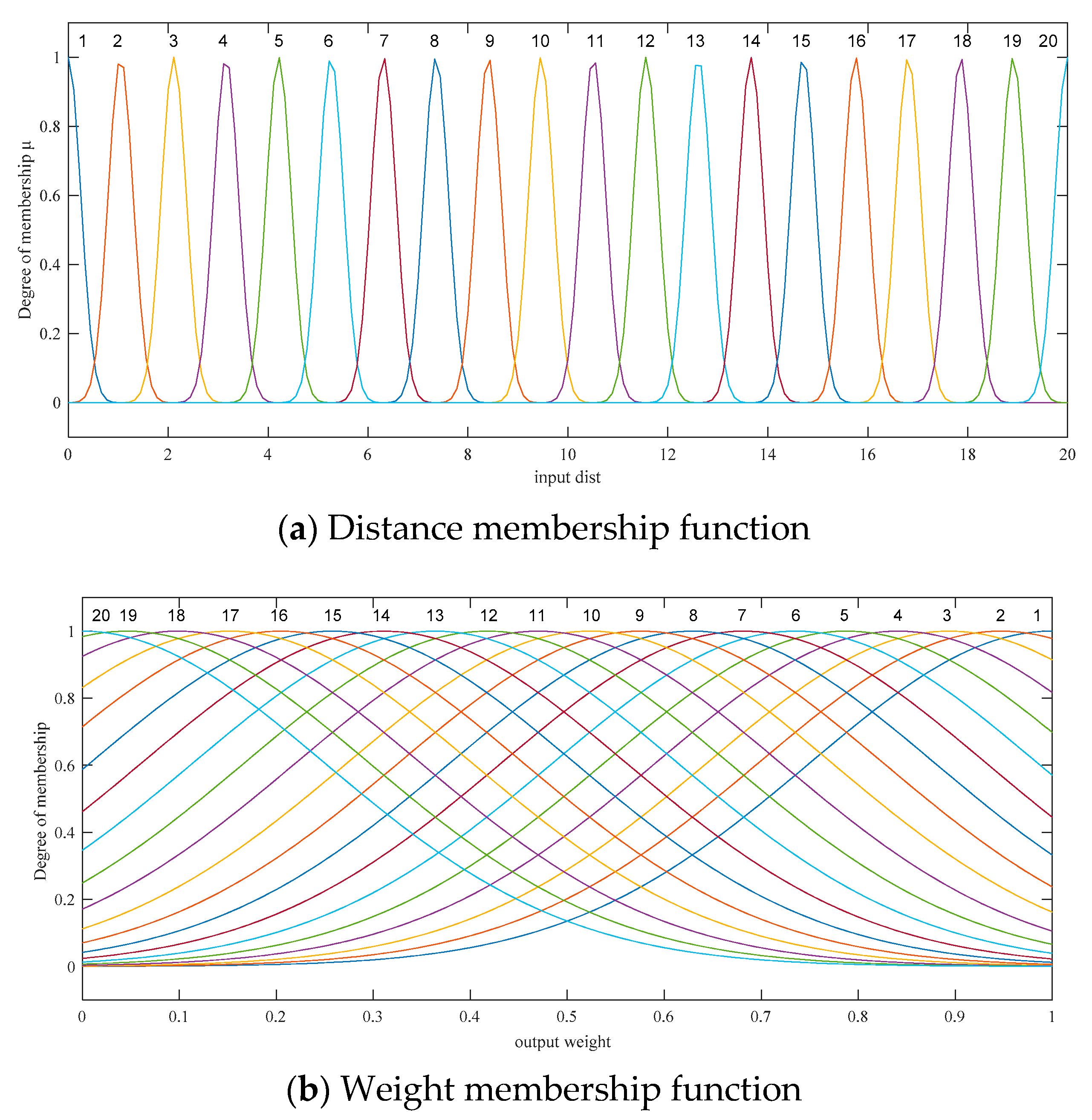
First, the Euclidean distance dist is calculated between the observation point and the corresponding state update point. On the basis of different one- or two-dimensional (1D or 2D) models, such as the Lorenz-96 model and the QG model in this study, the detailed calculation formula for the corresponding Euclidean distance is shown in the description of Algorithm 2. The distance and weight coefficient are quantified and then classified by defining the membership function. The Gaussian membership function below is given, where σ  is the standard deviation of the Gaussian distribution. Figure 2 shows the membership functions of the input and output, where σ = 0.25.
d i s t i ( d ) = { e d 2 2 σ 2 , 0 d 1 e ( d 1.5 ) 2 2 σ 2 , 1 < d 2 e ( d 20 ) 2 2 σ 2 , 19 < d 20 0 i 20 .
w i ( d ) = { e ( d 1 ) 2 2 σ 2 , 0 d 1 e ( d 0.95 ) 2 2 σ 2 , 1 < d 2 e d 2 2 σ 2 , 19 < d 20 0 i 20 .
(4)
Establish fuzzy control rules
According to the traditional experience of DA experts, with an increasing distance dist, the equivalent weight w decreases. The fuzzy inference rules are described in linguistic form below, where each rule represents the DA knowledge about how to process observational information. In this case, the set of rules below is considered and the observation meanings with “fuzzy sets” are quantified, as shown in Figure 2a (“membership functions”). Values of the membership function between 0 and 1 indicate “degrees of certainty.”
If d i s t 1 is the closest distance, then w 1 is the highest weight;
If d i s t 2 is the second closest distance, then w 2 is the higher weight;
If d i s t i is the corresponding distance, then w i is the corresponding weight;
If d i s t 19 is the second farthest distance, then w 19 is the second minimum weight;
If d i s t 20 is the farthest distance, then w 20 is the minimum weight.
L is the fuzzy relation matrix between the input and output variables, which can be expressed as a fuzzy subset on D × W . The expression is as follows:
L = ( d i s t 1 × w 1 ) ( d i s t 2 × w 2 ) ( d i s t i × w i ) ( d i s t 20 × w 20 ) ,
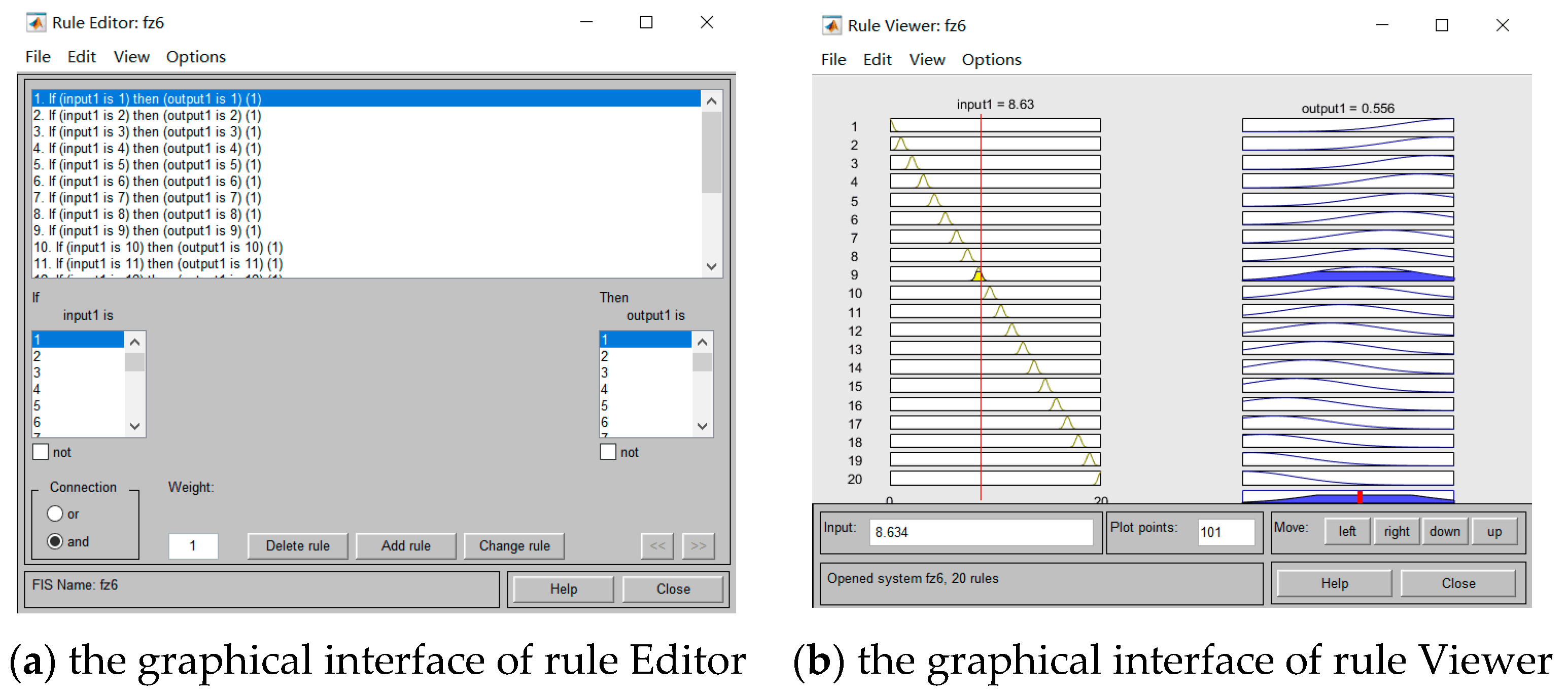
where “×” refers to the Cartesian product of the fuzzy vector. “ ” represents the union between sets. The fuzzy set operation within the rules takes the intersection, and the fuzzy set operation between the rules takes the union. Figure 3 shows the simulation result of the fuzzy rule in MATLAB.
(5)
Fuzzy inference and defuzzification
Fuzzy reasoning is the core concept of fuzzy control, which generally uses some fuzzy reasoning algorithms and fuzzy rules to obtain the final control quantity [35]. Currently, the most commonly used fuzzy inference synthesis rule is the “maximum–minimum” principle, the calculation formula for which is as follows:
w i = d i s t i L = d D ( μ d i s t i ( d ) μ L ( d ) ) / d ,
where the symbol “ ” refers to the fuzzy synthesis operation of the fuzzy vector or matrix. “ ” and “ ” are referred to as Zadeh operators, which represent large and small values, respectively. μ d i s t i ( d ) denotes the membership value of the input fuzzy distance. For example, this membership function has a value of 1 for input distance (i.e., μ d i s t ( 0 ) = 1 ), which indicates that one is absolutely certain that this value of input distance can be described as “the farthest distance”. As the input distance increases or decreases from 0, we become less certain that it can be described as “the farthest distance”. Moreover, μ L ( d ) denotes the membership value of the fuzzy relation matrix.
According to the above rules, the output control quantity w of fuzzy logic is a fuzzy quantity, which cannot be directly used to update the state in the DA system. The next step is to convert it to a precise value of execution using defuzzification methods. In general, the maximum membership degree method is employed because of its simplicity [36]. Regarding the fuzzy logic algorithm used in this study, this approach is similar to those presented in traditional intelligent control studies [37]. The choice for the membership functions or defuzzification methods can be referenced in the literature regarding different DA systems.
(6)
Model state updating
After completing the whole fuzzy logic control process, a set of weight coefficients is obtained, which is used for the next model state update. Then, we transfer the observational “fuzzy” weights obtained in this way to DA for calculating the state forecast error covariance and Kalman gain matrices, respectively. We further update the ensemble mean analysis state and anomalies through the EnKF assimilation step, obtain the analysis error RMSE at this moment, and take the updated state as the background for the next assimilation.

3. Configuration of Numerical Experiments

3.1. Experimental Model

  • The Lorenz-96 model
The Lorenz-96 model is a strongly nonlinear chaotic system with 40 state variables that can simulate the evolution of uncertain meteorological variables around a latitude circle [38]. This model has been used by many scholars as a standard for measuring the performance of DA systems. The Lorenz-96 model is described by the following second-order nonlinear differential equation with periodic boundary conditions:
d x j d t = x j + 1 x j 1 x j 2 x j 1 x j + F      j =   1 , 2 , 3 , . . . , 40 ,
where 40 variables are considered, the forcing term is F = 8, and the periodic boundary conditions are satisfied by x 1 = x 39 ,   x 0 = x 40 ,   x 41 = x 1 . A fourth-order Runge–Kutta scheme is used for temporal integration. For the experiments, we set the model time step to 0.05. A timestep of 0.05 nondimensional units in this model represents 6 h of real time, assuming that the characteristic timescale of dissipation in the atmosphere is 5 days.
b
The quasi-geostrophic (QG) model
The quasi-geostrophic (QG) model is a nonlinear model with hyper-dimensions and a relatively high model-subspace dimension. This is a simulation with a realistic atmospheric or oceanic DA system model. The QG model is a numerical approximation of the following equation with a two-dimensional vorticity field q [39]:
q t = ψ x ε J ( ψ , q ) λ Δ 3 ψ + 2 π sin ( 2 π y ) ,
where ψ may be interpreted as either a stream function or surface elevation, ε represents the frictional amplitude of the extract energy at the largest scales, and λ is the amplitude of the hyper-diffusion, which means dissipating vorticity at the smallest scales. The model domain represents a 1 × 1 square, 0 x 1 , 0 y 1 , discretized by a 129 × 129 grid with a dimension of 16,641. In this configuration, we set the timestep length to 1.25, and the background field is obtained by integrating the corresponding time step with the fourth-order Runge–Kutta scheme. At every four assimilation cycles, 300 ψ observations with an observational error variance of 4.0 are used. That is, these observations are conducted and assimilated by every four time steps, and the observed locations are symmetric and uniformly distributed in the state space. To ensure that the model simulation results are close to those of the actual ocean and atmospheric application, the selected ensemble size must be smaller than the model subspace. Therefore, all experiments using the QG model are conducted with an ensemble of 25 members.

3.2. Performance Index

In the simulated assimilation experiment, we used the RMSE and power spectral density (PSD) as indicators to evaluate the assimilation performance.
(1)
The state variables x k t and x k a are generally obtained from the numerical solutions of differential equations. The RMSE of the analysis of the ensemble mean, at the specific time k, is defined as follows:
R M S E = 1 n x ¯ k a x ¯ k t 2 ,
where the symbol “ · ” represents the norm of a vector, and x ¯ k a and x ¯ k t are the analysis and truth average values of the state variable, respectively. Normally, a better assimilation effect results in a smaller corresponding RMSE.
(2)
The power spectral density (PSD) is a probabilistic statistical value, the physical significance of which lies in the measure of the mean square value of random variables. Specifically, the area under the relation curve of the PSD–frequency value represents the variance, whereby a smaller area denotes better performance of the assimilation algorithm.
The scheme for calculating the eigenvalue of the PSD is as follows:
(i)
Given the forecast ensemble x i f , the ensemble mean x ¯ and the forecast ensemble anomalies A f = [ x 1 f x _ , , x i f x _ , , x n f x _ ] are calculated; then, the forecast covariance matrix is calculated using Equation (6).
(ii)
The analysis ensemble x i a is calculated using the Kalman analysis (see Equation (3)). Then, the analysis covariance matrix is calculated using Equation (5).
(iii)
The anomalies in the analysis ensemble and the Kalman gain are calculated.
(iv)
The eigenvalue of the PSD is calculated using the fast Fourier transform of the anomalies matrix for all ensembles A , the analyzed anomalies A a , and the forecast anomalies A f .

3.3. Experimental Design and Preliminary Results

All experiments were conducted using an EnKF-MATLAB platform developed by Sakov and Oke [40], which includes standard DA algorithms and commonly used models. In the spirit of reproducible research, we only added the fuzzy algorithms described in this article. To model the DA system behaviors, we used the Fuzzy Logic Toolbox of MATLAB® with simple logic rules and then implemented these rules in a fuzzy inference system. In addition, using the graphical user interface (GUI) editors and viewers in the Fuzzy Logic Toolbox, we could build the rules set, define the membership functions, and analyze the behavior of a fuzzy inference system (FIS).
The editors and viewers provided in the Fuzzy Logic Toolbox include an FIS Editor, Membership Function Editor, Rule Viewer, Surface Viewer, and Rule Editor. General information about the fuzzy inference system can be accessed using the FIS Editor. With the Membership Function Editor, one can display and edit the membership functions associated with the input and output variables of the FIS. For more details about using the Fuzzy Logic Toolbox, the reader is referred to the MATLAB manual. Note that this study may be considered a continuation of the work by Sakov and Bertino [17]; we used the same EnKF methods and a similar experimental design. For more details about the experimental set-ups, the reader may refer to Sakov and Bertino [17].

3.3.1. Influences of CL and CF on the Kalman Gain Matrix

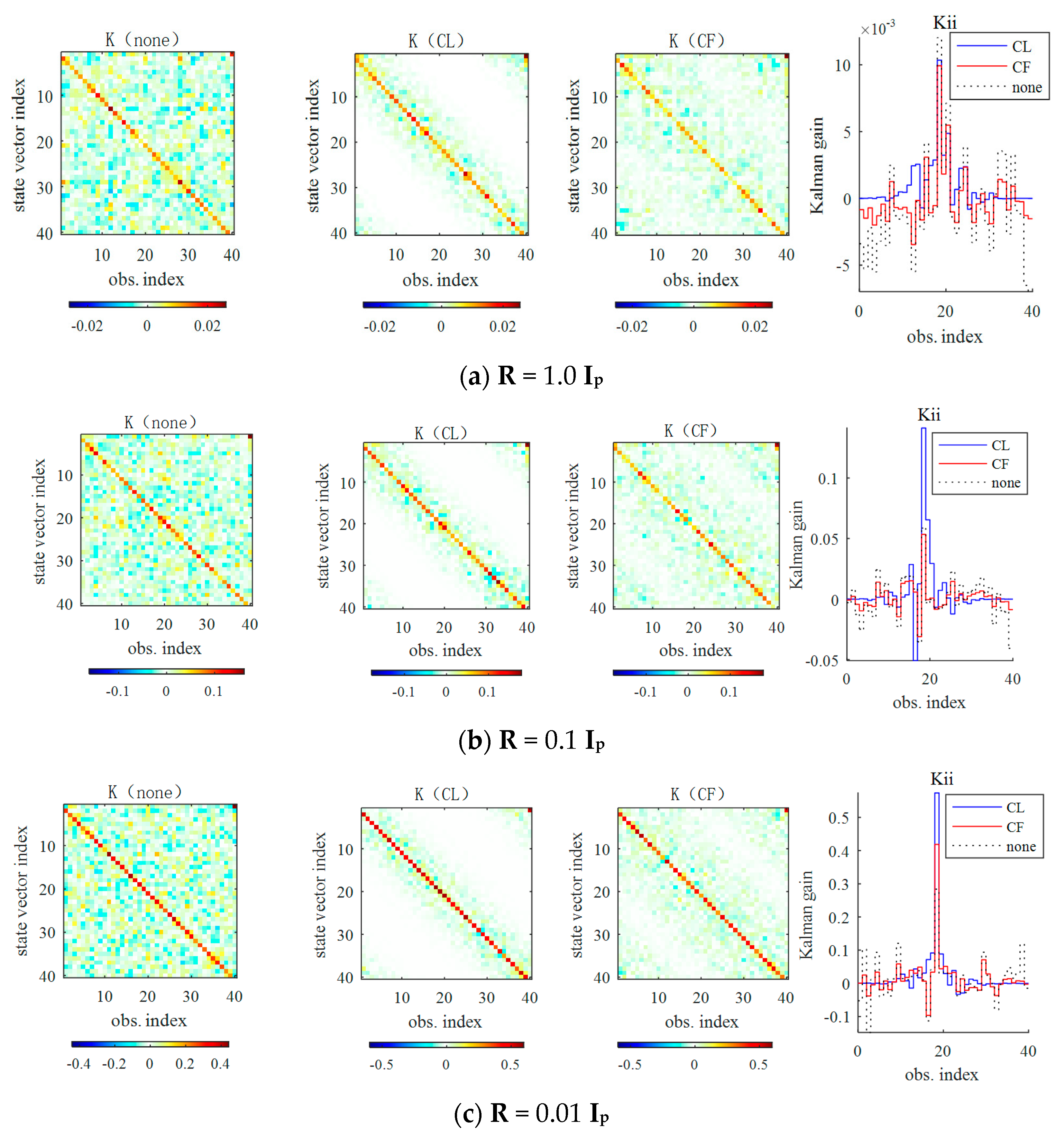
To determine the influences of CL and CF on the Kalman gain matrix K, the structure of the matrix K for different observation errors was investigated. As shown in Figure 4, “K(CF)” and “K(CL)” denote the Kalman gain with and without the fuzzy logic control, respectively, and K(none) indicates the unlocalized Kalman gain. For the three groups of experiments, we set the respective observational errors to 0.01, 0.1, and 1.0. Some parameters were set as follows in the experiment: number of ensemble members n = 20, number of observations p = 40, number of total assimilation steps = 1000, assimilation interval step = 1 time step, localization radius = 5, and covariance inflation factor = 1.08.
Figure 4 depicts the influence of CL and CF on the Kalman gain matrix. In this case, the Kalman gain was a 40 × 40 dimension matrix. The horizontal axis represents the index number of the corresponding observation vector, while the vertical axis represents the index number of state variables. Similar to Sakov and Bertino [17], we observed that the unlocalized gain matrix retains the pseudo-correlation between the states, while CL and CF both eliminate the pseudo-correlation of the long distance in the gain matrix. Another observation result is the diagonality and symmetry of the Kalman gain matrix due to the periodicity of the model. (1) In the case R = 1.0 Ip (hereafter, Ip is the p × p identity matrix), where the situation can be characterized as a “weak” assimilation according to Sakov and Bertino [17], the Kalman gains for both methods in Figure 4a produce quite different results, and there is a considerable reduction in the ensemble spread at the observation locations. The gain quickly decreases with the distance to the observation. (2) The case R = 0.1 Ip is considered an example of “moderate” data assimilation. The matrix corresponding to CL and CF is still diagonal, but the difference in Kalman gain between the two methods gradually decreases. Additionally, (3) the third row in Figure 4 shows the results for the observation error variance set as R = 0.01 Ip, which corresponds to “strong” assimilation. It can be observed that the structure of the gain matrix for CL and CF shows quite close results. The difference is reflected in those larger gains when increasing the “strength” of assimilation. Accordingly, similar experimental designs in which the Kalman gain is affected by observation errors and localization methods also appeared in Sakov and Bertino [17]. However, the difference is that two traditional localized methods, covariance localization and local analysis, were compared in Sakov and Bertino [17].

3.3.2. Comparison of the Influence on the Two Localization Methods with Different Model Errors

To compare the assimilation performance of the two localization methods under different model errors, an experiment was carried out using different values of the forcing coefficients. In this configuration, the default parameter settings were as follows: ensemble size n = 20, observational error covariance R = 1.0 Ip, number of observations p = 40, and every model time step h = 0.05. In addition, the total number of steps was 9855. To avoid adverse influences during the assimilation of transient effects, the first 1000 steps were omitted from the experiment. The experimental timeline was 365 days.
Similar to the experiment set-up in Tian et al. [41], the truth run of the Lorenz-96 model (F = 8) was used for verification and for generating observations. Another group of experiments with a moderate model error and a severe model error (incorrectly specified) was also conducted using the two different forcing coefficients F = 8.5 and F = 9.0, respectively. Figure 5 compares the performance of the two approaches with the different forcing coefficients. The experimental configurations are exactly the same as those in the ideal model space (F = 8, Figure 5a). Notably, in the presence of a moderate model error (F = 8.5, Figure 5b), it can be seen from Figure 5 that the overall RMSE of the two localization methods is relatively low, and the corresponding trend changes are similar. At F = 8.0, the average RMSEs of the CL and CF methods are the smallest (0.246 vs. 0.228), and the CF reduced RMSE by 7.3% compared with the CL. In the presence of a moderate model error (F = 8.5, Figure 5b), the CF performs moderately better than the traditional CL method (0.281 vs. 0.268), and the CF reduced RMSE by 4.6% compared with the CL. In the experiment with a severe model error (F = 9.0, Figure 5c), the performance of both localization methods is not very satisfactory (0.291 vs. 0.283) compared to other group experiments, and the CF reduced RMSE by only 2.7% compared with the CL. In conclusion, the CF approach showed better performance under the different model error scenarios. Although the effect of the CF algorithm in terms of eliminating errors was not intuitively obvious, it worked well under both perfect and imperfect model scenarios. A similar experimental design was verified in Tian et al. [41].

4. Localization Behavior Using the Lorenz-96 Model

4.1. Change in Ensemble Numbers

The selection of the number of ensemble members plays a crucial role in the DA process, which not only determines the operational efficiency of the actual assimilation system but also affects the amount of calculation required.
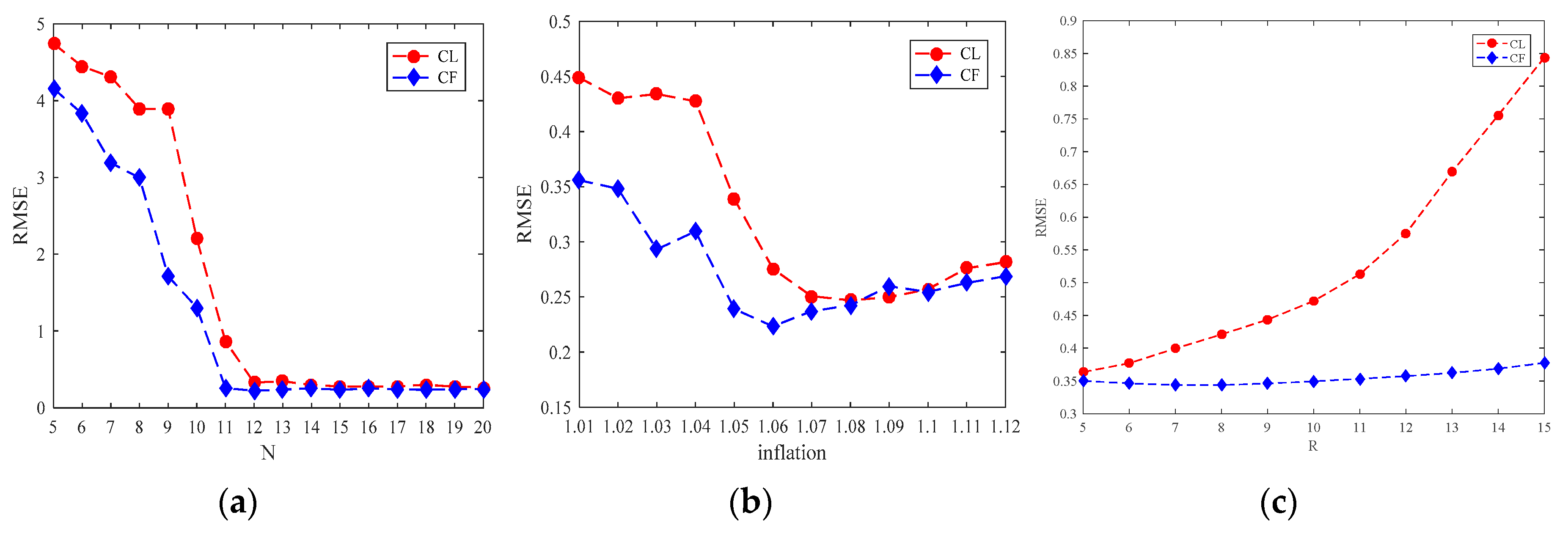
As shown in Figure 6a, for different numbers of ensemble members, the number of observations p = 40, the number of model steps T = 10, the observational error covariance R = 1.0 Ip, the inflation factor = 1.08, and the strength factor F = 8. Figure 6a shows that, for different n [ 5 , , 20 ] , the initial RMSE values of the CL algorithm are greater than those of the CF algorithm. (1) When the ensemble members increase within a certain range (0 < N ≤ 12), the analysis RMSE values of CF and CL both decrease sharply, which means that the assimilation accuracy constantly improves. However, (2) compared with CL, the analysis RMSE value of the CF method is lower, and the assimilation performance is better. (3) When the ensemble size n = 20, the two methods achieved nearly the same assimilation effect. From the above, the effectiveness of the CF algorithm was verified, and a similar experimental design was reported by Tian et al. [42].

4.2. Change in Covariance Inflation Factors

During the assimilation process, a suitable covariance inflation factor will improve the assimilation system accuracy, whereas a single inflation factor is not optimal throughout the entire model domain; to some degree, its numerical change reflects the time variation characteristics of the chaotic model. The covariance inflation factors of the selected sets vary from 1.01 to 1.12 at intervals of 0.01.
Figure 6b shows the RMSE values of the two algorithms for different inflation factors infl, which represent the average of all grid points over all time steps. In the default parameter configuration, the ensemble size n = 20, the number of observations o = 40, the model steps T = 10, the observation error covariance R = 1.0 Ip, and the forcing coefficient F = 8. The results showed that for different i n f l [ 1.01 , , 1.12 ] , the change in the RMSE value differed for each algorithm. The CF algorithm obtained the minimum RMSE error at infl = 1.06, whereas the CL algorithm obtained the minimum RMSE error at infl = 1.08. As the covariance inflation factor gradually increased, it can be seen that the fluctuation range of the CL method was larger than that of the CF method, which indicated that the localization method with the FL algorithm had strong robustness to variation in the covariance inflation factor. In addition, the change in inflation factor makes the corresponding RMSE of localization methods change rapidly, thus showing the obvious multi-peak and multi-valley phenomenon, which was taken as evidence that a genetic algorithm could be employed here as the adaptive searching method to search for an optimal inflation value within the best numerical range [43].

4.3. Change in Localization Radius

The selection of localization radius is also a key issue in data assimilation, which is not only related to its representativeness but also depends on its effective use.
The parameter settings of this experiment and fuzzy logic parameters were the same as above. Figure 6c shows the RMSE values of the two algorithms for different localizing radius. The experimental results show that the assimilation effects are different under different localizing radius, and the CF method obviously has stronger robustness and better assimilation performance than the CL method.

4.4. Performance Index PSD

In this study, we examined the performances of the CL and CF approaches using a PSD index [17]. From a mathematical point of view, the area under the PSD–frequency relationship is the variance or the square value of the response standard deviation. That is, a smaller area denotes better assimilation performance. Then, with changes in the observational error, we compared the performances of the algorithms with and without FL.
As shown in Figure 7, the “forecast” curve represents the Fourier spectrum of the ensemble singular value of the predicted values, and “CL” and “CF” denote the respective Fourier spectra of the ensemble singular values of the analytical values. Figure 7a–c correspond to the power spectral density plots in the CL and CF methods with observation errors R = 0.0001 Ip, R = 0.01 Ip, and R = 1.0 Ip, respectively. When R = 0.0001 Ip, it can be clearly seen from Figure 7a that the CF is superior to the CL. As the observation error variance R increases, the corresponding PSD value of the two localization methods also increases, and the area enclosed by the coordinate axis increases; thus, the assimilation performance decreases. By observing the CF curves in Figure 7a–c, it can be seen that the error increases and the corresponding range-ability of PSD decreases. When R = 1.0 Ip, the CF method basically coincides with the predicted PSD curve. Therefore, as the observation error increases, the advantages of CF become less obvious. With respect to the experiments with the PSD values (i.e., the CL experiment), the results were similar to those of Sakov and Bertino [17]. The similarity of the results showed that the fuzzy logic assumption can efficiently deal with spurious correlations, confirming the findings of Bai et al. [26], and that the fuzzy control methodology was an efficient strategy for improving estimations of the error covariance matrix.

5. Localization Behavior Using the Quasi-Geostrophic (QG) Model

In this section, to demonstrate that the FL algorithm can also be applied to more realistic higher-dimensional systems; we also present results obtained from a simulation with a “realistic” atmospheric or oceanic DA system model, that is, a quasi-geostrophic (QG) model, which is a nonlinear model with hyper-dimensions and a relatively high model-subspace dimension.

5.1. Comparison of Assimilation Performance of Two Localization Methods

In our experimental set-up, ensemble inflation was applied in the same way as that for the Lorenz-96 model by multiplying the analyzed ensemble anomalies by a given factor, which we set to 1.14. For localization, we used Gaussian localization and Gaussian fuzzy localization functions. The former was applied to the state error covariance matrix by means of a Schur product that multiplies each element P i , j of the covariance matrix by the factor c o e f f s i , j = exp [ 0.5 × ( d i s t i j / l 0 ) 2 ] , where d i s t i j is the horizontal distance between elements i and j in the grid space, and l 0 is the localization radius. The latter was applied in the same way as for the former; however, the factor c o e f f s i j was deduced by a series of Gaussian fuzzy controls. The experiments were conducted using the EnKF method on the basis of the QG model, where the default parameter settings were as follows: ensemble size of n = 25, number of observations p = 300, dimension of the state vector m = 16,641, observation error R = 4.0 Ip, and localization radius l 0 = 15. The assimilation experiments were run for 1000 assimilation steps.
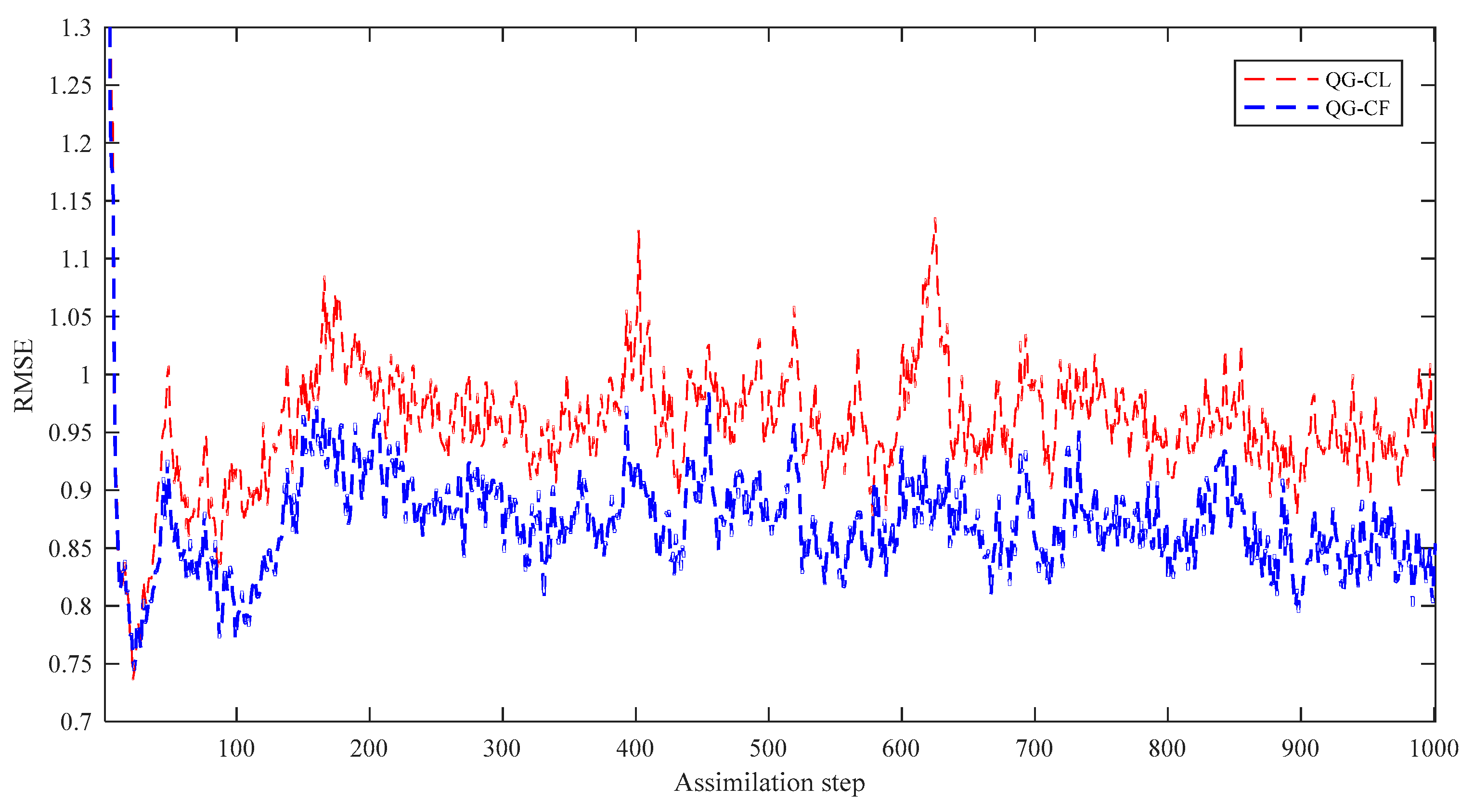
Figure 8 shows a summary of the results for the RMSE errors for the CL and CF methods using the QG model. It can be clearly seen that the overall RMSE change trends of the CF and CL methods are the same in the whole DA process without filter divergence, in accordance with the normal results [40]. Therefore, the applicability of the CF method in the QG model is demonstrated. Moreover, the performance of the CF algorithm is slightly superior to that of the traditional CL method. Numerically, the CF (RMSE = 0.8471) result is slightly smaller than that of the CL method (RMSE = 0.9464). These results are similar to those obtained with the QG model in [40]. In conclusion, the effectiveness of the new CF method is demonstrated.

5.2. Comparison of Spatial Distribution Characteristics between Two Localization Methods

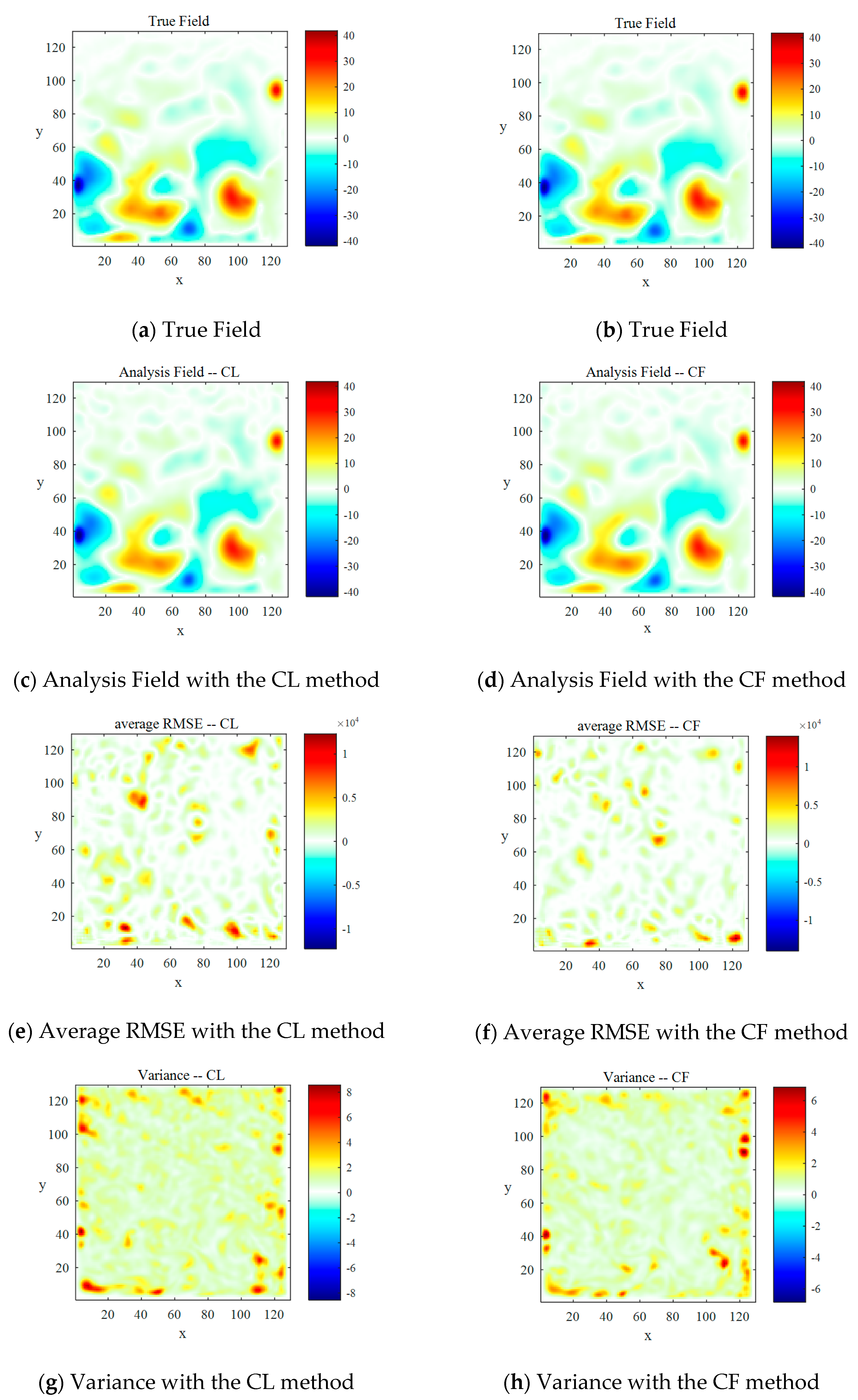
To better understand the mechanics behind fuzzy logic and check the suitability of real atmospheric systems, we compared the true field, analysis field, and error field between two different localization methods in the context of the EnKF under the QG model.
The experimental results are shown in Figure 9. The white cells correspond to the cases when the system became unstable or diverged. It can be seen from the figure that (1) the true field and the analysis field obtained by CL and CF are quantitatively similar for all systems, and the state distribution characteristics in the real assimilation system are clearly expressed; (2) according to the state distribution diagram of the average RMSE, although the performance trend of the two methods is relatively stable, it can be seen that CF is slightly better than CL. Recall that the magnitude of R is 4; it can be clearly seen that the magnitude of the errors of CF is smaller than that of CL in Figure 9. (3) From a variance distribution point of view, the most significant errors occurred along the northern boundary and were likely to be due to errors in the propagation of fast-moving waves. In addition, the variance distribution difference reflects the superiority of the CF method; (4) these results demonstrate that the two localization schemes tested here resulted in a well-constrained analysis. However, from a practical point of view, the superior performance of the CF method here may be more significant.

6. Conclusions

In this study, we proposed and tested a fuzzy logic-based covariance localization strategy using the EnKF algorithm, namely, the covariance fuzzy (CF) localization method. The purpose was to address spurious correlation problems that are usually introduced when finite ensemble members are used to estimate the background error covariance matrix. The application of this localization strategy coupling fuzzy logic algorithm moderately increased the assimilation precision while reducing the observation error. Below, we summarize this work from the following aspects:
  • Effectiveness of the new algorithm
At present, the study of the DA algorithm is mainly concerned with theoretical research, while the classic Lorenz-96 model and the QG model are often taken as the test bed [17,25]. In this study, several numerical experiments were performed with the nonlinear Lorenz-96 model and QG model, which feature a relatively high model-subspace dimension and a hyper-dimension, showing that the proposed CF method performs better than the original CL. By analyzing and comparing the changes in the Kalman gain under different observation errors, it is concluded that both methods effectively eliminate the false correlation between state variables, while the CF method is more effective in making full use of observation information to optimize assimilation analysis results.
The Wilcoxon signed rank test [44] was applied, where the symbols “+” and “−” denote that the performance of the proposed CF algorithm is better than or worse than that of the CL. As for the Lorenz-96 model experiment, there were 316 samples used for calculating the t-test. (1) At F = 8.0, there were 162 “+” and 154 “−”, which means the CF method was better than the CL method. (2) When F = 8.5, “+” and “−” both had 158, which means the algorithm proposed in this article was equivalent to the comparison algorithm. (3) At F = 9.0, there were 134 “+” and 182 “−”. This shows that the proposed algorithm performed poorly relative to the comparison algorithm at this time. (4) However, calculating a t-test with the QG model resulted in an encouraging effect. Among 1000 data, there were 989 “+” and 11 “−”. These findings show the effectiveness of the new algorithm, especially with more realistic models.
b.
Sensitivity and robustness of the new algorithm in experimental settings
To better understand fuzzy logic-based DA systems, we need to analyze the influence of the observation errors, forcing parameters, and ensemble numbers on the performance of the model. Normally, all of the parameters are fixed except for one. By doing so, the influence of the fuzzy logic methods can be studied to see how one particular parameter works. The correctness of the CF methods can be further proven with the normal toy model DA experiment, which was implemented by many scholars [17,45]. In this work, a proper selection of those parameters was expected to improve the assimilation performance of the algorithm and prevent filter divergence. By comparing the assimilation effect of the two methods under different strength forcing, ensemble numbers, and covariance inflation factors, it was found that the CF method shows strong robustness overall. The CF method may also be less susceptible to covariance inflation factors and may perform well with a smaller ensemble size than the CL method. Furthermore, inspired by Sakov and Bertino [17], we explored the robustness of the FL algorithm with respect to the use of PSD as the performance evaluation index. It was concluded that, under different observation errors, the PSD of the CF method was smaller, the variance was smaller, and the assimilation performance was better.
c.
Applicability in real weather models
To demonstrate that the fuzzy logic control algorithm can also be applied to more realistic higher-dimensional systems, we conducted experiments using the QG model. By comparing the spatial state distribution of the analysis field, the average RMSE field, and the variance field of the two methods, we found that the assimilation effect of the two methods was almost the same, but CF still had a slight advantage. Our findings indicate that, in comparison to conventional distance-based localization, fuzzy logic-based localization not only achieved close or better performance in terms of RMSE or PSD but was also more convenient to implement and use in a more practical atmospheric model. As for three-dimensional (3D) atmosphere and ocean models, one can calculate the corresponding distance according to their models and the choice of observations. For example, in Miyoshi et al. [46] accurate physical distances in the polar regions were computed and used for the localization. Future studies will focus on the algorithm’s applicability in a real model, for example, the Noah-MP land surface model, to verify its possible application in operational DA systems.
In conclusion, the experimental results presented in this work provide compelling evidence of the merits of the new CF approach in ensemble DA systems. Despite the desirability of using an FL algorithm in DA in theoretical and experimental simulations, the importance of using FL in real DA remains unclear and must be explored further in future studies.

Author Contributions

Conceptualization, X.M. and Y.B.; methodology, X.M.; validation, Y.B.; formal analysis, X.M. and L.D.; resources, Y.B.; writing—original draft preparation, Y.B.; writing—review and editing, Y.B. and L.D.; visualization, X.M.; supervision, Y.B.; funding acquisition, Y.B. All authors read and agreed to the published version of the manuscript.

Funding

This research was funded by the NSFC (National Natural Science Foundation of China) project (grant number: 41861047, 62066041, 41461078) and the Northwest Normal University Scientific research capability upgrading program (NWNU-LKQN-17-06).

Acknowledgments

We are thankful to the reviewers whose constructive comments helped significantly to improve this work.

Conflicts of Interest

The authors declare no conflict of interest.

References

  1. Epstein, E.S. Stochastic dynamic prediction. Tellus Ser. A 1969, 21, 739–759. [Google Scholar] [CrossRef]
  2. Evensen, G. Sequential data assimilation with a nonlinear quasi-geostrophic model using Monte Carlo methods to forecast error statistics. Geophys. Res. 1994, 99, 10143–10162. [Google Scholar] [CrossRef]
  3. Miyoshi, T.; Kondo, K. A multi-scale localization approach to an ensemble Kalman filter. SOLA 2013, 9, 170–173. [Google Scholar] [CrossRef] [Green Version]
  4. Roh, S.; Genton, M.G.; Jun, M.; Szunyogh, I.; Hoteit, I. Observation quality control with a robust ensemble Kalman filter. Mon. Weather Rev. 2013, 141, 4414–4428. [Google Scholar] [CrossRef] [Green Version]
  5. Nerger, L. On serial observation processing in localized ensemble Kalman filters. Mon. Weather Rev. 2015, 143, 1554–1567. [Google Scholar] [CrossRef] [Green Version]
  6. Hamill, T.M.; Anderson, J.L.; Snyder, C. Comments on Sigma-point Kalman filter data assimilation methods for strongly nonlinear systems. J. Atmos. Sci. 2009, 66, 3498–3500. [Google Scholar] [CrossRef]
  7. Anderson, J.L. Localization and sampling error correction in ensemble Kalman filter data assimilation. Mon. Weather Rev. 2012, 140, 2359–2371. [Google Scholar] [CrossRef] [Green Version]
  8. Houtekamer, P.; Zhang, F. Review of the ensemble Kalman filter for atmospheric data assimilation. Mon. Weather Rev. 2016, 144, 4489–4532. [Google Scholar] [CrossRef]
  9. Yue, M. A multiscale alignment method for ensemble filtering with displacement errors. Mon. Weather Rev. 2019, 146, 543–560. [Google Scholar]
  10. Houtekamer, P.L.; Mitchell, H.L.; Pellerin, G.; Buehner, M.; Charron, M.; Spacek, L.; Hansen, B. Atmospheric data assimilation with an ensemble Kalman filter: Results with real observations. Mon. Weather Rev. 2005, 133, 604–620. [Google Scholar] [CrossRef] [Green Version]
  11. Anderson, J.L. Exploring the need for localization in ensemble data assimilation using a hierarchical ensemble filter. Phys. D Nonlinear Phenom. 2007, 230, 99–111. [Google Scholar] [CrossRef]
  12. Hamill, T.M.; Whitaker, J.S.; Snyder, C. Distance-dependent filtering of background error covariance estimates in an ensemble Kalman filter. Mon. Weather Rev. 2001, 129, 2776–2790. [Google Scholar] [CrossRef] [Green Version]
  13. Hamill, T.M.; Snyder, C. A hybrid ensemble Kalman filter/3D-variational analysis scheme. Mon. Weather Rev. 2000, 128, 2905–2919. [Google Scholar] [CrossRef]
  14. Luo, X.; Bhakta, T.; Nævdal, G. Correlation-based adaptive Localization for ensemble based history matching methods. SPE J. 2019, 23, 396–427. [Google Scholar] [CrossRef]
  15. Houtekamer, P.L.; Mitchell, H.L. A sequential ensemble Kalman filter for atmospheric data assimilation. Mon. Weather Rev. 2001, 129, 123–137. [Google Scholar] [CrossRef]
  16. Zhang, Y.; Oliver, D.S. Improving the ensemble estimate of the Kalman gain by bootstrap sampling. Math. Geosci. 2010, 42, 327–345. [Google Scholar] [CrossRef]
  17. Sakov, P.; Bertino, L. Relation between two common localisation methods for the EnKF. Comput. Geosci. 2011, 15, 225–237. [Google Scholar] [CrossRef]
  18. Gaspari, G.; Cohn, S.E. Construction of correlation functions in two and three dimensions. Q. J. R. Meteor. Soc. 1999, 125, 723–757. [Google Scholar] [CrossRef]
  19. Fertig, E.J.; Hunt, B.R.; Ott, E.; Szunyogh, I. Assimilating non-local observations with a local ensemble Kalman filter. Tellus A 2007, 59, 719–730. [Google Scholar] [CrossRef]
  20. Ott, E.; Hunt, B.; Szunyogh, I.; Zimin, A.; Kostelich, E.; Corazza, M.; Kalnay, E.; Patiland, D.; Yorke, J. A local ensemble Kalman filter for atmospheric data assimilation. Tellus A 2004, 56, 415–428. [Google Scholar] [CrossRef]
  21. Hunt, B.R.; Kostelich, E.J.; Szunyogh, I. Efficient data assimilation for spatiotemporal chaos: A local ensemble transform Kalman filter. Phys. D 2007, 230, 112–126. [Google Scholar] [CrossRef] [Green Version]
  22. Bishop, C.H.; Hodyss, D. Flow-adaptive moderation of spurious ensemble correlations and its use in ensemble-based data assimilation. Q. J. R. Meteor. Soc. 2007, 133, 2029–2044. [Google Scholar] [CrossRef]
  23. Chen, Y.; Oliver, D.S. Levenberg-Marquardt forms of the iterative ensemble smoother for efficient history matching and uncertainty quantification. Comput. Geosci. 2013, 17, 689–703. [Google Scholar] [CrossRef]
  24. De La Chevrotière, M.; Harlim, J. A data-driven method for improving the correlation estimation in serial ensemble Kalman filters. Mon. Weather Rev. 2017, 145, 985–1001. [Google Scholar] [CrossRef] [Green Version]
  25. Bocquet, M. Localization and the iterative ensemble Kalman smoother. Q. J. R. Meteor. Soc. 2016, 142, 1075–1089. [Google Scholar] [CrossRef]
  26. Bai, Y.; Lu, Y.; Guo, P.; Ma, Y.; Ma, B. Observation error handling methods for data assimilation Coupled with fuzzy control algorithms. In Fuzzy Systems and Data Mining III; IOS Press: Amsterdam, The Netherlands, 2017; Volume 10, pp. 152–159. [Google Scholar] [CrossRef]
  27. Sakov, P.; Evensen, G.; Bertino, L. Asynchronous data assimilation with the EnKF. Tellus A 2010, 62, 24–29. [Google Scholar] [CrossRef] [Green Version]
  28. Zadeh, L.A. A Theory of Approximate Reasoning; Halstead Press: New York, NY, USA, 1979; pp. 149–194. [Google Scholar]
  29. Zadeh, L.A. Is there a need for fuzzy logic? Inf. Sci. 2008, 178, 2751–2779. [Google Scholar] [CrossRef]
  30. Flowerdew, J. Towards a theory of optimal localisation. Tellus A 2015, 67, 252–257. [Google Scholar] [CrossRef]
  31. Perianez, A.; Reich, H.; Potthast, R. Optimal Localization for Ensemble Kalman Filter systems. J. Meteorol. Soc. Jpn. 2014, 92, 585–597. [Google Scholar] [CrossRef] [Green Version]
  32. Lorenc, A.C. Analysis methods for numerical weather prediction. Q. J. R. Meteor. Soc. 1986, 112, 1177–1194. [Google Scholar] [CrossRef]
  33. Ide, K.; Courtier, P.; Ghil, M.; Lorenc, A.C. Unified notation for data assimilation: Operational, sequential, and variational. J. Meteor. Soc. Jpn. 1997, 75, 181–189. [Google Scholar] [CrossRef] [Green Version]
  34. Burgers, G.; Peter, J.V.L.; Evensen, G. Analysis scheme in the ensemble Kalman filter. Mon. Weather Rev. 1998, 126, 1719–1724. [Google Scholar] [CrossRef]
  35. Zadeh, L.A. Fuzzy logic and approximate reasoning. Syntheses 1975, 30, 407–428. [Google Scholar] [CrossRef]
  36. Passino, K.M.; Yurkovich, S. The Control Handbook. Fuzzy Control; CRC Press: Boca Raton, FL, USA, 1996; pp. 1001–1017. [Google Scholar]
  37. Siddique, N. Computational Intelligence: Synergies of Fuzzy Logic, Neural Networks and Evolutionary Computing; John Wiley & Sons Inc.: Hoboken, NJ, USA, 2013. [Google Scholar] [CrossRef]
  38. Lorenz, E.N.; Emanuel, K.A. Optimal sites for supplementary weather observations: Simulation with a small model. Atmos. Sci. 1998, 55, 399–414. [Google Scholar] [CrossRef]
  39. Jelloul, M.B.; Huck, T. Basin-mode interactions and selection by the mean flow in a reduced-gravity quasigeostrophic model. J. Phys. Oceanogr. 2003, 33, 2320–2332. [Google Scholar] [CrossRef]
  40. Sakov, P.; Oke, P.R. A deterministic formulation of the ensemble Kalman filter: An alternative to ensemble square root filter. Tellus A 2008, 60, 361–371. [Google Scholar] [CrossRef] [Green Version]
  41. Tian, X.; Xie, Z.; Sun, Q. A POD-based ensemble four-dimensional variational assimilation method. Tellus A 2011, 63, 805–816. [Google Scholar] [CrossRef]
  42. Tian, X.; Zhang, H.; Feng, X.; Xie, Y. Nonlinear Least Squares En4DVar to 4DEnVar Methods for Data Assimilation: Formulation, Analysis, and Preliminary Evaluation. Mon. Weather Rev. 2018, 146, 77–93. [Google Scholar] [CrossRef]
  43. Bai, Y.; Li, X. Evolutionary Algorithm-Based Error Parameterization Methods for Data Assimilation. Mon. Weather Rev. 2011, 139, 2668–2685. [Google Scholar] [CrossRef] [Green Version]
  44. Derrac, J.; García, S.; Molina, D.; Herrera, F. A practical tutorial on the use of nonparametric statistical tests as a methodology for comparing evolutionary and swarm intelligence algorithms. Swarm Evol. Comput. 2011, 1, 3–18. [Google Scholar] [CrossRef]
  45. Kalnay, E.; Li, H.; Miyoshi, T.; Yang, S.C.; Ballabera-Poy, J. 4DVar or ensemble Kalman filter? Tellus A 2007, 59, 758–773. [Google Scholar] [CrossRef] [Green Version]
  46. Miyoshi, T.; Yamane, S.; Enomoto, T. Localizing the Error Covariance by Physical Distances within a Local Ensemble Transform Kalman Filter (LETKF). SOLA 2007, 3, 89–92. [Google Scholar] [CrossRef] [Green Version]
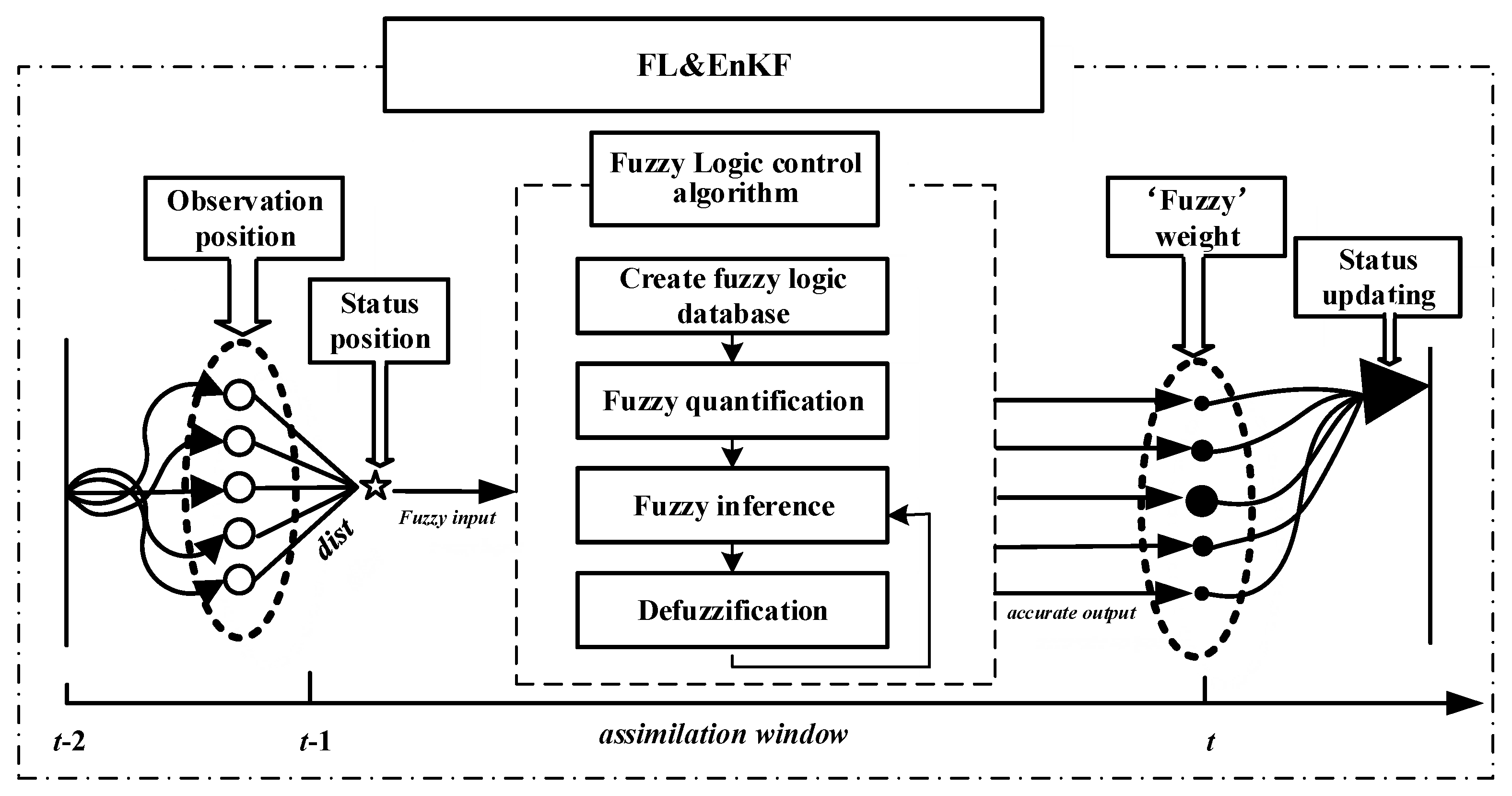
Figure 1. Schematic diagram of coupling the data assimilation algorithm with fuzzy logic (FL). Circles represent observational data, pentagrams represent status update points for the model state, and the sizes of the black dots indicate “fuzzy” weighted observations.
Atmosphere 11 01055 g001
Figure 2. Simulation diagram of the input distance and output weight fuzzy variable membership function.
Atmosphere 11 01055 g002
Figure 3. Diagram of simulation result of fuzzy rules.
Atmosphere 11 01055 g003
Figure 4. Influences of covariance localization (CL) and covariance fuzzy (CF) on the Kalman gain matrix for element i = 20 of the state vector; “K(none)” denotes the unlocalized Kalman gain. “K(CF)” and “K(CL)” denote the Kalman gain with and without the FL, respectively. “Kii” shows the gain from each observation for both methods, as well as for the case with no localization. For the three groups of experiments, the observation error variance were set to 0.01, 0.1, and 1.0.
Atmosphere 11 01055 g004
Figure 5. The daily averaged root-mean-square error (RMSE) errors of the CF and original CL methods with Lorenz-96 model in 365 simulated days (a) without a model error (F = 8.0), (b) with a moderate model error (F = 8.5), and (c) with a severe model error (F = 9.0), respectively.
Atmosphere 11 01055 g005aAtmosphere 11 01055 g005b
Figure 6. Comparison of convergence for the CL and CF with the Lorenz-96 model in different conditions: (a) the mean RMSE for a given ensemble size; (b) the mean RMSE for a given covariance inflation factor; (c) the mean RMSE for a given localization length scale.
Atmosphere 11 01055 g006
Figure 7. Power spectral density (PSD) evaluation of the CL and CF algorithms by the effect of fuzzy control. The “forecast” curve in the graph represents the Fourier spectrum of the ensemble singular values of the predicted values. “CL” and “CF” denote the Fourier spectrum of the ensemble singular values of the analytical values. For the three groups of experiments, the observation error variances were set to 0.0001, 0.01, and 1.0.
Atmosphere 11 01055 g007
Figure 8. Comparison of the RMSE mean value of each assimilation step for all grid performances of the traditional CL method and the new CF method, using the quasi-geostrophic (QG) model with the EnKF assimilation method.
Atmosphere 11 01055 g008
Figure 9. Snapshot of the spatial state distribution of the CL and CF methods at the initial truth field and the analysis field and error field at the end of the assimilation, which were run with the QG model using EnKF assimilation. The whole model localization domain was discretized by a 129 × 129 grid, with the timestep length of 1.25 and observations of 300.
Atmosphere 11 01055 g009