Abstract
This paper reviews the evolution of planetary boundary layer (PBL) parameterization schemes that have been used in the operational version of the Hurricane Weather Research and Forecasting (HWRF) model since 2011. Idealized simulations are then used to evaluate the effects of different PBL schemes on hurricane structure and intensity. The original Global Forecast System (GFS) PBL scheme in the 2011 version of HWRF produces the weakest storm, while a modified GFS scheme using a wind-speed dependent parameterization of vertical eddy diffusivity (Km) produces the strongest storm. The subsequent version of the hybrid eddy diffusivity and mass flux scheme (EDMF) used in HWRF also produces a strong storm, similar to the version using the wind-speed dependent Km. Both the intensity change rate and maximum intensity of the simulated storms vary with different PBL schemes, mainly due to differences in the parameterization of Km. The smaller the Km in the PBL scheme, the faster a storm tends to intensify. Differences in hurricane PBL height, convergence, inflow angle, warm-core structure, distribution of deep convection, and agradient force in these simulations are also examined. Compared to dropsonde and Doppler radar composites, improvements in the kinematic structure are found in simulations using the wind-speed dependent Km and modified EDMF schemes relative to those with earlier versions of the PBL schemes in HWRF. However, the upper boundary layer in all simulations is much cooler and drier than that in dropsonde observations. This model deficiency needs to be considered and corrected in future model physics upgrades.
1. Introduction
Previous theoretical studies have pointed out the important role of physical processes in the planetary boundary layer (PBL) in governing tropical cyclone (TC) intensification and maximum intensity [1,2,3,4,5,6,7,8,9,10,11]. These processes include air–sea turbulent transfer of momentum and enthalpy, turbulent mixing, convergence of absolute angular momentum (M), and boundary-layer recovery. In TC forecast models, small-scale processes such as turbulent diffusion must be parameterized, given that the horizontal grid spacing of current operational models is 2 km or coarser. Research models that are used to simulate TC intensity and structure often have horizontal grid spacing of 0.5–3 km, while scales of turbulent eddies may be as small as 10–100 m. Even with large eddy simulations that can achieve 10–100 m horizontal grid spacing [12,13,14], the lowest boundary condition still requires a parameterization of drag coefficient that is uncertain in hurricane force wind conditions [15,16]. Thus, it is important to improve turbulence parameterizations in TC models.
The sensitivity of simulated and forecasted TC intensity and structure to PBL parameterizations has been previously investigated by several studies. Most previous research has used research models, such as the fifth-generation Pennsylvania State/National Center for Atmospheric Research (NCAR) model [17,18], the Weather Research and Forecasting (WRF) model [19,20,21], the Cloud Model version 1 (CM1) [22,23], and a TC boundary-layer model [24].
As a result of the Hurricane Forecast Improvement Program (HFIP), considerable efforts have been made to upgrade the operational TC models and advance their skill for track and intensity forecasts [25]. Due to the improved performance of the Hurricane Weather and Research Forecast (HWRF) model for TC intensity forecasts, researchers have recently gained confidence in this model and started to use it to study TC processes and dynamics [26,27,28,29,30,31,32,33,34].
The HWRF model has been continuously upgraded each year, such that certain physics and initialization packages can be different from year to year. It is believed that the research community would benefit from a review of the changes that have been made to the HWRF model physics in recent years, so that when HWRF is used in research studies, the limitations and advantages of the model physics in a particular HWRF version being used are readily apparent. This study aims to review the differences in the PBL schemes used in 2011 and later versions of the operational HWRF model and assess their impacts on simulated TC intensity and structure. To evaluate contributions only from the PBL physics to the variations of TC intensity and structure, we analyze the idealized HWRF simulations using the same version of the model but with different PBL schemes and compare modeled TC structures to observations. This study aims to identify model deficiencies in terms of simulated TC structure that might be tied to the PBL physics and provide feedback to model developers for further improvements. A brief description of these PBL schemes is given in Section 2. Section 3 presents analysis of idealized simulations with these PBL schemes with a focus on evaluating the effects of the PBL schemes on hurricane structure. Structural metrics based on observational data are used in model diagnostics. This is followed by discussion and conclusions.
2. Review of PBL Schemes in the Operational HWRF
The HWRF system was initially developed at the Environmental Modeling Center (EMC) of the National Weather Service (NWS). During the past eight years, joint development of HWRF was also accomplished at several institutions, including the Hurricane Research Division (HRD), Earth System Research Laboratory (ESRL), the State University of New York at Albany, and the Developmental Testbed Center (DTC), in collaboration with EMC as part of HFIP. Below we review the PBL schemes used in recent versions of the operational HWRF model in chronological order. Table 1 summarizes the differences in these PBL schemes.

Table 1.
Summary of the main differences in different versions of the planetary boundary layer (PBL) schemes in Hurricane Weather Research and Forecasting model (HWRF). GFS denotes Global Forecast System and EDMF denotes eddy diffusivity and mass flux.
The original PBL scheme used in the 2011 (V3.4) and prior versions of HWRF is the Global Forecast System (GFS) scheme (referred to as PBL11 hereafter), which is similar to the Medium Range Forecast (MRF) scheme developed by Troen and Mahrt [35]. This scheme was implemented at the National Centers for Environmental Prediction (NCEP) in the operational GFS and later in HWRF by Han and Pan [36]. Turbulent fluxes are parameterized using the vertical eddy diffusivity and vertical gradients of mean variables in the form of:
where A is a parameter such as the wind velocity component, temperature and humidity, K is the vertical eddy diffusivity, N is the nonlocal turbulent mixing term [35], the prime represents turbulent fluctuation, and the overbar represents time average.
In PBL11, the vertical eddy diffusivity of momentum (Km) was parameterized using a parabolic equation:
where κ = 0.4 is the Von Kármán constant, u* is the friction velocity, S is the surface layer stability function, z is the height, and h is the PBL height that is defined based on a critical Richardson number.
Km = κ (u*/S) z (1 − z/h)2,
In the 2012 version of HWRF (V3.5), Km in the PBL scheme (referred to as PBL12 hereafter) was modified based on in-situ aircraft data [26,37]. A tuning parameter α was added to Equation (1) to control the magnitude and shape of Km in the form of:
Km = k (u*/S) z {α (1 − z/h) 2}.
Here, α was set to 0.5 based on extensive tests using retrospective TC forecasts [38]. The critical Richardson number was also reduced from 0.5 to 0.25 in PBL12. Zhang et al. [39] evaluated the resulting improvements in track, intensity and structure forecasts purely due to the change in α from 1 to 0.5 by analyzing over 100 retrospective HWRF forecasts. They found that lowering Km in the PBL scheme of 2012 version operational HWRF decreased 5–15% of the track and absolute intensity errors.
The PBL scheme in the 2013 and 2014 versions of HWRF (V3.6, referred to as PBL13–14 hereafter) was modified from PBL12 with two changes: (1) α was changed to 0.7 and (2) the critical Richardson number calculation was modified so that it varied with the surface Rossby number. The PBL scheme in the 2015 version of HWRF (V3.7, referred to as PBL15 hereafter) was developed in the context of improving the representation of Km by modifying α. In PBL15, α was formulated as a function of wind speed. This change was described by Bu et al. [40].
The PBL scheme used in the 2016 to 2019 versions of HWRF (V3.8–V4.0, referred to as PBL16–19 hereafter) is a different type of PBL scheme from previous versions. This scheme is a modified version of the hybrid Eddy Diffusivity Mass Flux (EDMF) scheme first implemented in the GFS model [41]. Turbulent fluxes in this scheme are parameterized using both the eddy diffusivity and mass-flux approaches in the form of:
where M is the convective mass flux and subscript up represents strong updrafts. The updraft properties are parameterized using an entrainment plume model with a lateral entrainment rate. Details of parameterizations of the mass flux and updraft velocity can be referred to in Han et al. [41]. The modification follows the work conducted in modifying Km in previous versions of the HWRF model, i.e., the α parameter in Equation (3). Besides the wind dependent setup of α as in PBL15, α is also formulated as a function of height in the PBL [42]. The mass flux component of the flux parameterization in the original GFS EDMF scheme is the same as that in HWRF.
Figure 1 compares the azimuthally averaged Km (<Km>) during the TC spin-up or intensification period in idealized HWRF simulations with the aforementioned five different PBL schemes as a function of radius and height. The maximum <Km> is located below 600 m in all simulations, and the value of the maximum <Km> is the largest in PBL11 and smallest in PBL15. The height at which <Km> is close to 0 is also largest in PBL11, indicating the boundary layer is the deepest in simulated TC by PBL11. The radial location of the maximum <Km> also varies in these simulations, which is largest in PBL11 and smallest in PBL15 (Figure 1f). This difference is tied to the storm size difference. It will be shown later that the larger simulated TC vortex is associated with smaller <Km>.
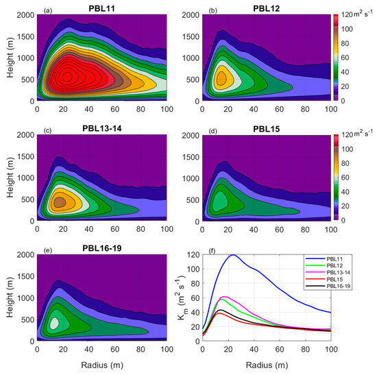
Figure 1.
Radius-height plots of the azimuthally averaged vertical eddy diffusivity (<Km>) during the rapid intensification (RI) period (t = 12–30 h) in the idealized HWRF simulations with (a) PBL11, (b) PBL12, (c) PBL13–14, (d) PBL15, and (e) PBL16–19 schemes. Radial profiles of Km averaged within the lowest 1 km layer during the RI period are shown in (f). The contour interval in (a–e) is 10 m2 s−1.
3. Results
To study the effects of different versions of the HWRF PBL schemes on hurricane intensity and structure, we ran a series of idealized simulations. These idealized simulations used the same initial vortex and boundary conditions. Except for the PBL scheme, the same HWRF code (v3.9) was used in each simulation so that the effects of the PBL scheme changes were isolated from those of other modeling system upgrades. This setup made the experiment design unique in that the findings on the sensitivity of the simulated TC intensity and structure are only from the PBL scheme.
Details of the idealized HWRF model used in this study are documented by Biswas et al. [43]. Triple domains with horizontal grid spacings of 18, 6 and 2 km are used in the configuration with no land in any domain. The environmental temperature and moisture fields are prescribed based on Jordan’s sounding [44]. The sea surface temperature is held constant at 302 K. The initial vortex is based on the method of Wang [45], in which the nonlinear balance equations in the pressure-sigma coordinate system are solved. The initial vortex strength is 20 ms−1 and the radius of the maximum wind speed (RMW) is 90 km in all simulations. Note that the decay rate of the vortex radial profile outside the RMW is similar to that in the Holland wind profile model [45]. The idealized simulations are conducted on an f-plane that is centered at 22.5° N. Besides the PBL schemes described in Section 2, other atmospheric physics options are the same as in the operational HWRF system. Grid-scale microphysical processes in the atmosphere are parameterized using the Ferrier–Aligo scheme [46]. The Scale-Aware Simplified Arakawa–Schubert (SASAS) scheme [33,47] is used to parameterize cumulus convection. The modified longwave and shortwave schemes based on the Rapid Radiative Transfer Model for General Circulation Models (RRTMG) [48] were used for radiation parameterization. In the surface layer scheme, the drag coefficient follows the COARE algorithm V3.5 in low-moderate wind conditions [49] and is fitted to available observations in high wind conditions [43]. The exchange coefficient for enthalpy transfer is configured based on the COARE V3.0 algorithm and available observations [43].
Figure 2 shows the simulated intensity in terms of maximum surface wind speed (VMAX) and minimum sea level pressure (MSLP) from five numerical experiments that used different PBL schemes described in Section 2. It is evident from Figure 2 that there is a cluster of weaker storms (PBL11, PBL13–14) and a separate cluster of stronger ones (PBL12, PBL15, PBL16–19). The storm in PBL11 is the weakest while the storm in PBL15 is the strongest at the end of the five-day simulations.
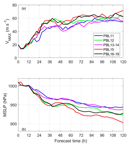
Figure 2.
Time series of storm intensity in terms of (a) maximum surface wind speed (VMAX) and (b) minimum sea level pressure (MSLP) in the five idealized HWRF simulations with different PBL schemes.
Indicated by the intensity traces, the intensification rate is also the largest in the first 36 h of the forecast period in PBL15, while it is the smallest in PBL11. The storm in PBL13–14 is the second weakest, which is followed by PBL12 and PBL16–19. The intensification rate is similar for PBL12, PBL15 and PBL16–19 during the rapid intensification (RI) period (12–30 h) in the VMAX plots (Figure 2a). The intensification rate difference during the RI period is clearer in the time series of MSLP than in VMAX (Figure 2a,b), because the MSLP varies more smoothly than the VMAX.
The maximum azimuthally averaged tangential wind speed (<v>) is another measure of storm intensity and is often used in idealized simulations to quantify storm intensity [26]. Using this metric, the difference in intensification rate is seen much more clearly than when using Vmax as the intensity metric. It is shown in Figure 3a that, during the RI period (12–30 h), the intensification rate measured by <v> in PBL11 is the smallest, while it is the largest in PBL15. The magnitude of the peak azimuthally averaged radial velocity correlates well with the maximum axisymmetric tangential wind speed (Figure 3b). The strength of the peak inflow in PBL15 is nearly three times stronger than that in PBL11.
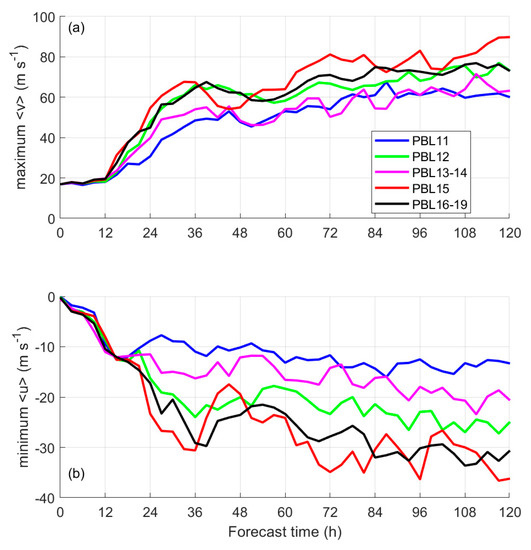
Figure 3.
Time series of (a) maximum azimuthally averaged tangential wind speed (<v>max) and (b) minimum azimuthally averaged radial wind speed (<u>min) in the five idealized HWRF simulations with different PBL schemes.
The radius of the maximum wind speed (RMW) in these simulations is also different, which is smaller when <Km> is smaller (Figure 4). The maximum azimuthally averaged 10 m wind speed (<WS10m>) is the largest in PBL15, while it is the smallest in PBL11. This result is consistent with that of VMAX, again suggesting a negative correlation between the storm intensity and Km. Note that the wind field outside the radius of 50 km is similar in all simulations except that the wind speed is slightly larger in PBL11 than in other simulations.
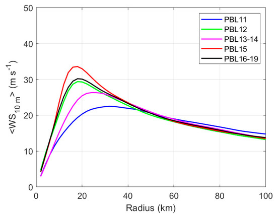
Figure 4.
Radial profiles of the azimuthally averaged wind speed at 10 m altitude (<WS10m>) during the rapid intensification period (t = 12–30 h) in the five idealized HWRF simulations.
We now evaluate the structural differences between the simulations in comparison with observational composites from Zhang et al. [50]. These composites were created using data from a total of ~800 dropsondes in 13 hurricanes. Previous studies have used these composites to evaluate TC structure from different models: a WRF-Advanced Research WRF (ARW)-simulated hurricane nature run [51], CM1 simulations [22], and TC boundary layer simulations [52,53]. These composites were also used as initial conditions in TC models simulating boundary layer rolls [46]. When evaluating the modeled structure such as the PBL height, we normalize the magnitudes of the tangential and radial wind velocities by their maximum magnitudes (c.f., Figure 3) to reduce the influence of differing simulated storm intensities [39]. All the fields are presented as functions of radius normalized by the RMW to reduce the effects of differences in storm size.
Figure 5 shows that the general structure of tangential wind speed is captured by all five simulations, including the core of strongest wind speed at the eyewall (r/RMW = 1) that is located at 600–800 m altitude. The observed radial variation of the height of the strongest wind (i.e., hvmax) is also generally captured by the simulations, showing that this height generally increases with radius. Outside the eyewall, hvmax is the largest in PBL11, which is nearly twice that of the observed value. By contrast, hvmax values in both PBL15 and PBL16–19 are close to that in the dropsonde composite (within 0–400 m). The value of hvmax in PBL12 and PBL13–14 is reduced from that in PBL11, but it is still ~300–700 m higher than in the observations.
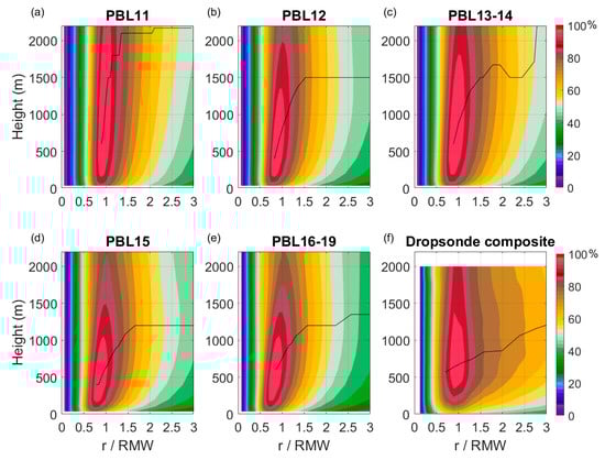
Figure 5.
Normalized radius-height plot of the azimuthally averaged tangential wind speed normalized by its maximum value (<v>/<v>max) over t = 84–108 h in the idealized HWRF simulations with (a) PBL11, (b) PBL12, (c) PBL13–14, (d) PBL15, and (e) PBL16–19 schemes. The dropsonde composite of <v>/<v>max is shown in (f). The black line denotes the height of the maximum tangential wind speed. RMW is the radius of the maximum wind speed.
The inflow layer structure from the simulations is compared to the dropsonde composite in Figure 6. Again, the radial velocity shown here is normalized by the maximum inflow strength in a similar manner as the tangential velocity to consider the difference due to the storm intensity in each simulation. The black line in Figure 6 shows the inflow layer depth, which is defined as the height at which the radial wind speed reaches 10% of its maximum magnitude [50]. As pointed out by Smith et al. [6], the inflow layer depth may be a better scale to represent the top of the PBL given its continuous variation and its dynamical constraint on TC intensification. All simulations generally captured the radial variation of the inflow layer depth outside the eyewall. However, PBL15 and PBL16–19 performed best among the experiments in the representation of the inflow layer depth, in comparison to the dropsonde composite. PBL11 is the least successful at simulating the observed inflow layer depth, while PBL12 and PBL13–14 are slightly improved from PBL11. Note that the inflow strength outside two times RMW in the dropsonde composite is much stronger than that in almost all simulations (Figure 6), which may be due to the broader vortex in the dropsonde composite (Figure 5f). Given that the shape of the radial profile of the tangential wind speed outside a 40 km radius (i.e., ~2 times RMW) is nearly the same in all simulations (Figure 5), it is worthwhile to investigate how Km affects the radial inflow structure in simulations with different initial radial vortex profiles in future studies.
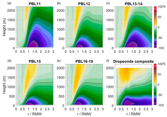
Figure 6.
Normalized radius-height plot of the azimuthally averaged radial wind speed normalized by the peak inflow strength (<u>/|<u>min|) over t = 84–108 h in the idealized HWRF simulations with (a) PBL11, (b) PBL12, (c) PBL13–14, (d) PBL15, and (e) PBL16–19 schemes. The dropsonde composite of <u>/|<u>min| is shown in (f). The black line denotes the inflow layer depth. RMW is the radius of the maximum wind speed. Negative value of u represents inflow.
The inflow angle, which represents the relative strength of radial and tangential wind velocities, is compared among the simulations with different PBL schemes and dropsonde composites near the surface (z = 10 m) in Figure 7. Again, the azimuthally averaged values are compared here. The magnitude of the maximum surface inflow angle is the smallest in PBL11, while it is the largest in PBL15. The maximum axisymmetric surface inflow angle is correlated with maximum <Km> in these simulations. This result is consistent with that of Zhang et al. [39], although they only compared two sets of HWRF real-case forecasts with PBL11 and PBL12. The simulated surface inflow angle in PBL15 and PBL16–19 simulations is closest to dropsonde observations among these simulations, indicating significant improvements in the simulated surface layer kinematic structure in the past 5 years. Note that the inflow angle magnitude in all simulations is significantly smaller than that in the dropsonde composite at and inside the radius of 0.75 times the RMW, which may be associated with the coupling problem of surface layer and boundary layer schemes in HWRF due to the tuning method [39,42]. Note also that the bin-width used in the dropsonde composite is larger than that in the average of the modeled field due to the limited horizontal resolution of the dropsonde data.
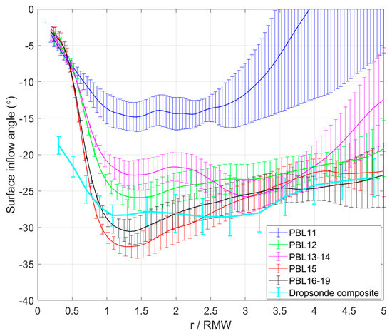
Figure 7.
Plots of the azimuthally averaged surface inflow angle as a function of radius that is normalized by the radius of maximum wind speed (RMW) in the five idealized HWRF simulations. The dropsonde composite of the surface inflow angle is also shown. The error bar represents the 95% confidence interval.
The simulated and observed thermodynamic PBL heights (zi) are also compared (Figure 8). We define zi as the height at which the vertical gradient of virtual potential temperature (θv) is 3 K/km [50]. All simulations captured the increasing trend of zi with radius outside the eyewall. The radial variation of zi inside the RMW is not seen in the dropsonde composite, which may be due to the limited horizontal resolution of the dropsonde composite. zi in PBL11 is the highest among the five experiments, while it is generally similar in the other four experiments and it is ~200 m higher than in the observations. The stability in the surface layer (<200 m altitude) varies from simulation to simulation. The surface layer is more unstable in PBL15 and PBL16–19 than in the other three simulations, while it is most stable in PBL11. Above the mixed layer, only PBL16–19 captured the strong stable layer inside the RMW, which may be related to the downward reflection of the warm core in PBL16–19 shown later.
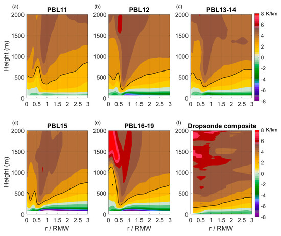
Figure 8.
Normalized radius-height plot of the azimuthally averaged vertical gradient of the virtual potential temperature (dθv/dz) over t = 84–108 h in the idealized HWRF simulations with (a) PBL11, (b) PBL12, (c) PBL13–14, (d) PBL15, and (e) PBL16–19 schemes. The dropsonde composite of dθv/dz is shown in (f). The black line is the 3K/km contour, which represents the thermodynamic PBL height. RMW is the radius of the maximum wind speed.
The azimuthally averaged temperature and humidity are compared as well between the simulations and observations in Figure 9 and Figure 10, respectively. All simulations show similar thermal structures between each other. In the surface layer, all simulations captured the observed trend for temperature to decrease with decreasing radius (except radially inward from the eyewall). Cione et al. [3] also showed a similar structure at 10 m altitude using extensive buoy observations. The magnitudes of simulated and observed temperature are comparable to each other near the surface (Figure 9). However, above the surface layer (>200 m), the air is much colder in all simulations than in the dropsonde composite. There is a 1 °C–3 °C cold bias in the HWRF simulations (Figure 9), which was also noted by Cione et al. [54] in their analysis of multiple HWRF cycles of Hurricane Maria (2017) using the 2017 operational configuration of the model.
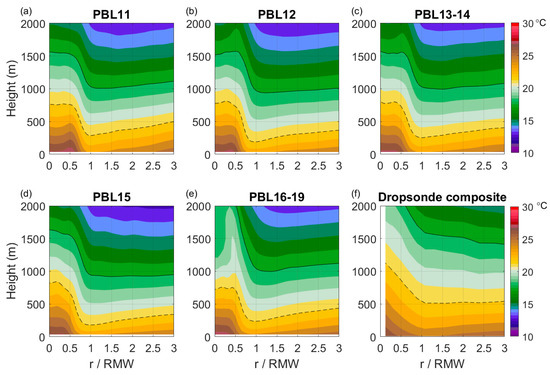
Figure 9.
Normalized radius-height plot of azimuthally averaged temperature (<T>) over t = 84–108 h in the idealized HWRF simulations with (a) PBL11, (b) PBL12, (c) PBL13–14, (d) PBL15, and (e) PBL16–19 schemes. The dropsonde composite of (<T>) is shown in (f). The black solid and dashed lines are the 18 °C and 22 °C contours, respectively. RMW is the radius of the maximum wind speed.
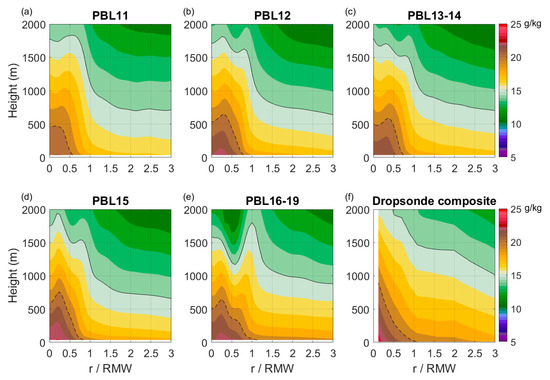
Figure 10.
Normalized radius-height plot of azimuthally averaged specific humidity (<q>) over t = 84–108 h in the idealized HWRF simulations with (a) PBL11, (b) PBL12, (c) PBL13–14, (d) PBL15, and (e) PBL16–19 schemes. The dropsonde composite of (<q>) is shown in (f). The black solid and dashed lines are the 15 g/kg and 20 g/kg contours, respectively. RMW is the radius of the maximum wind speed.
The moisture structure varies from simulation to simulation near the storm center in the surface layer (Figure 10). The surface layer is too dry in PBL11 and PBL13–14 compared to the observations, while it is close to the observations in PBL12, PBL15 and PBL16–19, except near the RMW, where it is still slightly dry. All simulations captured the increasing trend of specific humidity with decreasing radius throughout the PBL radially outward of the eyewall. Above the surface layer, there is a dry bias of 2–4 g kg−1 in all simulations compared to the observations.
The warm-core structure is compared among the simulations. Here the warm-core anomaly is calculated as the difference between the potential temperature averaged within a radius of 15 km from the storm center and that averaged within 200–300 km annulus (i.e., the environmental value), following Stern and Nolan [55]. Figure 11 shows the time evolution of the warm-core anomaly from all five simulations. Interestingly, double warm cores are present in the vertical in all simulations except PBL16–19, which only simulated the mid-level warm core.
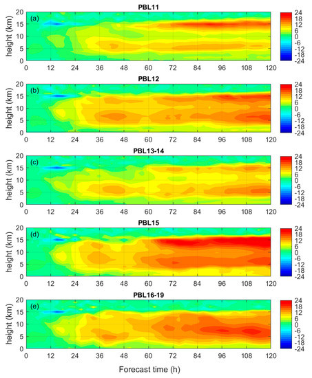
Figure 11.
Hovmöller diagram of the warm core anomaly (in K) in the idealized HWRF simulations with (a) PBL11, (b) PBL12, (c) PBL13–14, (d) PBL15, and (e) PBL16–19 schemes.
Both the timing of warm-core formation and the strength of the warm core, as indicated by the warm-core anomaly, vary from simulation to simulation for both the mid-level warm core and the upper-level warm core (when double warm cores are present). The warm core development in PBL11 and PBL13–14 is similar in that the lower warm core developed first at ~30 h lead time (t), and then the upper warm core developed. In PBL11, the upper warm core developed at t = 48 h, while the upper warm core developed at t = 60 h in PBL13–14. The difference in the warm core strength is also reflected in the stronger upper warm core in PBL11 relative to PBL13–14, while the lower warm core is stronger in PBL13–14. In both PBL12 and PBL15, warm cores tend to develop at t = 30 h; however, the double warm-core feature occurs much earlier in PBL12 than in PBL15. After t = 54 h, the strengths of both upper and lower warm cores are much larger in PBL15 than in PBL12. In PBL16–19, the low-level warm core with relatively strong anomaly developed at t = 36 at z = 5 km. A weak upper warm core attempts to develop in a short period of time (t = 28–36) but fails. The lower warm core moved upward to near z = 8 km after t = 60 h and maintained its strength after this time in PBL16–19.
Our results generally agree with Stern and Zhang [56] in that the perturbation temperature (i.e., warm-core anomaly) maximized at mid-levels during the RI period. After this period, our results show that the development of the double warm core varies with changes in the PBL schemes. Of note, the double warm core structure was also seen in HWRF real-case forecasts [57].
There is a strong correlation between the peak warm core anomaly and storm intensity in all simulations (Figure 12a). This is expected given that the warm-core anomaly is linked to hydrostatic balance [58]. Since the maximum storm intensity in PBL15 is the largest among all five experiments, the maximum warm core anomaly is also the largest.
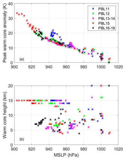
Figure 12.
Plots of (a) peak warm-core anomaly and (b) warm-core height as a function of the minimum sea level pressure (MSLP) in the idealized HWRF simulations with five different PBL schemes.
We define the warm-core height as the height of the maximum warm-core anomaly. The correlation between the warm-core height and the storm intensity is very weak in all simulations (Figure 12b). This result is consistent with that of Stern and Nolan [55] as well as Zhang et al. [39]. However, during the period of rapid intensification, when the MSLP falls from ~990 hPa at 18 h to ~960 hPa at 36 h (c.f., Figure 2b), the warm-core height generally descends and becomes located in the mid-levels (5–8 km) in almost all simulations (Figure 11). How the PBL physics is tied to warm-core development in TCs remains to be understood.
The impacts of HWRF PBL schemes on the distribution of deep convection (referred to as “convective bursts” hereafter) are evaluated next. A convective burst is defined by a grid point where the maximum vertical velocity in the vertical column is >3 m s−1 [32,59,60]. The count of convective bursts during the RI period (t = 12–30) is compared in Figure 13, which is stratified by the distance from the storm center normalized by the RMW at 2 km altitude. The total number of bursts inward from the RMW in PBL15 is the largest, while it is the smallest in PBL11. The total numbers of bursts inside the RMW of PBL12 and PBL16–19 are comparable to each other, when both runs have a comparable storm intensity and intensification rate (cf. Figure 2 and Figure 3). This result suggests that the total number of bursts is tied to storm intensity as well as intensification rate, with a faster intensifying and stronger storm associated with more bursts inside the RMW.
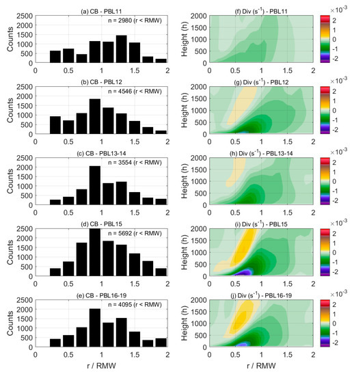
Figure 13.
(Left) Plots of counts of convective bursts (CB) as a function of radius normalized by the radius of maximum wind speed (RMW). The total number of bursts (n) inside the RMW is also shown. (Right) Normalized radius-height plots of the azimuthally averaged divergence (Div) during the rapid intensification period (12–30 h). These results are from idealized HWRF simulations with (a,f) PBL11, (b,g) PBL12, (c,h) PBL13–14, (d,i) PBL15, and (e,j) PBL16–19 schemes.
It is also evident from Figure 13 that the majority of the bursts are located at and inside the RMW (0.5–1 RMW) for PBL12, PBL13–14, PBL15, and PBL16–19, but the majority of the bursts are located outside the RMW (1–2 RMW) for PBL11. This result is consistent with previous observational and theoretical findings on the effect of deep convection on hurricane intensification from both the energy efficiency argument [61,62,63] and the angular momentum transfer point of view [64]. Zhang and Rogers [32] attributed the difference in the burst counts to the difference in the boundary layer inflow and convergence. Where the inflow is stronger, air parcels can advect radially closer to the storm center and the low-level convection can be initiated farther inward from the RMW. Our result in terms of the relationship of inflow strength (Figure 3), convergence (Figure 13f–j) and convective burst distribution (Figure 13a–e) supports the finding of Zhang and Rogers [32].
The structure of convection can also be evaluated using the contoured frequency by altitude diagrams (CFADs [65]) of vertical velocity (w). Previous studies have used CFADs of w to evaluate convective-scale structure in hurricane simulations relative to Doppler radar observations [50,66]. Here we also compare CFADs of w between the five idealized simulations in Figure 14, focusing on the eyewall region (r/RMW = 0.75–1.25) during the RI period (12–30 h).
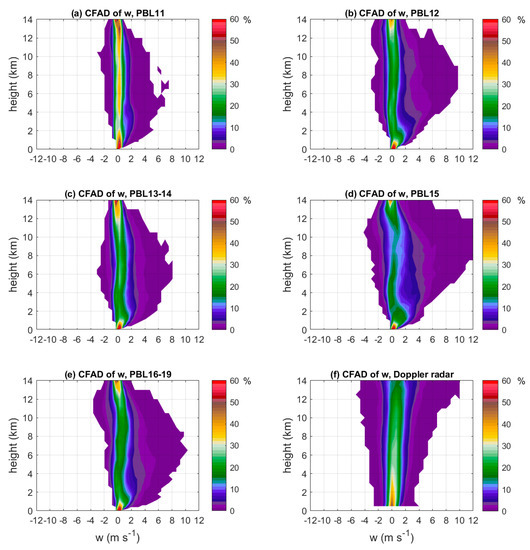
Figure 14.
Contoured Frequency by Altitude Diagrams (CFADs) of vertical velocity (w) in the eyewall region (0.75 < r/RMW < 1.25) during the rapid intensification period (12–30 h) in the idealized HWRF simulations with (a) PBL11, (b) PBL12, (c) PBL13–14, (d) PBL15, and (e) PBL16–19 schemes. CFAD of w from Doppler radar observations is shown in (f).
The strongest updrafts (i.e., the top 0.1–0.3% of the distributions of w > 5 m s−1) are more frequent in PBL12, PBL15, and PBL16–19 than in PBL11 and PBL13–14, especially above the boundary layer. The deep convection present in PBL12, PBL15, and PBL16–19 (c.f., Figure 13b,d,e) is therefore associated with stronger updrafts. Note that the boundary-layer convergence is tied to the forced updraft immediately above the PBL. For instance, the large convergence in PBL15 (Figure 13i) is consistent with the strong low-level (~2 km) peak updrafts seen in the CFADS of w (Figure 14d). Overall, the distribution of strong updrafts in PBL12, PBL15, and PBL16–19 is closer to Doppler radar observations (Figure 14f) than in PBL11 and PBL13–14.
The PBL mechanism related to radial advection of angular momentum (M) is the key component of the TC intensification theory of Smith et al. [6,67]. Unbalanced flow in the PBL is important for TC spin-up through the agradient force. Due to surface friction, gradient wind balance does not hold in the PBL, and the agradient forcing creates inflow. The agradient force (AF) per unit mass is defined as:
where ρ is the air density, p is the pressure, r is the radius, v is the tangential wind speed, and f is the Coriolis parameter. Figure 15b shows that the maximum azimuthally averaged AF (<AF>) is the largest in PBL15, while it is the smallest in PBL11 for almost all forecast lead times. During the RI period (t = 12–30 h), a sharp increase in <AF> is observed in all simulations (Figure 15b). The magnitude of the maximum <AF> is found to be positively correlated with the spin-up rate of the vortex (c.f., Figure 2). Our result also shows that the maximum <AF> is negatively correlated with the maximum <Km> (Figure 15a,b). The maximum convergence (Figure 15c) and maximum radial advection of the absolute angular momentum (-udM/dr, Figure 15d) in the PBL are also negatively correlated with the maximum <Km>. This result is consistent with the theory of Smith et al. [6] in that a faster intensifying TC is associated with the larger convergence of the absolute angular momentum in the PBL. Thus, our result demonstrates the important role of PBL physics in TC intensity change.
AF = −1/ρ dp/dr + v2/r + f v,
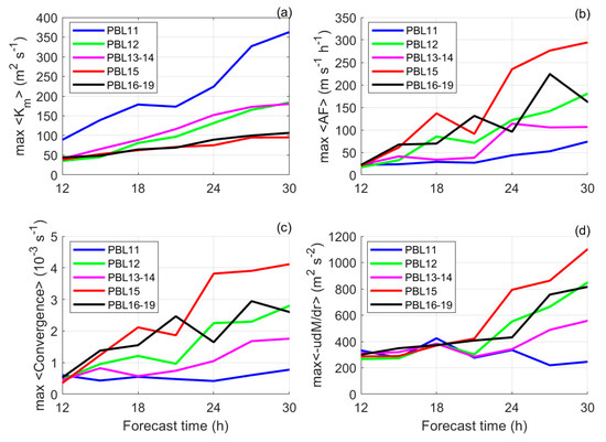
Figure 15.
Time series of (a) the maximum azimuthally averaged vertical eddy diffusivity (<Km>), (b) the maximum azimuthally averaged agradient force per unit mass (<AF>), (c) the maximum azimuthally averaged convergence in the PBL, and (d) the maximum azimuthally averaged radial advection of absolute angular momentum (-udM/dr) in the idealized HWRF simulations with 5 different PBL schemes during the rapid intensification period (t = 12–30 h).
4. Discussion and Conclusions
This study reviews the PBL schemes that have been used in the operational HWRF model. The effects of these PBL schemes on TC intensification and structure are evaluated using idealized HWRF simulations. Our results show that the weakest storm is in the simulation with the original GFS PBL scheme in the 2011 and prior versions of HWRF, while the simulated storm is the strongest using the PBL scheme in the 2015 version of HWRF (PBL15), in which the wind-speed dependent parameterization of vertical eddy diffusivity was added. The simulation with the PBL scheme in the 2016–2019 version of HWRF (PBL16–19) that includes a mass-flux approach also produces a strong storm, but it is slightly weaker than the simulated storm in PBL15. It is also found that both the intensification rate during the RI (or spin-up) period and the maximum storm intensity of the five-day simulations vary with the PBL schemes. Our result suggests that the vertical eddy diffusivity is an important parameter that influences TC intensity and intensification rate, in that the smaller the Km value in the PBL, the faster a simulated storm tends to intensify and the stronger the storm ultimately becomes.
Simulated TC structures are also modulated by the PBL schemes. For instance, the strength of the inflow, the location and strength of the tangential wind maximum, PBL convergence, and the inflow layer depth all vary in these simulations. The structural differences help explain the differences in simulated storm intensity. When the vertical turbulent mixing is small in the PBL scheme, the simulated TC inflow is strong and low-level convergence is large. Stronger inflow that is associated with larger agradient force advects more absolute angular momentum towards the storm center so that the vortex deepens faster in the PBL, which is consistent with the TC spin-up theory. Larger convergence triggers stronger convection within and immediately above the boundary layer. These strong updrafts act to ventilate air from the PBL, vertically advecting absolute angular momentum above the PBL and favoring TC intensification [6,32,39].
Our result also shows that the distribution of deep convection differs between the simulations with different PBL schemes, in terms of both the total number and radial location of convective bursts. More convective bursts located inside the low-level RMW are seen in simulations with PBL schemes that have smaller Km such as PBL15 and PBL16–19. This difference in deep convection distribution would lead to differences in the diabatic heating [67]. According to previous theoretical and observational studies [61,62,63,64], when the deep convection and strong diabatic heating are located inside the RMW, storms tend to intensify more rapidly. Our result agrees with these studies.
The warm-core structure also varies in simulations with different PBL schemes, particularly in the timing of warm core formation, the number of warm cores, and the height and strength of the warm core anomaly. All simulations, except the one with the PBL16–19, exhibited a double warm core structure. Since the PBL16–19 version scheme is an EDMF-type scheme that contains both eddy diffusivity and mass flux components, while the rest of the schemes only contain an eddy diffusivity component, our results suggest that the addition of the mass-flux scheme alters the upper-level thermal structure. Future studies will evaluate how and why the PBL processes are linked to the warm core development in real-case simulations and observations. Notably, our results suggest that the effect of the mass-flux component of the EDMF scheme on TC intensity and kinematic structure may be small as long as Km is well parameterized in the scheme.
Compared to the dropsonde and Doppler radar observations, improvements in kinematic structure were obtained in simulations with recent PBL schemes (i.e., PBL15, PBL16–19). PBL16–19 performed best among the five PBL schemes. However, the simulated upper PBL is much cooler and drier than observations in all simulations. These dry and cool biases were also found in a previous case study that compared a HWRF forecast with unmanned aircraft observations [54]. The biases may be tied to the configuration of turbulent mixing of thermal properties in the PBL schemes, especially the entrainment parameterization near the top of the PBL. Thus, it is recommended that future development of the PBL scheme should focus on improving the representation of the thermodynamic structure in HWRF. Parameterizations of enthalpy fluxes and entrainment process in the PBL should be examined against observations or large eddy simulations to reduce the biases in temperature and humidity in those simulations. We note that the comparisons of idealized simulations with observational composites were conducted in a climatological sense in the present study. Future studies will further evaluate the structural differences between operational forecasts and observations of real TCs and improve model physics to reduce the biases in the modeled structures.
Author Contributions
Conceptualization, J.A.Z., E.A.K., and R.F.R.; methodology, J.A.Z., E.A.K., M.K.B., R.F.R., F.D.M. and P.Z.; software, J.A.Z and E.A.K.; validation, J.A.Z., E.A.K., F.D.M., R.F.R., and P.Z.; formal analysis, J.A.Z.; resources, F.D.M., E.A.K., and M.K.B.; data curation, E.A.K. and M.K.B.; writing—original draft preparation, J.A.Z. and E.A.K.; writing—review and editing, M.K.B., R.F.R., F.D.M., and P.Z.; visualization, J.A.Z., E.A.K., and M.K.B.; supervision, F.D.M.; project administration, F.D.M. and M.K.B.; funding acquisition, J.A.Z., E.A.K., and P.Z. All authors have read and agreed to the published version of the manuscript.
Funding
This research was funded by National Oceanic and Atmospheric Administration (NOAA) Grants NA14NWS4680028, NA16NWS4680029, NA14NWS4680030, and NA17OAR4320101; National Science Foundation (NSF) Grants AGS1822128 and AGS1822238; and Office of Naval Research (ONR) Grant N00014-20-1-2071. J.A.Z. also acknowledges the support from the Developmental Testbed Center (DTC) visitor program. The DTC is funded by NOAA, the U.S. Air Force, the National Center for Atmospheric Research (NCAR), and NSF.
Acknowledgments
The authors would like to acknowledge scientists and model developers who have contributed to HWRF documentation, maintenance and upgrades. The authors are also grateful to scientists and flight crew who have participated the hurricane field program and helped collect the observations used in this study.
Conflicts of Interest
The authors declare no conflict of interest.
References
- Emanuel, K.A. An Air-Sea Interaction Theory for Tropical Cyclones. Part I: Steady-State Maintenance. J. Atmos. Sci. 1986, 43, 585–605. [Google Scholar] [CrossRef]
- Riemer, M.; Montgomery, M.T.; Nicholls, M.E. A new paradigm for intensity modification of tropical cyclones: Thermodynamic impact of vertical wind shear on the inflow layer. Atmos. Chem. Phys. 2010, 10, 3163–3188. [Google Scholar] [CrossRef]
- Cione, J.J.; Kalina, E.A.; Zhang, J.A.; Uhlhorn, E.W. Observations of Air–Sea Interaction and Intensity Change in Hurricanes. Mon. Weather Rev. 2013, 141, 2368–2382. [Google Scholar] [CrossRef]
- Montgomery, M.; Smith, R. Paradigms for tropical cyclone intensification. J. South. Hemisph. Earth Syst. Sci. 2014, 64, 37–66. [Google Scholar] [CrossRef]
- Montgomery, M.T.; Zhang, J.A.; Smith, R.K. An analysis of the observed low-level structure of rapidly intensifying and mature hurricane Earl (2010). Q. J. R. Meteorol. Soc. 2014, 140, 2132–2146. [Google Scholar] [CrossRef]
- Smith, R.K.; Montgomery, M.T.; Van Sang, N. Tropical cyclone spin-up revisited. Q. J. R. Meteorol. Soc. 2009, 135, 1321–1335. [Google Scholar] [CrossRef]
- Smith, R.K.; Zhang, J.A.; Montgomery, M.T. The dynamics of intensification in a Hurricane Weather and Research Forecast of Hurricane Earl (2010). Q. J. R. Meteorol. Soc. 2017, 143, 297–308. [Google Scholar] [CrossRef]
- Zhang, J.A.; Cione, J.J.; Kalina, E.A.; Uhlhorn, E.W.; Hock, T.; Smith, J.A. Observations of Infrared sea surface temperature and air-sea interaction in Hurricane Edouard (2014) using GPS dropsondes. J. Atmos. Ocean. Technol. 2017, 34, 1333–1349. [Google Scholar] [CrossRef]
- Nguyen, L.T.; Rogers, R.; Zawislak, J.; Zhang, J.A. Assessing the Influence of Convective Downdrafts and Surface Enthalpy Fluxes on Tropical Cyclone Intensity Change in Moderate Vertical Wind Shear. Mon. Weather Rev. 2019, 147, 3519–3534. [Google Scholar] [CrossRef]
- Ahern, K.; Bourassa, M.A.; Hart, R.E.; Zhang, J.A.; Rogers, R.F. Observed Kinematic and Thermodynamic Structure in the Hurricane Boundary Layer during Intensity Change. Mon. Weather. Rev. 2019, 147, 2765–2785. [Google Scholar] [CrossRef]
- Chen, X.; Zhang, J.A.; Marks, F.D. A thermodynamic pathway leading to rapid intensification of tropical cyclones in shear. Geophys. Res. Lett. 2019, 46, 9241–9251. [Google Scholar] [CrossRef]
- Bryan, G.H.; Worsnop, R.P.; Lundquist, J.K.; Zhang, J.A. A simple method for simulating wind profiles in the boundary layer of tropical cyclones. Bound. Layer Meteor. 2017, 162, 475–502. [Google Scholar] [CrossRef]
- Worsnop, R.P.; Bryan, G.H.; Lundquist, J.K.; Zhang, J.A. Using Large-Eddy Simulations to define spectral and coherence characteristics of the hurricane boundary layer for wind-energy applications. Boundary Layer Meteor. 2017, 165, 55–86. [Google Scholar] [CrossRef]
- Worsnop, R.P.; Lundquist, J.K.; Bryan, G.H.; Damiani, R.; Musial, W. Gusts and shear within hurricane eyewalls can exceed offshore wind turbine design standards. Geophys. Res. Lett. 2017, 44, 6413–6420. [Google Scholar] [CrossRef]
- Donelan, M.A.; Haus, B.K.; Reul, N.; Plant, W.J.; Stiassnie, M.; Graber, H.C.; Brown, O.B.; Saltzman, E.S. On the limiting aerodynamic roughness of the ocean in very strong winds. Geophys. Res. Lett. 2014, 31, L18306. [Google Scholar] [CrossRef]
- Bell, M.M.; Montgomery, M.T.; Emanuel, K.A. Air–sea enthalpy and momentum exchange at major hurricane wind speeds observed during CBLAST. J. Atmos. Sci. 2012, 69, 3197–3222. [Google Scholar] [CrossRef]
- Braun, S.A.; Tao, W.K. Sensitivity of High-Resolution Simulations of Hurricane Bob (1991) to Planetary Boundary Layer Parameterizations. Mon. Weather. Rev. 2000, 128, 3941–3961. [Google Scholar] [CrossRef]
- Smith, R.K.; Thomsen, G.L. Dependence of tropical-cyclone intensification on the boundary-layer representation in a numerical model. Q. J. R. Meteorol. Soc. 2010, 136, 1671–1685. [Google Scholar] [CrossRef]
- Nolan, D.S.; Zhang, J.A.; Stern, D.P. Evaluation of planetary boundary layer parameterizations in tropical cyclones by comparison of in situ data and high-resolution simulations of Hurricane Isabel (2003). Part I: Initialization, maximum winds, and outer-core boundary layer structure. Mon. Weather Rev. 2009, 137, 3651–3674. [Google Scholar] [CrossRef]
- Zhu, P.; Menelaou, K.; Zhu, Z. Impact of subgrid-scale vertical turbulent mixing on eyewall asymmetric structures and mesovortices of hurricanes. Quart. J. Roy. Meteor. Soc. 2013, 140, 416–438. [Google Scholar] [CrossRef]
- Ming, J.; Zhang, J.A. Effects of surface flux parameterization on numerically simulated intensity and structure of Typhoon Morakot (2009). Advances Atmos. Sci. 2016, 33, 58–72. [Google Scholar] [CrossRef]
- Bryan, G.H. Effects of surface exchange coefficients and turbulence length scales on the intensity and structure of numerically simulated hurricanes. Mon. Wea. Rev. 2012, 140, 1125–1143. [Google Scholar] [CrossRef]
- Kilroy, G.; Smith, R.K.; Montgomery, M.T. Why do model tropical cyclones grow progressively in size and decay in intensity after reaching maturity? J. Atmos. Sci. 2016, 73, 487–503. [Google Scholar] [CrossRef]
- Kepert, J.D. Choosing a Boundary Layer Parameterization for Tropical Cyclone Modeling. Mon. Weather Rev. 2012, 140, 1427–1445. [Google Scholar] [CrossRef]
- Gall, R.; Franklin, J.; Marks, F.; Rappaport, E.N.; Toepfer, F. The Hurricane Forecast Improvement Project. Bull. Amer. Meteor. Soc. 2013, 94, 329–343. [Google Scholar] [CrossRef]
- Gopalakrishnan, S.G.; Marks, F., Jr.; Zhang, J.A.; Zhang, X.; Bao, J.W.; Tallapragada, V. A study of the impacts of vertical diffusion on the structure and intensity of the tropical cyclones using the high-resolution HWRF system. J. Atmos. Sci. 2013, 70, 524–541. [Google Scholar] [CrossRef]
- Zhang, J.A.; Marks, F.D. Effects of horizontal eddy diffusivity on tropical cyclone intensity change and structure in idealized three-dimensional numerical simulations. Mon. Wea. Rev. 2015, 143, 3981–3995. [Google Scholar] [CrossRef]
- Bu, Y.P.; Fovell, R.G.; Corbosiero, K.L. The influences of boundary layer vertical mixing and cloud-radiative forcing on tropical cyclone size. J. Atmos. Sci. 2017, 74, 1273–1292. [Google Scholar] [CrossRef]
- Kieu, C.Q.; Tallapragada, V.; Hogsett, W. On the onset of the tropical cyclone rapid intensification in the HWRF model. Geophys. Res. Lett. 2014, 9, 3298–3306. [Google Scholar] [CrossRef]
- Tyner, B.; Zhu, P.; Zhang, J.A.; Gopalakrishnan, S.; Marks, F.M.; Tallapragada, V. A top-down pathway to secondary eyewall formation in simulated tropical cyclones. J. Geophys. Res. Atmos. 2017, 123, 174–197. [Google Scholar] [CrossRef]
- Leighton, H.; Gopalakrishnan, S.; Zhang, J.A.; Rogers, R.F.; Zhang, Z.; Tallapragada, V. Azimuthal distribution of deep convection, environmental factors and tropical cyclone rapid intensification: A perspective from HWRF ensemble forecasts of Hurricane Edouard (2014). J. Atmos. Sci. 2018, 75, 275–295. [Google Scholar] [CrossRef]
- Zhang, J.A.; Rogers, R.F. Effects of Parameterized Boundary Layer Structure on Hurricane Rapid Intensification in Shear. Mon. Weather Rev. 2019, 147, 853–871. [Google Scholar] [CrossRef]
- Biswas, M.K.; Zhang, J.A.; Grell, E.; Kalina, E.; Newman, K.; Bernardet, L.; Carson, L.; Frimel, J.; Grell, G. Evaluation of the Grell-Freitas convective scheme in the Hurricane Weather Research and Forecasting (HWRF) model. Weather Forecast. 2020, 35, 1017–1033. [Google Scholar] [CrossRef]
- Zhu, P.; Tyner, B.; Zhang, J.A.; Aligo, E.; Gopalakrishnan, S.; Marks, F.D.; Mehra, A.; Tallapragada, V. Role of eyewall and rainband eddy forcing in tropical cyclone intensification. Atmos. Chem. Phys. 2019, 19, 14289–14310. [Google Scholar] [CrossRef]
- Troen, I.B.; Mahrt, L. A simple model of the atmospheric boundary layer; sensitivity to surface evaporation. Bound. Layer Meteorol. 1986, 37, 129–148. [Google Scholar] [CrossRef]
- Han, J.; Pan, H.-L. Revision of convection and vertical diffusion schemes in the ncep global forecast system. Weather Forcasting 2011, 26, 520–533. [Google Scholar] [CrossRef]
- Zhang, J.A.; Gopalakrishnan, S.; Marks, F.D.; Rogers, R.F.; Tallapragada, V. A developmental framework for improving hurricane model physical parameterization using aircraft observations. Trop. Cyclone Res. Rev. 2012, 1, 419–429. [Google Scholar]
- Tallapragada, V.; Kieu, C.; Kwon, Y.; Trahan, S.; Liu, Q.; Zhang, Z.; Kwon, I. Evaluation of storm structure from the operational HWRF during 2012 implementation. Mon. Wea. Rev. 2014, 142, 4308–4325. [Google Scholar] [CrossRef]
- Zhang, J.A.; Nolan, D.S.; Rogers, R.F.; Tallapragada, V. Evaluating the Impact of Improvements in the Boundary Layer Parameterization on Hurricane Intensity and Structure Forecasts in HWRF. Mon. Wea. Rev. 2015, 143, 3136–3155. [Google Scholar] [CrossRef]
- Bu, Y.P.; Fovell, R.G.; Corbosiero, K.L. Influence of cloud-radiative forcing on tropical cyclone structure. J. Atmos. Sci. 2014, 71, 1644–1662. [Google Scholar] [CrossRef]
- Han, J.; Witek, M.L.; Teixeira, J.; Sun, R.; Pan, H.; Fletcher, J.K.; Bretherton, C.S. Implementation in the ncep gfs of a hybrid eddy-diffusivity mass-flux (EDMF) boundary layer parameterization with dissipative heating and modified stable boundary layer mixing. Weather Forcasting 2016, 31, 341–352. [Google Scholar] [CrossRef]
- Wang, W.; Sippel, J.A.; Abarca, S.; Zhu, L.; Liu, B.; Zhang, Z.; Mehra, A.; Tallapragada, V. Improving ncep hwrf simulations of surface wind and inflow angle in the eyewall area. Weather Forecasting 2018, 33, 887–898. [Google Scholar] [CrossRef]
- Biswas, M.K. Hurricane Weather Research and Forecasting (HWRF) Model: 2017 Scientific Documentation. NCAR Technical Notes, NCAR/TN-544+STR. 2018. Available online: https://opensky.ucar.edu/islandora/object/technotes:563 (accessed on 4 October 2020).
- Gray, W.; Ruprecht, E.; Phelps, R. Relative humidity in tropical weather systems. Mon. Weather Rev. 1975, 103, 685–690. [Google Scholar] [CrossRef]
- Wang, Y. An inverse balance equation in sigma coordinates for model initialization. Mon. Weather Rev. 1995, 123, 482–488. [Google Scholar] [CrossRef][Green Version]
- Aligo, E.; Ferrier, B.; Thompson, G.; Carley, J.R.; Rogers, E.; Dimego, J. The New-Ferrier-Aligo Microphysics in the NCEP 3-km NAM Nest. In Proceedings of the 97th AMS Annual Meeting, Seattle, WA, USA, 21–26 January 2017. [Google Scholar]
- Grell, G.A.; Freitas, S.R. A scale and aerosol aware stochastic convective parameterization for weather and air quality modeling. Atmos. Chem. Phys. 2014, 14, 5233–5250. [Google Scholar] [CrossRef]
- Iacono, M.J.; Delamere, J.S.; Mlawer, E.J.; Shephard, M.W.; Clough, S.A.; Collins, W.D. Radiative forcing by long-lived greenhouse gases: Calculations with the AER radiative transfer models. J. Geophys. Res. 2008, 113, D13103. [Google Scholar] [CrossRef]
- Edson, J.B. Coauthors On the exchange of momentum over the open ocean. J. Phys. Oceanogr. 2013, 43, 1589–1610. [Google Scholar] [CrossRef]
- Zhang, J.A.; Rogers, R.F.; Nolan, D.S.; Marks, F.D., Jr. On the Characteristic Height Scales of the Hurricane Boundary Layer. Mon. Weather Rev. 2011, 139, 2523–2535. [Google Scholar] [CrossRef]
- Nolan, D.S.; Atlas, R.A.; Bhatia, K.T.; Bucci, L.R. Development and validation of a hurricane nature run using the joint OSSE nature run and the WRF model. J. Adv. Model. Earth Sys. 2013, 5, 382–405. [Google Scholar] [CrossRef]
- Kepert, J.D.; Schwendike, J.; Ramsay, H. Why is the tropical cyclone boundary layer not “well mixed”? J. Atmos. Sci. 2016, 73, 957–973. [Google Scholar] [CrossRef]
- Gao, K.; Ginis, I. On the generation of roll vortices due the inflection point instability of the hurricane boundary layer flow. J. Atmos. Sci. 2014, 71, 4292–4307. [Google Scholar] [CrossRef]
- Cione, J.J.; Bryan, G.H.; Dobosy, R.; Zhang, J.A.; de Boer, G.; Aksoy, A.; Wadler, J.B.; Kalina, E.A.; Dahl, B.A.; Neuhaus, K.R.J.; et al. Eye of the storm: Observing hurricanes with a small unmanned aircraft system. Bull. Am. Meteor. Soc. 2020, 101, E186–E205. [Google Scholar] [CrossRef]
- Stern, D.P.; Nolan, D.S. On the Height of the Warm Core in Tropical Cyclones. J. Atmos. Sci. 2012, 69, 1657–1680. [Google Scholar] [CrossRef]
- Stern, D.P.; Zhang, F. How Does the Eye Warm? Part I: A Potential Temperature Budget Analysis of an Idealized Tropical Cyclone. J. Atmos. Sci. 2013, 70, 73–90. [Google Scholar] [CrossRef]
- Kieu, C.Q.; Tallapragada, V.; Zhang, D.; Moon, Z. On the Development of Double Warm-Core Structures in Intense Tropical Cyclones. J. Atmos. Sci. 2016, 73, 4487–4506. [Google Scholar] [CrossRef]
- Zhang, D.-L.; Chen, H. Importance of the upper-level warm core in the rapid intensification of a tropical cyclone. Geophys. Res. Lett. 2012, 39. [Google Scholar] [CrossRef]
- Chen, H.; Gopalakrishnan, S. A study on the asymmetric rapid intensification of Hurricane Earl (2010) using the HWRF system. J. Atmos. Sci. 2015, 72, 531–550. [Google Scholar] [CrossRef]
- Rogers, R.F. Convective-scale structure and evolution during a high-resolution simulation of tropical cyclone rapid intensification. J. Atmos. Sci. 2010, 67, 44–70. [Google Scholar] [CrossRef]
- Schubert, W.H.; Hack, J.J. Inertial stability and tropical cyclone development. J. Atmos. Sci. 1982, 39, 1687–1697. [Google Scholar] [CrossRef]
- Nolan, D.S.; Moon, Y.; Stern, D.P. Tropical cyclone intensification from asymmetric convection: Energetics and efficiency. J. Atmos. Sci. 2007, 64, 3377–3405. [Google Scholar] [CrossRef]
- Rogers, R.F.; Reasor, P.; Lorsolo, S. Airborne Doppler observations of the inner-core structural differences between intensifying and steady-state tropical cyclones. Mon. Weather Rev. 2013, 141, 2970–2991. [Google Scholar] [CrossRef]
- Smith, R.K.; Montgomery, M.T. The efficiency of diabatic heating and tropical cyclone intensification. Quart. J. Roy. Meteor. Soc. 2016, 142, 2081–2086. [Google Scholar] [CrossRef]
- Yuter, S.E.; Houze, R.A., Jr. Three-dimensional kinematic and microphysical evolution of Florida cumulonimbus. Part III: Vertical mass transport, mass divergence, and synthesis. Mon. Weather Rev. 1995, 123, 1964–1983. [Google Scholar] [CrossRef]
- Rogers, R.F.; Black, M.L.; Chen, S.S.; Black, R.A. An evaluation of microphysics fields from mesoscale model simulations of tropical cyclones, Part I: Comparisons with observations. J. Atmos. Sci. 2007, 64, 1811–1834. [Google Scholar] [CrossRef]
- Zhang, J.A.; Rogers, R.F.; Tallapragada, V. Impact of parameterized boundary layer structure on tropical cyclone rapid intensification forecasts in HWRF. Mon. Weather Rev. 2017, 145, 1413–1426. [Google Scholar] [CrossRef]


© 2020 by the authors. Licensee MDPI, Basel, Switzerland. This article is an open access article distributed under the terms and conditions of the Creative Commons Attribution (CC BY) license (http://creativecommons.org/licenses/by/4.0/).