Abstract
The seasonal and diurnal variability of the wind resource in Northern Mexico is examined. Fourteen weather stations were grouped according to the terrain morphology and weather systems that affect the region to evaluate the impact on wind ramps and high wind persistent events. Four areas driven by weather systems seasonality are identified. Wind power ramps and persistent generation events are produced by cold fronts in winter, while mesoscale convective systems and local circulations are dominant in summer. Moreover, the 2013 wind forecast of the Rapid Refresh Model (RAP) and the North American Mesoscale Forecast System (NAM) forecast systems were also assessed. In general, both systems have less ability to predict mesoscale events and local circulations over complex topography, underestimating strong winds and overestimating weak winds. Wind forecast variations in the mesoscale range are smoother than observations due to the effects of spatial and temporal averaging, producing fewer wind power ramps and longer lasting generation events. The study carried out shows the importance of evaluating operational models in terms of wind variability, wind power ramps and persistence events to improve the regional wind forecast. The characteristics of weather systems and topography of Mexico requires model refinements for proper management of the wind resource.
1. Introduction
Wind energy has undergone rapid growth in recent years, with record numbers of new worldwide wind power operative plants every year. The expansion of wind energy using existing technologies, power system improvements and creative policy making is leading the world towards a reduction on dependence of non-renewable energy sources. Mexico generates 71.2% of electricity from fossil fuels. The wind power installed capacity in Mexico is 4875 MW, approximately 20% of installed capacity of renewable energies [1].
The main drawback of wind power is the intermittent generation related to wind speed variability. Electricity generated by wind turbines can be highly variable at multi-time scales that range from sub-hourly to seasonal. Wind power needs to be scheduled to balance power generation and load demand in power systems. Large penetration of wind power could have a large impact on the operation and security of electric power grids [2].
Wind power ramps (sudden and large changes in wind energy generation) produce fluctuations of wind energy that can be challenging for system operators [3]. Mismanagement of ramps occurrence can reduce the power generation of a wind farm, causing differences between the real and estimated generation cost. An adequate assessment of potential wind power should include the characterization of wind power ramps.
Despite their importance for the operations of wind farms, there is no standard definition of wind power ramps. Instead, multiple wind ramp definitions exist. These definitions consider ramp characteristics such as their magnitude and duration [4]. The magnitude threshold of a ramp is usually expressed as a percentage of the rated power [4,5,6,7,8]. Usually, multiple ramp definitions may be required to be operational simultaneously as the appropriate threshold depends on the users. This leads to measuring the skill of numerical weather prediction models under different ramp definitions, from binary (ramp/non-ramp) [8], which can be very sensitive to threshold values [9], to more sophisticated ones [10,11]. Sensitivity studies of wind speed forecast during wind ramp events to parameters such as initial condition, model resolution and type of event has been done in order to explore forecast uncertainty [12].
The understanding of the weather systems’ (WS) role and better anticipation of ramp events could help to achieve an efficient integration of wind energy in power systems. One of the keys to successfully managing wind energy is the ability to accurately forecast the expected amount of wind energy supplied to the power grid. Approaches to wind power forecasting have improved in recent years with an emphasis on short-term wind forecasting (18–24 h) [13,14,15]. The improvements have been achieved by new physics parameterization methods, and enhanced data assimilation techniques coupled to better-quality data available for assimilation [16].
Integration and management of wind power ramps have been topics of interest in places with significant wind power penetration [17,18,19,20], however, there are no studies about wind ramps variability associated with wind power generation in Mexico. The understanding of WS that causes ramp events is an important precursor to the development of a successful ramp forecast procedure [4].
Several studies have found that wind ramps occurrence at mid-latitudes is caused by extratropical cyclones in the winter season [5,19,21]. During summer, wind ramps are related to mesoscale systems: boundary layer processes, mountain-valley breezes, sea-land breezes and mesoscale convective systems (MCS) that produce changes of short duration in the wind speed [13,14].
Mexico is frequently affected by winter cold surges that propagate from the mid-latitudes, as a form of atmospheric mid-latitude-tropical interactions [22]. Meanwhile, during summer the mesoscale events are the main modulators of the tropical circulation. Furthermore, the Mexican topography is complex, with topographic gradients that can go from 5700 m to sea level in less than 100 km [23].
Some numerical weather prediction studies at multiple time horizons have shown that the ability of the Weather Research and Forecasting Model (WRF) to accurately forecast wind speed and ramp events mainly depends on the topography, the initial conditions, the spatial resolution and the parameterization scheme in the boundary layer [13,24,25,26]. The accuracy of the forecast is also related to domain sizes, the number and spacing of the vertical levels, and other parameterizations such as land surface. Carvalho et al. [24] showed that wind forecasts over the Iberian Peninsula with 90 km, 18 km and 3.6 km horizontal grid spacing are more accurate in regions with flat topography and the ability decreases in complex topography. In these sites, the thermal circulations and the flows induced by the terrain characteristics are crucial for the prediction of wind speed and direction.
This study examines the role of WS in wind power ramps and wind variability in Northern Mexico. Due to the variety of WS that affect the region, it is important to understand the factors that affect wind ramps, high and low generation events. To address this issue, seasonal and diurnal variations in wind energy are analyzed. Furthermore, proper management of wind farms involves also wind forecast. Therefore, a short-term wind forecast verification is carried out for two operational systems, namely the North American Mesoscale Forecast System (NAM) [27] and the Rapid Refresh Model (RAP) [15], which cover Northern Mexico. The purpose of this exercise is to examine the performance of these models against observations at weather stations which experience the influence of different WS. Ramp forecasting skill is assessed by using ramp indices considering the timing and magnitude of wind power changes.
The rest of the paper is organized as follows. Section 2 describes the data and methodology used, including a brief description of the operational NAM [27] and RAP [15] models. Section 3 examines the wind variability for 14 weather stations and the wind forecast skill of NAM and RAP models for 2013. An evaluation of models to predict wind power ramp and extreme events is also discussed. Issues such as intermittency, variability and uncertainty in the forecasted wind power output are discussed. The conclusions are presented in Section 4.
2. Data and Method
2.1. Weather Stations
Wind variability in Northern Mexico is examined using 14 weather stations of the Mexico National Meteorological Service, the 10 m wind speed and direction are measured with a frequency of 10 min. The raw time series showed discontinuities and inconsistencies (e.g., persistent direction for several days, unrealistic winds, discrepancies on wind speed units). Therefore, a quality control process was performed on the raw data. During quality control, records with wind speed or wind direction beyond plausible values were filtered out as were periods with constant wind speed or wind direction or abrupt changes in the wind speed values. The former are typical of instrument fails and the latter correspond to changes in wind speed units, for example, m/s to kt. Wind speed and wind direction were also compared to wind gust speed and direction for internal consistency. This procedure resulted in some stations with nine years and others with only four years of consistent data (Table 1). The analysis was performed using the hourly average wind.

Table 1.
Classification of the sites by topography and weather systems.
The fraction of hours that the surface winds exceeded 3 m/s, which corresponds to the cut-in wind speed in a typical power curve, was calculated. This metric is proportional to wind farm operation hours. However, it does not show the amount of power generated [28,29].
The exceedance frequency threshold of the 3 m/s for all stations has a terrain dependence on near-surface wind speed (Figure 1), and suggests different weather systems modulating the wind on the regions. Wind speed days means the number of hours >3 m/s divided by 24. Areas exceeding the wind threshold for 226 to 250 days per year are located in the Baja California Coast, where some wind farms are operating (Figure S1, in supplementary material). In contrast, in-land regions exceed this threshold just around 175 days at the Mexican Plateau. Low-frequency modes, such as El Niño-Southern Oscillation (ENSO), Pacific Decadal Oscillation (PDO), and Atlantic Multidecadal Oscillation (AMO), might influence the occurrence of extreme winds [30]. However, this influence is not captured by the short-time data sample under analysis here.

Figure 1.
(A) Study area and (B) domain of the North American Mesoscale Forecast System (NAM) (red line) and the Rapid Refresh Model (RAP) (blue line) mesoscale models. Shaded areas represent terrain height (m) with slopes greater than 5°. The size of the circle indicates wind speed days >3 m/s. The color in the circles indicate the regions: the Baja California Peninsula in red, Gulf of California in green, Plateau in blue and Northeastern Mexico in yellow. Topographic slopes were calculated as the magnitude of the gradient for the GTOPO30 [32] digital elevation model with a horizontal grid spacing of 30 arc seconds (~1 km).
Complex topography is a term commonly used in wind power assessment studies, but an objective definition is not given. In this study, the topography complexity classes are defined as in Bingoel [31], but with the incorporation of a 50 km radius of influence (Table 1). Complex topography is considered when terrain slope exceeds 10° within the radius of influence, moderately complex when the maximum slope value is between 5° and 10°, and flat for slopes of less than 5°. The reason for including a radius of influence is that boundary layer winds are modified by the surrounding topography of the site of interest. Storm downdrafts, local circulations such as sea-land breeze and mountain-valley breeze develop due to horizontal gradients of temperature, which are caused or reinforced by the terrain slopes.
2.2. Forecast Models
NOAA’s Rapid Refresh (RAP) [7] and North American Mesoscale Forecast System (NAM) [27] models were selected as the basis for the wind forecast assessment over Northern Mexico. The reasons for choosing the regional models were that both models’ domains cover Northern Mexico (see the model domain in Figure 1b), the output from both is freely provided by NCEP at hourly resolution, and both models utilize the underlying Advanced Research version of the WRF Model [33], which has been widely used by the scientific community for wind forecasting [13,14].
The RAP analysis and forecast system provides hourly forecasts over North America with a 13 km grid spacing for up to 18 h, with a new data assimilation forecast cycle using latest hourly observations to run new forecasts every hour [15]. The RAP uses sigma coordinates with 51 vertical layers with a high vertical resolution near surface. RAP uses a community supported data assimilation package, the Gridpoint Statistical Interpolation, to carry out 3-dimensional hybrid ensemble/variational data assimilation [34]. Among their applications are transportation system management, severe weather, and energy.
The NAM [27] run by the National Centers for Environmental Prediction (NCEP) is initialized hourly with a 12 h data assimilation cycle, producing 3 hourly analysis updates using the regional Gridpoint Statistical Interpolation hybrid ensemble analysis. NAM forecast up to 84 h with 12 km horizontal resolution and 60 vertical levels with hybrid sigma-pressure coordinates.
2.3. Method
2.3.1. Weather Station Groups
The 14 stations were grouped according to the terrain morphology and the WS affecting the area during the dry and wet seasons (Table 1). In Mexico, the winter rainfall pattern is dominated by mid-latitude WS [35,36] and in the summer by easterly tropical waves and tropical cyclones. These are important moisture carriers responsible for the seasonal precipitation (May–November) over the Mesoamerica [37].
Seasonal and daily wind roses were constructed to examine the WS that modulate the wind at each station. Prevailing intense winds from persistent direction during winter (e.g., CDCU) suggest passage of frontal systems. Examination of front position with the horizontal gradient of equivalent potential temperature at 700 and 500 mb and the horizontal surface wind (not shown) was calculated using ERA5 [38] reanalysis data. The analysis showed prefrontal and postfrontal wind intensification at weather stations. Cold front reports in newspapers and from the monthly climate review of CONAGUA (National Water Commission of Mexico) from 2014–2015 over Northern Mexico were also consulted to support the analysis. Furthermore, trade winds shifting during the boreal summer over Northeastern Mexico were explored using the 10 m wind monthly climatology of ERA5 from 1979–2018.
Local circulation patterns were assessed through the analysis of wind roses, considering that two dominant directions in a season indicate local circulation patterns. Furthermore, the existence of diurnal (9:00 to 19:00 local time) and nocturnal (20:00 to 8:00 local time) wind components along with a sharp topographic gradient or land cover differences found over the area surrounding the weather station, were used as a criterion for assigning a regional thermal circulation. As examples, the cases of Cabo Pulmo (CPUL) and Bahia de los Angeles (BHAN) are discussed. The coastline for both stations is oriented from northwest to southeast. The analysis of all day (daily), daytime and night-time wind roses for both stations is shown in Figure S2. CPUL does not show a clear reversal of wind direction from day to night hours, especially in winter. On the other hand, the wind in BHAN is from the southeast (from the land) at night and comes from the sea during the day in both seasons, June–July–August (JJA) and December–January–February (DJF), almost perpendicular to the coast. This situation is typical of the sea-land breeze, consistent with the diurnal reversal of wind direction from offshore to onshore. The wind is strongest (>7.5 m/s) at night in JJA, suggesting katabatic winds. Certainly, other synoptic effects can be modulating the wind, especially in winter as in CPUL. However, the reversal of wind direction perpendicular to the coastline remains in the daily wind pattern (Figure S3, in supplementary material) even under synoptic winds predominance.
According to the previous criteria and the Northern Mexico topographic complexity, four regions were defined. Attribution of wind power variation to WS was made by exploring the cold front position in satellite images during winter and the related wind intensification (Figure S4, in supplementary material). The summer season is more complex given the tropical circulation in the region. Statements made about the effect on ramps by sea-land breezes and storms were explored in the wind data and reaffirmed with satellite or precipitation images. A wind power ramp is classified as related to storms when precipitation and intensification of wind are observed in the weather station, for instance during the 21 July 2012 event (Figures S5 and S6, in supplementary material).
2.3.2. Model Verification
The evaluation of the models was carried out only for 2013 since this year had a larger number of wind records in all the selected stations and both model outputs were available for the diagnosis. The short-term deterministic forecast performance is addressed using the following metrics: mean absolute error (MAE), bias and the linear correlation coefficient (r) (Table 2).
Table 2.
Wind and ramp-event forecast metrics.
Since the model data represent spatial averages (in grid boxes of more than 12 km × 12 km for NAM and approximately 13 km × 13 km for RAP) and therefore are not expected to represent high-frequency variability, the weather station data were averaged hourly. In addition to making the data more comparable, the average wind speed allows the detection of ramps that persist for longer than 10 min.
For calculation of wind power ramps, observational and modeled power time series were derived to a representative turbine hub height (~80 m). First, the observed wind profile was assumed to follow the Monin-Obukhov similarity theory [39,40]. Then wind speed was converted to wind power by applying a G114-2.5 MW wind power curve with the wind assumed to be parallel to the axis turbine (Figure 2). This power curve was chosen for illustrating the effect of wind ramps considering that winds over Northern Mexico are moderate (4 m/s to 8 m/s) to weak (<4 m/s). The turbine is designed for a wind class II turbine [41], which is commonly used in Mexico [42].
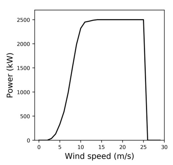
Figure 2.
Power curve of the design performance of a G114-2.5MW wind turbine used in the wind power ramp detection. The turbine has a cut-in wind speed of 3 m/s, a rated wind speed of 13 m/s, and a cut-out wind speed of 25 m/s.
Wind power variations are assumed to be only associated with meteorological conditions. Technical effects on the power output as yaw misalignment, response lag, and wakes of other wind turbines are not considered in this analysis. A wind power ramp is considered as a change in power greater than or equal to 20% of rated power in 1 h [43,44]. The positive (negative) rapid change in the wind power generation qualifies as a ramp up (down). The idea is to assess large wind ramps over the region. It is worth mentioning that the characteristics of wind ramps must consider relevant aspects for the end users of wind farms. According to previous studies [4,9], the number of ramp events becomes very sensitive to the threshold chosen. For this reason, a 30% capacity factor change in 1 h, was also used in the assessment. However, daily and monthly wind ramp distribution behaves similarly for both cases, even though fewer ramp events were identified for the higher power change (Figure S7, in supplementary material).
To improve comparability between observed and forecast winds, the latter were bilinearly interpolated to the weather station location and the 10 m wind speed was extrapolated to 80 m assuming the Monin-Obhukov similarity theory [39,40]. Then, wind speed was converted to wind power using the G114-2.5 MW power curve.
The comparison of the forecast with the observations was made for the 18-h forecast length in both models to make a fair comparison in terms of leading time (NAM contains hourly forecasts up to 36 h, then it has outputs every 3 h up to 84 h, while RAP has a horizon of 18 h). The time series of model forecast were constructed by concatenating sets of forecast with lengths going out 18 h for NAM and RAP models, similar to the independent forecast run method used by Bianco et al. [11]. The disadvantage of this approach is that discontinuities between the start and the end of each forecast run can create artificial ramps. However, a systematic creation of ramps was not detected. In addition, the errors of the series with the leading time did not show a clear increasing tendency.
Ramp metrics for events occurring in DJF and JJA in 2013 were calculated. Observed power changes that met the threshold but are not predicted are known as false negative (FN) (Figure S8a). A ramp produced by the model but not observed is defined as a false positive (FP) (Figure S8b). Finally, a ramp is considered as correctly forecasted (True positive: TP) if the threshold criterion is met in timing by the forecast and the observation (Figure S8c). The effect of relaxing the time threshold to 3 h was tested in the forecast.
The following forecast verification indices were calculated using a contingency table for observed and forecast ramp events: probability of detection (POD), frequency bias score (FBIAS) and False Alarm Rate (FAR) [45]. Their definitions are shown in Table 2.
Persistent high and low generation events were calculated for each weather station considering the instantaneous plant factor. Using the percentage of the hypothetical power obtained in one hour with respect to the nominal power of a wind turbine, the cumulative distribution of instantaneous plant factors, extreme events of high generation (99th percentile), moderate extreme events of high generation (90th percentile) and extreme events of low generation (20th percentile) were obtained.
3. Results and Discussion
This section details the topographic and climate characteristics of the four regions defined in Section 2.3.1. The effects of WS on the monthly and daytime variability of ramps and persistent generation events are discussed. Finally, a verification of the NAM and RAP forecast for wind, wind power ramps and persistent generation events is examined.
3.1. Study Regions
The stations were grouped for analysis considering the terrain morphology and WS in the region. The regions are: Plateau, Northeastern Mexico (NEMEX), Gulf of California (GoC) and Baja California Peninsula (BCP).
The Plateau is an arid-semiarid region (blue circles in Figure 1) extending from the United States border to the Trans-Mexican Volcanic Belt, and is bounded by the Sierra Madre Occidental and Sierra Madre Oriental to the west and east, respectively. The analysis described in Section 2.2 shows that local circulations develop in the region with a typical reversal of wind direction during the day in summer. However, winds are more intense in the winter associated with mid-latitude systems (Figure 3a,b). The weather stations included in this group are Ciudad Cuauhtemoc (CDCU), La Rumorosa (LARU), La Flor (LFLO) and Villa Ahumada (VAHU). The LARU station is not located over the Plateau region but is affected by WS similar to those affecting this group stations. Examination of wind power ramps and persistent events in Section 3.2.1 and Section 3.2.2 confirms this statement. Therefore, for the analysis of the wind characteristics due to WS, this station was included in the group Plateau.
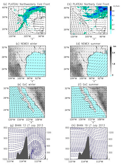
Figure 3.
Typical weather systems modulating wind power ramp variability over four different regions in Mexico. Topography, in km (grey shaded). Composite pattern of gradient of equivalent potential temperature (×10−2 K/km) and ERA5 surface wind as front position indicator (Plateau) for 2014–2015 during (a) westerly cold front and (b) northerly cold front; NEMEX surface wind climatology from 1979–2018 during (c) winter, (d) summer; BCP surface wind climatology from 1979–2018 during (e) winter, (f) summer; mean circulation on the x–z plane calculated with the NAM analysis model at (g) 1300 local time (LT) for July 2013, (h) 1900 LT for July 2013 at BHAN latitude (28.89° N).
NEMEX is a flat terrain region with maritime influence reaching even the Ocampo (OCAM) weather station over a mountain–coast transition. Wind intensification is caused by trade winds northward shifting in summer (Figure 3d); these moist winds blowing from the Gulf of Mexico persist from June to August. Meanwhile, cold fronts moving into the Gulf of Mexico produce intense northerly winds in the winter [36,46]. The group’s stations are OCAM, Santa Cecilia (SNCE) and Venustiano Carranza (VCAR), (yellow circles in Figure 1).
The Cabo Pulmo (CPUL) and El Pinacate (PINA) stations (green circles in Figure 1) were grouped together because the winds are associated with a predominantly synoptic circulation, northerly in winter and southerly during the summer (Figure 3e,f). The wind flowing between the mountainous systems Sierra La Laguna and the Sierra Madre Occidental, produces moderate channeled winds over the GoC. The Sierra La Laguna (SILA) station, located at the mountain (1949 m.a.s.l), is also shown in this group.
BCP region is an area that combines coasts with mountain systems such as Sierra La Laguna, where the highest peak reaches 2080 m.a.s.l. In this region characterized by the inhomogeneity of the land (composition and morphology), there are thermal circulations such as the sea-land breeze and katabatic winds, which can combine to produce intense winds (Figure 3g,h). The weather stations of this region are Bahia de los Angeles (BHAN), Bahia de Loreto (BHLO), Cabo San Lucas (CSNL) and San Juanico (NICO) (red circles in Figure 1).
3.2. Wind Power Variability
3.2.1. Wind Power Ramp Characterization
The intraseasonal variability of wind ramps is mainly modulated by synoptic-scale systems during winter (Figure 4) as a consequence of the increment of cold front incursions over Mexico. Their effects last between 2 and 6 days, depending on the phase speed [47]. In this dry season (October–April), the northerly intense cold air associated to frontal systems increases the occurrence of wind ramps, more evident in the Plateau (Figure 4a), GoC (Figure 4c) and BCP (Figure 4b) regions.
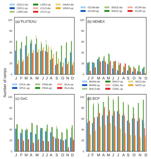
Figure 4.
Monthly mean of wind power ramp-up (dark color) and ramp-down (light color) events for (a) Plateau, (b) NEMEX, (c) GoC, (d) BCP regions.
Wind ramps are also generated by diurnal variations in wind intensity, which can be related to the establishment of local circulations such as sea-land and valley-mountain breezes as well as MCS, similar behavior has been found over USA arid regions [14]. The coastal and Plateau regions experience these WS mainly from March to July (Figure 4a,d, further explanation is given in Section 3.2.3). A ramp produced by storms occurs when the increase in wind speed coincides with the precipitation in the station (Figure S5).
For the four regions, the increase in ramp events at the beginning of the wet season is associated with MCS. These events are more frequent from June to August over Mexico [48]. The spatial distribution of the systems reported by [49] shows MCS events over the PLATEAU and NEMEX regions, especially frequent from April to August. Sudden changes in wind power production are less frequent towards the end of the wet season (September to November), (Figure 4). Furthermore, there is a symmetrical behavior of the wind power ramp-up and ramp-down events (Figure 4).
Generally, ramps-up are more frequent between 10:00–16:00 local time (LT) (Figure 5a–c) in most of the weather stations, probably as a result of diurnal variation of ground heating and its interaction with the atmospheric boundary layer. In the afternoon, the decrease of solar radiation reaching the surface attenuates horizontal thermal gradients, resulting in weaker winds. This transition occurs between 19:00–22:00 LT (Figure S3), producing a maximum of ramp-down events (Figure 5a–c).
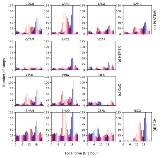
Figure 5.
Hourly distribution of annual mean wind power ramp-up (red) and ramp-down (blue) events for (a) Plateau, (b) NEMEX, (c) GoC, (d) BCP regions.
Different behavior is found in three stations over complex topography: CSNL, BHAN and SILA. In the first, a coastal area at the end of the Sierra La Laguna mountain range, the combination of local effects such as katabatic/land breeze circulation generates a second maximum on ramp-up frequency around 19:00 LT (Figure 5d). Otherwise, the frequency of wind power ramp-down is maximum from 7:00–10:00 LT due to the weakening of circulation driven by topography. Moreover, ramp-ups are more frequent at night in the hilly terrain of SILA station, when katabatic winds are set in.
3.2.2. Persistent High and Low Wind Power Generation Events
The maximum frequency of extreme high generation events in DJF and March–April–May (MAM) seasons is mainly caused by frontal systems passing over Northern Mexico. The satellite image (example in Figure S4) during the occurrence of an extreme event shows the frontal position over the deployed weather stations, as confirmed by a composite of gradient of equivalent potential temperature (Figure 3a,b). The annual distribution of extreme events varies spatially because frontal incursions come from the Pacific Ocean or from the north [35]. Some northerly winds affect just NEMEX and Plateau regions.
On the other hand, the maximum of extreme high generation events in JJA season is mainly associated to mesoscale systems, such as MCS. The northward shifting of trade winds during summer can favor the convection over NEMEX region [46]. Meanwhile, short generation events over Plateau and BCP are also related to thermal circulations.
Generally, extreme events of high generation are recurrent from March to August except for GoC stations. The intense winds in the latter are originated by frontal systems in DJF [50], leading to an increase in events of duration ≥3 h (Figure 6c). Moderate extreme events (not shown) are influenced by the same WS as extreme events.
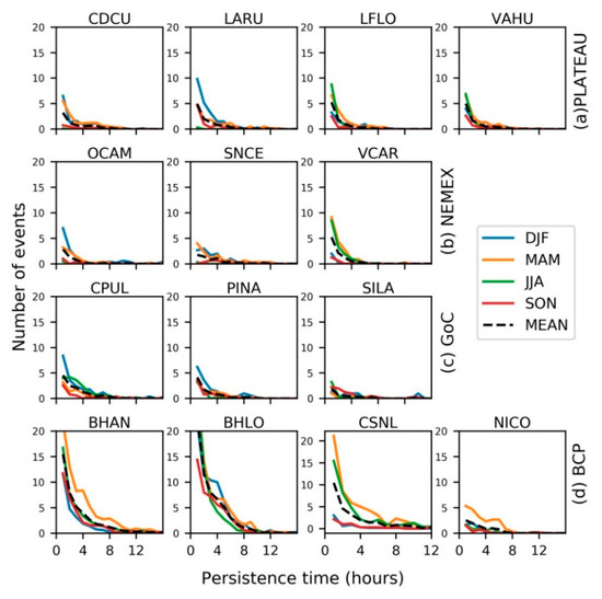
Figure 6.
Seasonal mean number of extreme persistent high generation events (99 percentile of Capacity Factor) for (a) Plateau, (b) NEMEX, (c) GoC, (d) BCP regions. March–April–May (MAM), June–July–August (JJA), September–October–November (SON), December–January–February (DJF).
Low generation events are more frequent from the end of the dry season to the beginning of the wet season, March to August months, for the four regions (details will be discussed in Section 3.3). For coastal regions, wind intensifies with the sea breeze establishment but the wind weakening during the transition to land breeze, gives place to periods of low generation. In addition, thunderstorm downdrafts can produce short high generation periods following by a low generation period when the storm ends (Figure S5), as observed in wind farms [51].
3.2.3. Weather Systems Underlying Wind Ramps
The average near-surface wind in Northern Mexico is weak (~4 m/s). The Plateau region experiences frontal systems to the end of the dry season, which leads to an increase in the average wind and the violin plot whiskers (Figure 7a). It is interesting to note that the moderate topographic gradients produce a bimodal wind behavior in LARU during summer (Figure 7) similar to that observed in coastal areas. Thermal circulations can be distinguished by two maxima in wind speed frequency, for example, in the sea-land breeze, there are a diurnal onshore wind and a nocturnal offshore wind.
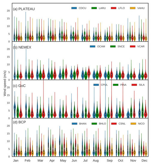
Figure 7.
Violin plots of monthly 10 m wind speed for (a) Plateau, (b) NEMEX, (c) GoC, (d) BCP. Violin plot include a white point for the median of the data and a box indicating the interquartile range. Whiskers indicate variability outside the first and third quartile and below 1.5 times interquartile range. Outliers extend out the whiskers. Distribution of the data is shown by a kernel distribution [52].
The trade winds over NEMEX (Figure 3d) at the beginning of the wet season increases the average monthly wind speed and decreases the number of extreme events (reflected by a shortening of the violin tails in Figure 7b). In contrast, during winter, the influence of mid-latitude systems causes large changes in the wind speed (more elongated violin whiskers).
The predominant mean wind in the GoC is northerly in the winter and southerly in summer (Figure 3a,b). The morphology of the terrain combined with the passage of cold fronts generates wind channeling (Figure 3a,b), and great wind speed variability (elongation of violin plot in Figure 7c). Extreme winds in the central and southern BCP and GoC are due to tropical cyclones, particularly in August and September, as revealed by the Pacific Hurricane season [53].
A weak synoptic forcing, in the summer, allows the enhancement of land-sea breeze in BCP which is reflected in a wind speed bimodal behavior and greater data dispersion (more elongated violin) (Figure 7d). The nocturnal component wind (without katabatic flow) is usually weaker, around 3 m/s, with respect to the diurnal sea-breeze component (~7 m/s), resulting in an increase in wind power ramp-up/down events (Figure 4d).
Synoptic systems control wind power ramp events over Northern Mexico. Frontal systems and trade winds usually persist for days over the affected regions. This characteristic enables the occurrence of longer extreme events of high generation compared to sites dominated by local circulations. In the latter, the reversal of wind direction due to the thermally driven circulations increases the frequency of short-lived events of low power generation (Figure S10a,d).
The WS acting on the four regions are summarized in Table 1. The areas are classified in terms of the atmospheric system that drives wind fluctuations in the dry and wet seasons as well as topography complexity.
Local circulations play an important role over complex terrain at the end of the dry season. Wind veering and return flow are observed in the coastal complex terrain of BCP (Figure 3e,f). The circulation is strong during summer due to greater contrast between sea and land temperatures, weak large-scale flow and clear skies [54]. Over continental areas in steeper terrain, the diurnal cycle of surface heating induces baroclinicity relative to the background air causing upslope flow at the daytime and downslope flows at night, as observed over the Plateau region. This effect can also enhance sea breeze circulation over complex terrain. Therefore, the representativeness of thermal circulations in the models is essential to reproduce the variability of the wind near the surface, which depends on the proper description of the topography and land cover [13,14].
3.3. NAM and RAP Wind Forecasting
3.3.1. Model Verification
The wind resource management requires not only the accurate prediction of wind but also that of sudden changes in wind power. The operational models, namely the NAM [27] and RAP [15] model systems, were used to assess the ability of wind forecast over the target region. A wind forecast evaluation is carried out in terms of ramp frequency and persistent high/low generation events. The 2013 forecast was selected for comparison purposes, due to the continuity and quality of the observed data during this year. Weather stations had around 98% of good quality records.
The Taylor diagram [55] summarizes the statistical parameters of correlation, standard deviation and centered root-mean-square (CRMS) difference for comparison. Wind forecasts that match the observations fall near the point on the x-axis called REF (Figure 8). The CRMS difference between forecast and observed winds is proportional to the distance to the point on the horizontal axis identified as REF. Semicircular contours indicate CRMS. At the REF point, the forecasts have a correlation of 1 and a standard deviation similar to that of the observations, which is interpreted as variations of the predicted variable of the same amplitude as observed.
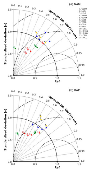
Figure 8.
Taylor diagram for (a) NAM and (b) RAP of forecast 10 m wind speed and observations at 14 weather stations grouped in regions: Plateau (blue dots), NEMEX (yellow dots), GoC (green dots) and BCP (red dots). The radial coordinate is the magnitude of the standard deviation, which is normalized by the standard deviation from observation and denoted by black dot lines. The concentric black semi-circles denote centered root-mean-square (CRMS) difference values. The angular coordinate shows the correlation coefficient (denoted by grey dot lines).
NAM and RAP forecast metrics show a similar distribution in the Taylor diagram. A correlation pattern by regions is not found, but standard deviation pattern is observed (Figure 8). For instance, for stations located on Plateau and NEMEX, the standardized deviation (σ) ranges from 0.9 to 1.1. The good forecast of wind variability in these regions is associated with the synoptic phenomena, cold fronts during the winter regime and set in of trade winds in NEMEX in summer. In the GoC region, the models show a decrease in this predictability (σ~0.8).
Low standardized deviation (<0.75) is observed over complex terrain regions in the BCP (Figure 8), showing a low variability of the wind forecast by both models compared to the observed wind variability. The model accuracy can be affected by the slope of the terrain, which in the case of sites like BHAN, is smoothed out by both models (Figure 9). The representativeness of the topographic forcing is a fundamental element to reproduce the magnitude and variability of the wind [56]. The thermally driven winds are generated by horizontal temperature gradients, derived from the spatial changes in the characteristics of the terrain such as elevation, soil cover and soil moisture [57]. The inadequate description of the land surface produces differences between the observed and predicted energy budget and the respective thermal contrast.
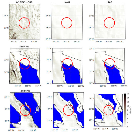
Figure 9.
GTOPO30 [32] slope and represented slope terrain by NAM and RAP around weather stations. The red circles are 50 km in radius centered at (a) CDCU, (b) PINA and (c) BHAN weather station.
The comparison between the observed and predicted 10 m wind shows that both models tend to overestimate weak winds and to underestimate strong winds (>8 m/s) (Figure 10b,c). The error is greater in weather stations with σ < 0.75 as shown in Figure 10c for BHAN. The underestimation of winds in the planetary boundary layer may result from misrepresentation of topographic slope by the models. For instance, as the air rises over a ridge, compression of air layers accelerates the wind [58]. If the model considers the terrain smoothed out, the wind acceleration will be decreased or non-existent, forecasting weaker winds than those observed [58].
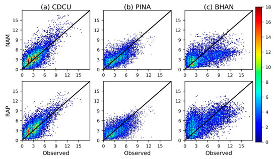
Figure 10.
Comparisons between the 10 m wind speed between observations and NAM and RAP models in 2013 for (a) CDCU (1.1 < σ <0.9), (b) PINA (σ~0.8), (c) BHAN (σ ≤ 0.75). The number of occurrences are shown in shaded.
The annual mean absolute error (MAE) and bias vary with the characteristics of the terrain (Table 3). Over the four regions, wind speed bias in RAP is smaller than in NAM. Bias patterns by regions were not found. BCP stations located on complex topography have a MAE greater than regions with moderate and flat topography (NEMEX). A small error in wind speed can imply a large error in wind power, for that reason MAE and Bias of wind power are evaluated (Table S1 in supplementary material). MAE wind power errors range from 274 kW to 827 kW, the greatest MAE values correspond to BCP stations, with exception of NICO, in concordance with wind speed errors. NAM MAE of wind power tends to be smaller or equal than RAP MAE. There is no clear MAE tendency to increase with lead time for both models.
Table 3.
Mean absolute error, bias and altitude difference for NAM and RAP in Plateau, NEMEX, GoC and BCP.
Jimenez and Dudhia [56] highlighted the deficiencies of the WRF model in wind forecast over regions of complex terrain, especially when there are significant differences between the actual and represented topography. An analysis of topography representativeness around the site of interest could give a deep insight into the role of topography than just considering the difference in altitude between the model and the weather station. Even if the site altitude is correct in the model, but the surrounding topography is not adequately represented (Figure 9), thermal forcing may not be captured by the models leading to an erroneous representation of local circulations and significant differences in the predicted wind (e.g., BHAN).
The valley-mountain and sea-land breeze are characterized by a diurnal inversion in the direction of flow. The accurate forecast wind direction can be a good indicator of the representation of local circulation by NAM and RAP. In general, the forecast wind direction by RAP is consistent with the observed, while NAM has deficiencies for some sites. For instance, NAM forecasts a land-sea breeze weaker than observed in BHAN (Figure 11c). Furthermore, mountains and hills can block or channel the wind. For instance, the absence of mountains in the topographic representation of the NAM at the northeast of PINA did not block flow from this direction, as is observed (Figure 11b).
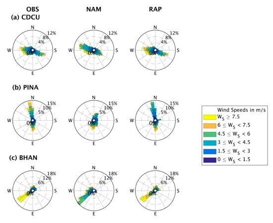
Figure 11.
2013 forecast and observed wind rose of hourly surface wind for (a) CDCU; (b) PINA; and (c) BHAN stations. For illustrative purposes only a good (1.1 < σ < 0.9), regular (0.9 ≤ σ < 0.75) and low wind predictability (σ ≤ 0.75) station, according to the Taylor diagrams (Figure 8), is shown.
3.3.2. Ramp Indices
Predicting sudden wind changes can be challenging for forecast models. A model with good skill to predict wind ramps has a POD and FBIAS near 1, and a FAR near zero. NAM and RAP models show low skill to predict ramp events at the observed timing span (low POD) over the four regions. Both forecast systems tend to under forecast (FBIAS < 1) ramp events. According to ramp indices, RAP performs better than NAM in both seasons (Figure 12). There is no clear improvement in forecasting events from summer to winter.
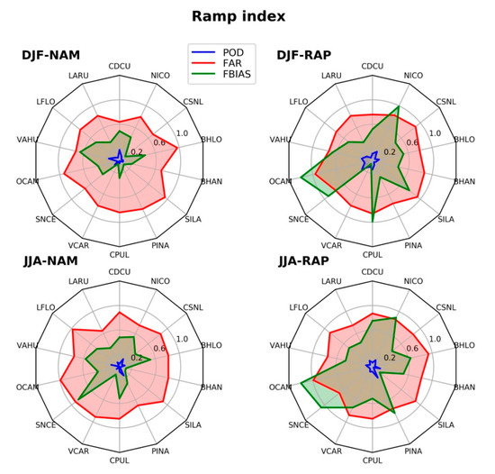
Figure 12.
2013 Seasonal Probability of detection (POD), False Alarm Rate (FAR) and Frequency Bias (FBIAS) metrics for forecast wind ramps by NAM and RAP models. Ramp event is defined as a variation of 20% in wind power in one hour.
The number of predicted and no-observed ramp-up events (FAR) by NAM is greater in summer than winter for NEMEX and some stations of the Plateau region (Figure 12). The establishment of trade winds on NEMEX increases the number of ramps predicted by both models, although there is no timing in the occurrence (low POD). No lag pattern was detected between observation and forecast.
Wind power ramps forecasting is improved by relaxing the time threshold for 3 h (Figure S9, in supplementary material), the number of corrected predictions increases (POD > 0.1) and the false predicted events are less frequent (FAR~0.7) in comparison to 1 h events.
The CSI is low (~0.1) for predicting power changes of 20% of rated power in 1 h over all the weather stations, which can be considered a strict threshold. Relaxing the time window, wind power ramps of the same magnitude occurring at 3 h are better predicted by NAM and RAP models. The RAP shows higher CSI than NAM, for most of the weather stations (Table 4).
Table 4.
2013 Critical Success Index (CSI) for wind power ramps in RAP and NAM models during December–January–February (DJF) and June–July–August (JJA) 2013. Ramps are power changes of 20% of rated power in 1 h or 3 h.
3.3.3. Forecast of High Generation Events
Observed and forecast high generation events show similar behavior, most of the events tend to last 1 h. However, the frequency of short duration events is underestimated by both NAM and RAP (Figure 13) for the four regions. Moderate short high generation events are markedly underpredicted in Plateau and BCP, probably as a result of a misrepresentation of the thermal circulations modulating the winds around the year. The models reproduce long-lasting events (greater than 4 h) fairly well, especially over the coast along NEMEX during the trade wind establishment (Figure 13b).
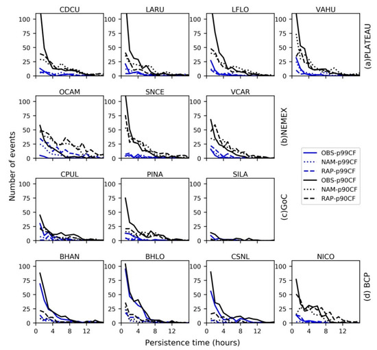
Figure 13.
Extreme events of high generation observed (continuous line), NAM (dotted line) and RAP (dashed line) for 2013. Moderate extreme events correspond to the 90th percentile (black line) of instantaneous capacity factor (CF). Regions are (a) Plateau, (b) NEMEX, (c) GoC, (d) BCP.
As mentioned in Section 3.3.1, the comparison between the observed and predicted 10 m wind shows that both models tend to overestimate the magnitude of weak winds and to underestimate the magnitude of strong winds (>8 m/s). Therefore, low persistent events are less frequently forecasted (underestimated) by the models for all weather stations (Figure S10, in supplementary material). The prediction of high and low generation events for NEMEX is fairly good. Overall, RAP performance is better than NAM for predicting extreme generation events.
In some cases, both models overestimate events lasting 5 h, since they are unable to capture sudden short events (lasting ≤1 h. Abrupt changes in wind speed are usually missed out by the models, resulting in longer persistent events (Figure 13). Similar underestimation in the number of short-lasting events and overestimation of long-lasting events has been found using data from the MERRA global reanalysis [17]. This was deemed due to the underestimation of high-frequency variability in the modeled data [17], which might be also present in NAM and RAP.
4. Conclusions
The efficient operation of a wind farm and its integration into the electricity grid depends on the proper evaluation of wind variability. Sharp and sudden changes in wind power (ramp events) are one of the biggest challenges the wind industry has to deal with. This paper examines daily and monthly distributions of ramp events in four regions of Northern Mexico, as well as seasonal low and high generation events. The regions are defined considering weather systems and terrain characteristics. Wind power ramp events are modulated by seasonal WS, which range from synoptic to local scale. Surface weather stations that experience thermal circulations, like those in the Plateau and BCP regions, have greater daily wind speed fluctuations and a greater occurrence of wind power ramps. Daily and monthly variations of wind ramps frequency in regions under the influence of trade winds are less pronounced. This characteristic implies less demanding management of wind power ramps. Moreover, the strength of trade winds on NEMEX in the summer leads to greater production of wind power during this part of the year. The GoC region seems to be suitable for wind farms deployment because there is persistence of 10 m wind speeds >3 m/s throughout the year (Figure 7c) and few monthly wind ramps.
Frontal and MCS are the main drivers of persistent events. Long-lasting high generation events are typical of trade winds and front passages. Meanwhile, short-lasting events of high generation are more frequent in regions experiencing thermal circulations (e.g., Plateau and BCP), and low generation events are numerous due to transitions between nocturnal and diurnal circulation.
The identification of meteorological phenomena causing wind power ramps and persistent generation events shows aspects that should be considered in the design and development of a wind power ramp forecasting system. Microscale and mesoscale processes become relevant in sudden variations in wind power output of a single wind farm, especially over complex topography. Thermally driven circulations and storms are mesoscale events, with a horizontal extension ranging from 2 to 20 km, so they can affect a single wind farm with sudden variations in wind production. Otherwise, wind ramps of aggregate wind energy production in large areas (where groups of wind farms are distributed) are induced by synoptic phenomena such as cold fronts.
The forecasting models NAM and RAP show low ability to forecast wind variability over complex terrain (MAE > 2.0 m/s; σ ≤ 0.75) and tend to underestimate intense winds and to overestimate weak winds, resulting in a general underestimation of high and low generation events. However, the models are able to capture long-lasting generation events with durations between 5 and 10 h. Therefore, a forecasting system for a specific wind farm must consider the atmospheric processes that originate wind ramps and high/low generation events. Northern Mexico is located in a subtropical–tropical transition region and over complex topography, so the interaction between atmospheric and topographic forcing implies further difficulties in examining variability and wind ramps in observations and models. The scale of atmospheric phenomena will define the horizontal and vertical resolution necessary for modeling as well as the configuration of physical processes settings. Evaluating whether the state-of-the-art numerical weather prediction models are able to capture ramp features accurately, as shown in this study, can be used for model validations and improvements.
Supplementary Materials
The following are available online at https://www.mdpi.com/2073-4433/11/12/1281/s1, Figure S1: Weather stations (red dot) used in the study and wind farms (black star) in operation over Mexico, Figure S2: All day (a,d,g,j), day (b,e,h,k) and night (c,f,i,l) surface windroses from CPUL and BHAN weather stations for June–July–August (JJA) and December–January–February (DJF), Figure S3: Diurnal variations of the horizontal surface vector for CPUL (a,b) and BHAN (c,d) weather station in June–July–August (JJA) and December–January–February(DJF), Figure S4: Cold front over Northern Mexico in 13 January 2013 during a ramp event in PLATEAU region. A cold front is seen as a curving line of clouds in the MODIS Corrected Reflectance imagery, Figure S5: Meteogram at CDCU for a storm of 21 July 2012, Figure S6: Example of summer ramp-up event at Ciudad Cuauhtémoc (red circle) in 21 July 2012. ERA5 surface wind speed and CMORPH daily precipitation in mm (shaded), Figure S7: Monthly mean of wind power ramp-up (dark color) and ramp-down (light color) events for (a) Plateau, (b) NEMEX, (c) GoC, (d) BCP regions. Ramp is a change of 30% or greater in rated power in 1 h, Figure S8: Example of wind power ramps (≥20% of rated power) (a) observed but not predicted, (b) predicted by RAP but not observed in one hour and (c) predicted by RAP and observed in 3 hours. Capacity factor is the ratio between the power generation and the rated power, Table S1: Wind power forecast Mean Absolute Error (MAE) and Bias error for 14 weather stations in 2013. Errors are in kW. Wind power was derived by extrapolating NAM, RAP and observation to 80 m and using the G114-2.5 wind power curve, Figure S9: POD, FAR and FBIAS metrics for a variation ≥20% of rated power in 3 hours for June–July–August (JJA) and December–January–February (DJF) 2013, Figure S10: Extreme events of low generation observed (continuous line), NAM (dotted line) and RAP (dashed line) for 2013. Extreme events correspond to the 20th percentile (black line) of instantaneous capacity factor (CF). Regions are (a) Plateau, (b) NEMEX, (c) GoC, (d) BCP.
Author Contributions
Conceptualization, K.P.-C. and E.C.; methodology, K.P.-C.; formal analysis, K.P.-C.; investigation, K.P.-C.; data curation, K.P.-C.; writing—original draft preparation, K.P.-C.; writing—review and editing, E.C., O.M.-A., A.L.Q.-M.; supervision, E.C. All authors have read and agreed to the published version of the manuscript.
Funding
This research was funded by The National Council of Science and Technology (CONACYT), grant number 473276 the first author’s PhD scholarship. OM-A’s contribution was funded by the UK National Centre for Atmospheric Science (NCAS) through the Atmospheric hazard in developing Countries: Risk assessment and Early Warning (ACREW) project (NE/R000034/1).
Acknowledgments
The authors are grateful to Edgar Dolores Tesillos for preparing the first figure.
Conflicts of Interest
The authors declare no conflict of interest. The funders had no role in the design of the study; in the collection, analyses, or interpretation of data; in the writing of the manuscript, or in the decision to publish the results.
References
- SENER. Programa de Desarrollo del Sistema Eléctrico Nacional 2015–2029; Secretaría de Energía: Ciudad de México, México, 2015; Available online: https://www.gob.mx/sener/acciones-y-programas/programa-de-desarrollo-del-sistema-electrico-nacional-33462 (accessed on 24 September 2020).
- DeCesaro, J.; Porter, K.; Milligan, M. Wind energy and power system operations: A review of wind integration studies to date. Electr. J. 2009, 22, 34–43. [Google Scholar] [CrossRef]
- Greaves, B.; Collins, J.; Parkes, J.; Tindal, A. Temporal forecast uncertainty for ramp events. Wind. Eng. 2009, 33, 309–319. [Google Scholar] [CrossRef]
- Gallego-Castillo, C.; Cuerva-Tejero, A.; Lopez-Garcia, O. A review on the recent history of wind power ramp forecasting. Renew. Sustain. Energy Rev. 2015, 52, 1148–1157. [Google Scholar] [CrossRef]
- Cutler, N.; Kay, M.; Jacka, K.; Nielsen, T.S. Detecting, categorizing and forecasting large ramps in wind farm power output using meteorological observations and WPPT. Wind. Energy 2007, 10, 453–470. [Google Scholar] [CrossRef]
- Bossavy, A.; Girard, R.; Kariniotakis, G. Forecasting Uncertainty Related to Ramps of Wind Power Production. In Proceedings of the European Wind Energy Conference and Exhibition 2010 (EWEC 2010), Warsaw, Poland, 20–23 April 2010; Curran Associates: Reed Hook, NY, USA, 2010; Volume 2, p. 9, ISBN 9781617823107. hal-00765885. [Google Scholar]
- Kamath, C. Associating weather conditions with ramp events in wind power generation. In Proceedings of the 2011 IEEE/PES Power Systems Conference and Exposition, Phoenix, AZ, USA, 20–23 March 2011; pp. 1–8. [Google Scholar] [CrossRef]
- Yang, Q.; Berg, L.K.; Pekour, M.; Fast, J.D.; Newsom, R.K.; Stoelinga, M.; Finley, C. Evaluation of WRF-predicted near-hub-height winds and ramp events over a Pacific Northwest site with complex terrain. J. Appl. Meteorol. Clim. 2013, 52, 1753–1763. [Google Scholar] [CrossRef]
- Gallego, C.; Cuerva, A.; Costa, A. Detecting and characterising ramp events in wind power time series. J. Physics: Conf. Ser. 2014, 555, 012040. [Google Scholar] [CrossRef]
- Cui, M.; Zhang, J.; Florita, A.R.; Hodge, B.-M.; Ke, D.; Sun, Y. An optimized swinging door algorithm for identifying wind ramping events. IEEE Trans. Sustain. Energy 2016, 7, 150–162. [Google Scholar] [CrossRef]
- Bianco, L.; Djalalova, I.V.; Wilczak, J.M.; Cline, J.; Calvert, S.; Konopleva-Akish, E.; Finley, C.; Freedman, J. A wind energy ramp tool and metric for measuring the skill of numerical weather prediction models. Weather. Forecast. 2016, 31, 1137–1156. [Google Scholar] [CrossRef]
- Smith, N.H.; Ancell, B.C. Variations in parametric sensitivity for wind ramp events in the Columbia river basin. Mon. Weather. Rev. 2019, 147, 4633–4651. [Google Scholar] [CrossRef]
- Siuta, D.; West, G.; Stull, R. WRF Hub-height wind forecast sensitivity to PBL scheme, grid length, and initial condition choice in complex terrain. Weather. Forecast. 2017, 32, 493–509. [Google Scholar] [CrossRef]
- Deppe, A.J.; Gallus, W.A.; Takle, E.S. A WRF Ensemble for improved wind speed forecasts at turbine height. Weather. Forecast. 2013, 28, 212–228. [Google Scholar] [CrossRef]
- Benjamin, S.G.; Weygandt, S.S.; Brown, J.M.; Hu, M.; Alexander, C.R.; Smirnova, T.G.; Olson, J.B.; James, E.P.; Dowell, D.C.; Grell, G.A.; et al. A North American hourly assimilation and model forecast cycle: The rapid refresh. Mon. Weather. Rev. 2016, 144, 1669–1694. [Google Scholar] [CrossRef]
- Archer, C.L.; Colle, B.A.; Monache, L.D.; Dvorak, M.J.; Lundquist, J.K.; Bailey, B.H.; Beaucage, P.; Churchfield, M.J.; Fitch, A.C.; Kosovic, B.; et al. Meteorology for coastal/offshore wind energy in the united states: Recommendations and research needs for the next 10 years. Bull. Am. Meteorol. Soc. 2014, 95, 515–519. [Google Scholar] [CrossRef]
- Cannon, D.; Brayshaw, D.; Methven, J.; Coker, P.; Lenaghan, D. Using reanalysis data to quantify extreme wind power generation statistics: A 33 year case study in Great Britain. Renew. Energy 2015, 75, 767–778. [Google Scholar] [CrossRef]
- Musilek, P.; Li, Y. Forecasting of wind ramp events-Analysis of cold front detection. In Proceedings of the 31st International Symposium on Forecasting, Prague, Czech Republic, 26–29 June 2011. [Google Scholar]
- Ohba, M.; Kadokura, S.; Nohara, D. Impacts of synoptic circulation patterns on wind power ramp events in East Japan. Renew. Energy 2016, 96, 591–602. [Google Scholar] [CrossRef]
- Sherry, M.; Rival, D.E. Meteorological phenomena associated with wind-power ramps downwind of mountainous terrain. J. Renew. Sustain. Energy 2015, 7, 033101. [Google Scholar] [CrossRef]
- Walton, R.A.; Gallus, W.A.; Takle, E.S. Wind ramp events at turbine height-spatial consistency and causes at two Iowa wind farms. In Proceedings of the 4th Conference Weather, Climate, New Energy Economy, Austin, TX, USA, 5–10 January 2013; pp. 1–7. [Google Scholar]
- Colle, B.A.; Mass, C.F. The structure and evolution of cold surges east of the Rocky Mountains. Mon. Weather. Rev. 1995, 123, 2577–2610. [Google Scholar] [CrossRef]
- Fitzjarrald, D.R. Slope wind in Veracruz. J. Clim. Appl. Meteorol. 1986, 25, 133–144. [Google Scholar] [CrossRef]
- Carvalho, D.; Rocha, A.; Gómez-Gesteira, M.; Santos, C.S. A sensitivity study of the WRF model in wind simulation for an area of high wind energy. Environ. Model. Softw. 2012, 33, 23–34. [Google Scholar] [CrossRef]
- Carvalho, D.; Rocha, A.M.A.C.; Gómez-Gesteira, M.; Santos, C.S. Sensitivity of the WRF model wind simulation and wind energy production estimates to planetary boundary layer parameterizations for onshore and offshore areas in the Iberian Peninsula. Appl. Energy 2014, 135, 234–246. [Google Scholar] [CrossRef]
- Draxl, C.; Hahmann, A.N.; Peña, A.; Giebel, G. Evaluating winds and vertical wind shear from Weather Research and Forecasting model forecasts using seven planetary boundary layer schemes. Wind. Energy 2014, 17, 39–55. [Google Scholar] [CrossRef]
- Rogers, E.; DiMego, G.; Black, T.; Ek, M.; Ferrier, B.; Gayno, G.; Janjic, Z.; Lin, Y.; Pyle, M.; Wong, V. The NCEP North American mesoscale modeling system: Recent changes and future plans. In Proceedings of the 23rd Conference on Weather Analysis and Forecasting and 19th Conference on Numerical Weather Prediction, Omaha, NE, USA, 1–5 June 2009; p. 2A.4. [Google Scholar]
- Hernandez-Escobedo, Q.; Manzano-Agugliaro, F.; Zapata-Sierra, A. The wind power of Mexico. Renew. Sustain. Energy Rev. 2010, 14, 2830–2840. [Google Scholar] [CrossRef]
- James, E.P.; Benjamin, S.G.; Marquis, M. A unified high-resolution wind and solar dataset from a rapidly updating numerical weather prediction model. Renew. Energy 2017, 102, 390–405. [Google Scholar] [CrossRef]
- Li, A.K.; Paek, H.; Yu, J.-Y. The changing influences of the AMO and PDO on the decadal variation of the Santa Ana winds. Environ. Res. Lett. 2016, 11, 64019. [Google Scholar] [CrossRef]
- Bingoel, F. Complex Terrain and Wind Lidars. Ph.D. Thesis, Technical University of Denmark, Risoe National Laboratory for Sustainable Energy, Roskilde, DK, USA, 2019. [Google Scholar]
- USGS 30 ARC-second Global Elevation Data, GTOPO30 1997; USGS: Reston, VA, USA, 1997. [CrossRef]
- Skamarock, W.C.; Klemp, J.B.; Dudhia, J.; Gill, D.O.; Barker, D.M.; Duda, M.G.; Huang, X.Y.; Wang, W.; Powers, J.G. A description of the advanced research WRF Version 3, mesoscale and microscale meteorology division. Natl. Cent. Atmos. Res. Boulder Color. USA 2008, 88, 7–25. [Google Scholar]
- Wu, W.-S.; Purser, R.J.; Parrish, D.F. Three-dimensional variational analysis with spatially inhomogeneous covariances. Mon. Weather. Rev. 2002, 130, 2905–2916. [Google Scholar] [CrossRef]
- Henry, W.K. Some aspects of the fate of cold fronts in the gulf of Mexico. Mon. Weather. Rev. 1979, 107, 1078–1082. [Google Scholar] [CrossRef][Green Version]
- Perez, E.P.; Magana, A.V.; Caetano, E.; Kusunoki, S. Cold surge activity over the Gulf of Mexico in a warmer climate1. Front. Earth Sci. 2014, 2. [Google Scholar] [CrossRef]
- Dominguez, C.; Done, J.M.; Bruyère, C.L. Easterly wave contributions to seasonal rainfall over the tropical Americas in observations and a regional climate model. Clim. Dyn. 2019, 54, 191–209. [Google Scholar] [CrossRef]
- Hersbach, H.; Bell, B.; Berrisford, P.; Hirahara, S.; Horányi, A.; Muñoz-Sabater, J.; Nicolas, J.; Peubey, C.; Radu, R.; Schepers, D.; et al. The ERA5 global reanalysis. Q. J. R. Meteorol. Soc. 2020, 146, 1999–2049. [Google Scholar] [CrossRef]
- Monin, A.S.; Obukhov, A.M. Basic Laws of Turbulent Mixing in the Atmosphere near the Ground. Tr. Akad. Nauk SSSR Geofiz. Inst. 1954, 24, 163–187. [Google Scholar]
- Stull, R. An Introduction to Boundary Layer, 1st ed.; Kluwer Academic Publishers: Dordrecht, The Netherlands, 2013; p. 666. [Google Scholar]
- International Electrotechnical Commission. Wind Turbines-Part. 1: Design Requirements, IEC 614001, 3rd ed.; International Electrotechnical Commission: Geneva, Switzerland, 2005. [Google Scholar]
- Hernández-Escobedo, Q.; Saldaña-Flores, R.; Rodríguez-García, E.; Manzano-Agugliaro, F. Wind energy resource in Northern Mexico. Renew. Sustain. Energy Rev. 2014, 32, 890–914. [Google Scholar] [CrossRef]
- Kamath, C. Understanding wind ramp events through analysis of historical data. In Proceedings of the IEEE PES T&D 2010, Sao Paolo, Brazil, 8–10 November 2010; pp. 1–6. [Google Scholar]
- Bradford, K.T.; Carpenter, R.L.; Shaw, B.L. Forecasting southern plains wind ramp events using the WRF Model At 3-Km. In Proceedings of the 9th Annual Student Conference of the American Meteorological Society, Atlanta, GA, USA, 16 January 2010; pp. 1–10. [Google Scholar]
- Wilks, D.S. Statistical Methods in the Atmospheric Science, 2nd ed.; Elsevier: Burlington, MA, USA, 2006; ISBN 0-12-064490-8. [Google Scholar]
- Magaña, V.; Amador, J.A.; Medina, S. The midsummer drought over Mexico and Central America. J. Clim. 1999, 12, 1577–1588. [Google Scholar] [CrossRef]
- Schultz, D.M.; Bracken, W.E.; Bosart, L.F. Planetary-and synoptic-scale signatures associated with Central American cold surges. Mon. Weather. Rev. 1998, 126, 5–27. [Google Scholar] [CrossRef]
- Manzanilla, A.V. Mesoscale convective systems in NW Mexico during the strong ENSO events of 1997–1999. Atmósfera 2015, 28, 143–148. [Google Scholar] [CrossRef]
- Manzanilla, A.V.; Vázquez, M.C.; Francisco, J.J.P. Un estudio explorativo de los Sistemas Convectivos de Mesoescala de Mexico. Investig. Geográficas 2012, 26. [Google Scholar] [CrossRef]
- Badan-Dangon, A.; Dorman, C.E.; Merrifield, M.A.; Winant, C.D. The lower atmosphere over the Gulf of California. J. Geophys. Res. Space Phys. 1991, 96, 16877–16896. [Google Scholar] [CrossRef]
- Zhang, S.; Solari, G.; De Gaetano, P.; Burlando, M.; Repetto, M.P. A refined analysis of thunderstorm outflow characteristics relevant to the wind loading of structures. Probabilistic Eng. Mech. 2018, 54, 9–24. [Google Scholar] [CrossRef]
- Parzen, E. On Estimation of a probability density function and mode. Ann. Math. Stat. 1962, 33, 1065–1076. [Google Scholar] [CrossRef]
- Martinez-Sanchez, J.; Cavazos, T. Eastern Tropical Pacific hurricane variability and landfalls on Mexican coasts. Clim. Res. 2014, 58, 221–234. [Google Scholar] [CrossRef]
- Morales-Acuña, E.; Torres, C.R.; Linero-Cueto, J.R. Surface wind characteristics over Baja California Peninsula during summer. Reg. Stud. Mar. Sci. 2019, 29, 100654. [Google Scholar] [CrossRef]
- Taylor, K.E. Summarizing multiple aspects of model performance in a single diagram. J. Geophys. Res. Space Phys. 2001, 106, 7183–7192. [Google Scholar] [CrossRef]
- Jiménez, P.A.; Dudhia, J. Improving the representation of resolved and unresolved topographic effects on surface wind in the WRF model. J. Appl. Meteorol. Clim. 2012, 51, 300–316. [Google Scholar] [CrossRef]
- Parker, D.J. Mesoescale meteorology overview. Encycl. Atmos. Sci. 2015, 316–322. [Google Scholar] [CrossRef]
- Zardi, D.; Whiteman, C.D. Diurnal mountain wind systems. In Mountain Weather Research and Forecasting; Chow, F., De Wekker, S., Snyder, B., Eds.; Springer: Dordrecht, The Netherlands, 2013; pp. 35–119. ISBN 978-94-007-4098-3. [Google Scholar]


Publisher’s Note: MDPI stays neutral with regard to jurisdictional claims in published maps and institutional affiliations. |
© 2020 by the authors. Licensee MDPI, Basel, Switzerland. This article is an open access article distributed under the terms and conditions of the Creative Commons Attribution (CC BY) license (http://creativecommons.org/licenses/by/4.0/).