Exposure Indices of Extreme Wind-Driven Rain Events for Built Heritage

Abstract

Building performance and material change of cultural heritage in urban areas are negatively impacted by wind-driven rain (WDR). The frequency and intensity of WDR exposure are modified by climate change. Current approaches to exposure assessment emphasise prolonged exposure. Here, we propose indices to represent the exposure of cultural heritage to extreme WDR events. The indices are derived in two stages: (1) time-binning of long-term exposure, and (2) statistical representation of the occurrence of infrequent but intense events by fitting to the Generalised Extreme Value (GEV) distribution. A comparison to an existing exposure assessment procedure demonstrates that the proposed indices better represent shorter, more intense, and more consistent WDR events. Indices developed for seasons had greater statistical confidence than those developed for annual exposure. One index is contextualised within a model of a gutter on a terraced building: this converts the index from a measure of exposure to potential impact. This evaluation demonstrated the importance of maintenance to reduce the potential impact of WDR events. This work has direct and indirect implications for developing robust assessment procedures for cultural heritage exposure to extreme weather events.

1. Introduction

Masonry walls have a high moisture content and are inherently wet to a greater or lesser extent. Historic masonry walls and their mortars have the ability to absorb and evaporate moisture provided foundations are not permanently saturated by rising damp or walls wetted by ineffective guttering. These effects, and the risk from wind-driven rain, were highlighted in a study of Brodick Castle, a 13th century sandstone Category A listed building on the Isle of Arran [1] (pp. 2–3). The study reported on the effects on wall moisture content of the failure of lead guttering and while adequate and well maintained rainwater disposal systems are at the heart of historic building protection, the increase in extreme episodic wind-driven rain events has highlighted the importance of impact indices and risk assessment to effective building maintenance and urban heritage management.

Time-binning is an integral part of assessing exposure to wind-driven rain. A set of rules and conditions are applied to a data series to produce an ordered set of discrete units (events), to which statistical analysis is applied. These units are indices that are intended to represent specific responses of built heritage to the environment. To date, time-binning of wind-driven rain time series have favoured “the average moisture content of exposed building material or when assessing the likely growth of mosses and lichens” [2] (p. 4) and “rain penetration through masonry” [3] (p. 12). These indices are derived from time-binning rules informed by the time scales of associated physical processes.

Time-binning is often combined with extreme value analysis (EVA) [4]. The units (wind-driven rain events) are fitted to an appropriate statistical distribution [5]. This enables the determination of statistical frequency (e.g., return periods), which can be projected far beyond the time scales of the input data. One challenge of EVA is how to interpret the statistical frequency of events. The output of time-binning and EVA primarily represent the intensity of events that built heritage is exposed to. However, what does a once-in-any-given 50-year period event represent in terms of risk to built heritage? The Noah’s Ark project—a collaborative EU project—developed and visualised several such indices (referred to as ‘Heritage Climate maps’) in the context of a changing climate [6]. However, rain events were not parameterised. An open challenge remains to produce representations of impact from statistical measures of rain events.

Current indices do not represent exposure to short but intense WDR events [3] (p. v). Primary concerns during these events include rain penetration through building elements (e.g., window frames, cracks, etc.) and the failure of rainwater goods (e.g., overspilling of gutters). Gutter overspill can result in substantial volumes of water to run off the façade of the building which can activate and foster several weathering mechanisms [7]. It is important to note that the relationship between surface run-off and absorption is complicated: for example, recent work [8,9] demonstrates that, after initial uptake, subsequent exposure may not result in significant change of moisture at depth in the walls.

The need for a new index that characterises shorter, more intense, and more consistent wind-driven rain events is evidenced by the damage that can be caused by rapid wetting and drying of the built heritage. For example, wetting dissolves salts presents in building materials and mortars. The speed of drying after a wetting episode can cause salt crystals to form either on or close to the surface of a material, leading to a variety of damage mechanisms such as disfiguring efflorescence, flaking, and spalling.

This paper proposes two new indices for exposure of built heritage to intense wind-driven events. The time-binning procedure is outlined, the output of which is compared to the intensity and temporal characteristics of indices in current use. These indices are derived from extreme value analysis, one of which is contextualised in a model of gutter overflow to represent potential impact on built heritage. The discussion that follows emphasises the combined use of these indices and contextualisation as a tool for comparative evaluation of impact assessment.

2. Results

2.1. Regional Case Study: Plymouth

Measured hourly climate data from Plymouth, UK (50.3544°, −4.11986°) from 1986–2015 was used to demonstrate and evaluate the time-binning procedure [10,11]. Plymouth is a port city situated on the south coast of England. Although there are very few pre-war buildings in the city centre due to extensive bombing during WWII [12], the fabric of the city includes extensive post-war rebuilding and terraced housing of various periods in the surrounding urban and peri-urban regions. This urban fabric is a tapestry of built heritage and an important representation of Britain’s participation in 20th-century international conflict.

Due in part to its exposed coastal setting, Plymouth experiences intense weather events. Recently, the Met Office recorded that winds reached 83 miles per hour during a storm [13]. Previous work has identified that one once-in-every-three-years wind-driven rain event (based on time-binning rules in ISO 15927-3:2009 [3]) can represent nearly 50% of the average annual exposure [14].

For the purposes of demonstrating the procedure and output of the proposed index for extreme events, a façade oriented to the southwest without any obstructions was used to determine the wind-driven rain exposure from measured climate data.

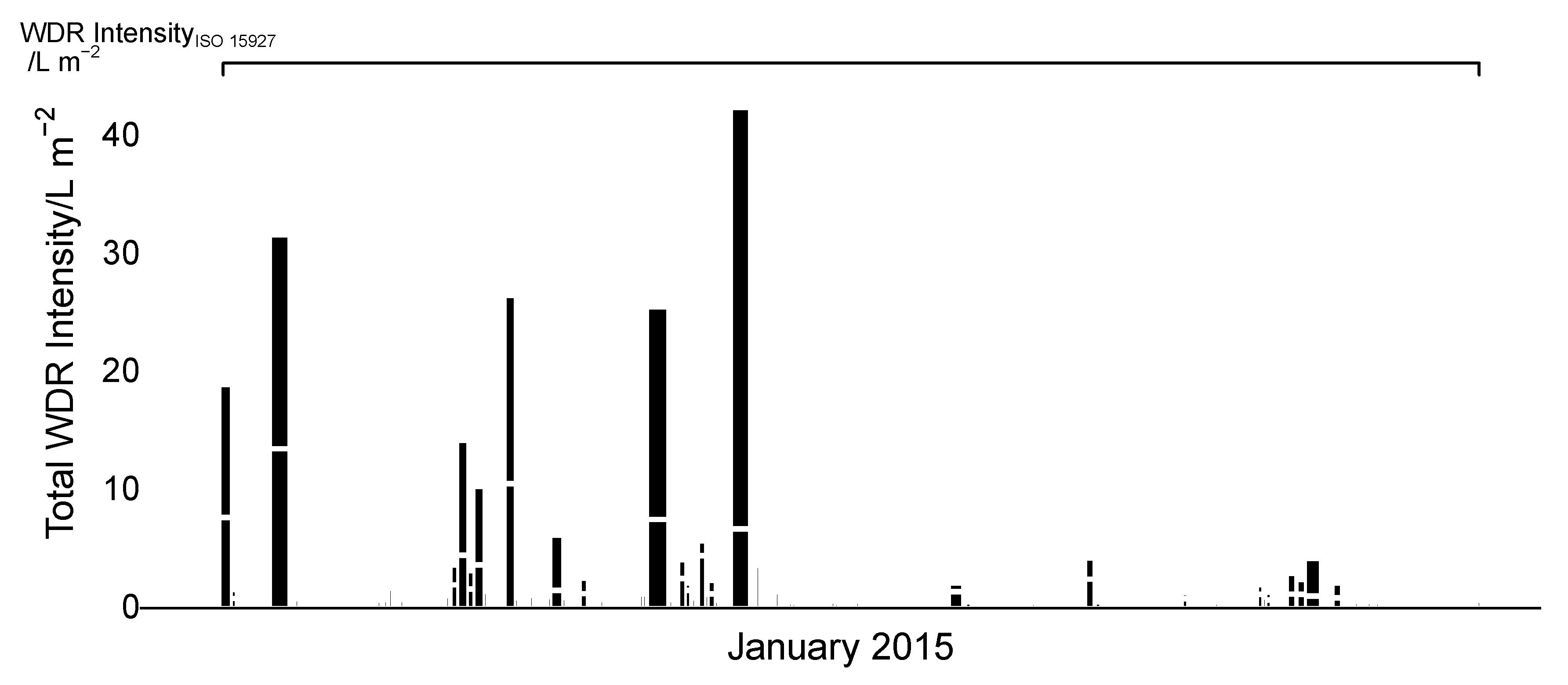
2.2. A Demonstrative Example

Current indices for wind-driven rain commonly applied to heritage may not represent short periods of intense exposure, while incorporating substantial periods without exposure. These characteristics are demonstrated using one month of exposure (Figure 1). In Plymouth, UK, 122.8 mm of precipitation was recorded in January 2015. For a façade oriented toward the southwest without any obstructions, this equates to a semi-empirical estimation (based on ISO 15927 [3]) of total wind-driven rain intensity equal to approximately 226 L m⁻².

Using the time-binning rules for prolonged events [3], the entire month is binned into one unit: a single wind-driven rain event. Applying a time-binning procedure that applies shorter criteria for the periods between events produces 64 events (1–15 h in duration) within the same month, of which the majority are less than 3 h in duration. These events range in intensity, but several represent more than 10% of the total wind-driven rain exposure for the month in a period of a few hours.

Current indices commonly represent periods of time in which periods of exposure are a small fraction of the total duration. Under the rules for prolonged exposure, approximately 20% of the hours within the event include wind-driven rain exposure. Under the proposed time-binning procedure for extreme events, each event that occurred in January 2015 has wind-driven rain exposure during each hour of their duration.

The maximum hourly intensity within each event varies. In the cases of events that are the duration of the data resolution (1 h), the average intensity is equal to the maximum hourly intensity. As the event duration increases (the maximum was 15 h in January 2015), the maximum hourly intensity as a fraction of the total within the event decreases. However, as can be seen in Figure 1, it commonly represents a third to a half of the total intensity of the event.

Thus, the characteristics of the wind-driven rain exposure within this month demonstrate that indices in current common use for prolonged events do not represent intense, short, and more consistent wind-driven rain events. In contrast, time-binning rules based on shorter periods between events characterises these phenomena when applied to hourly wind-driven rain exposure.

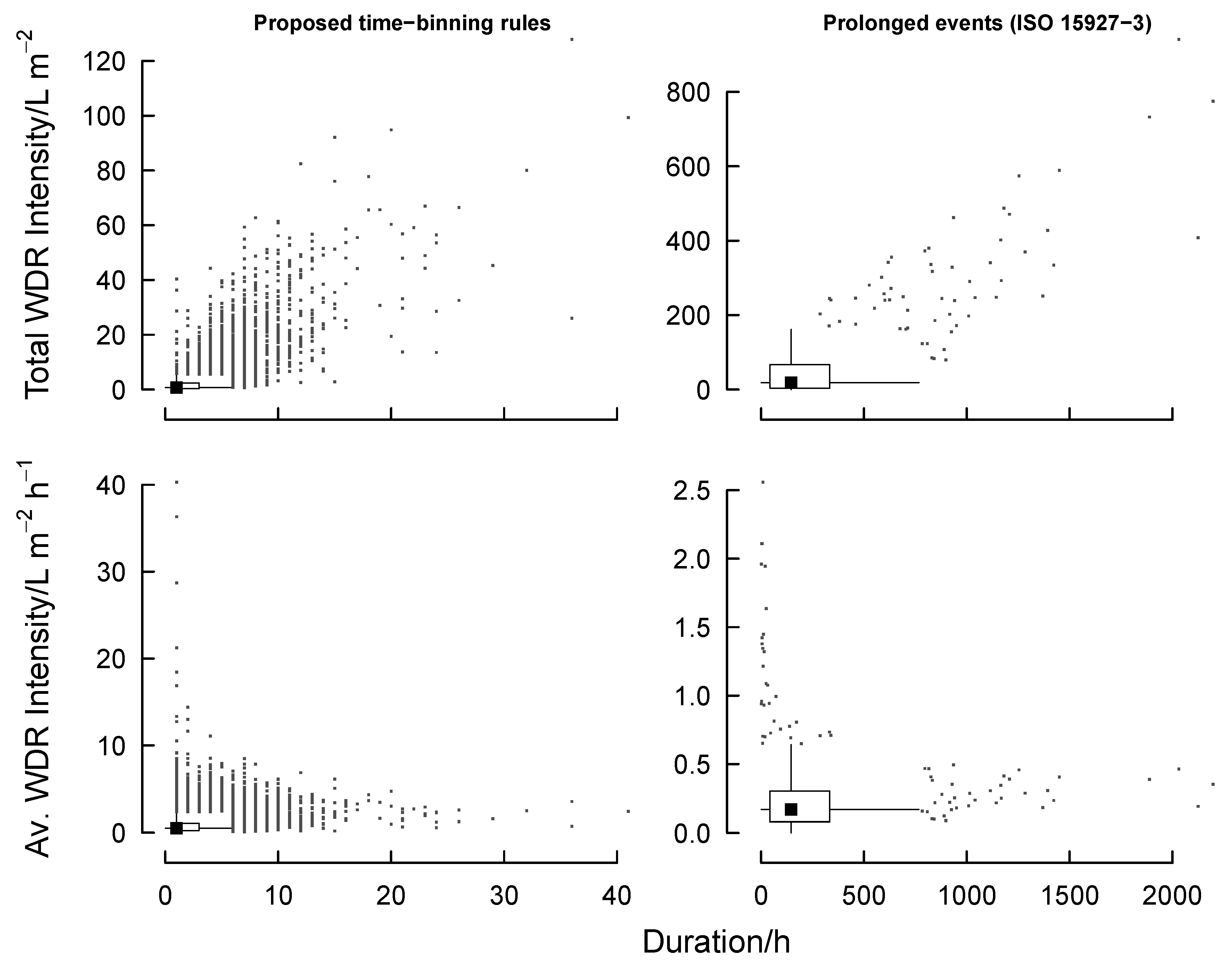
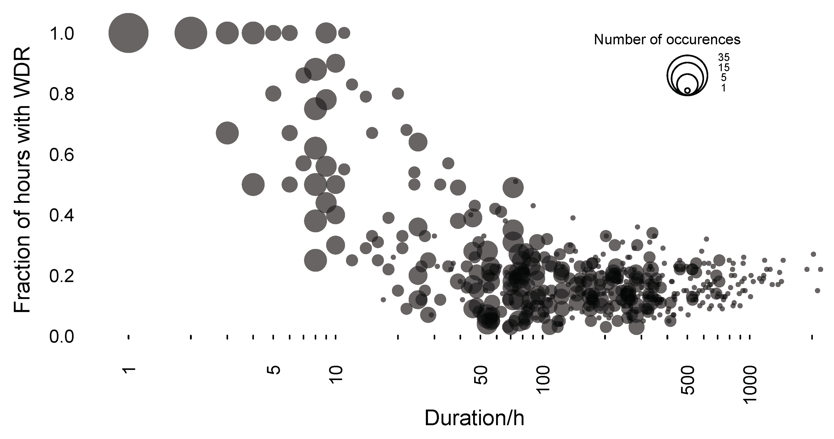
2.3. Temporal Characteristics of the Time-Binned Events

2.3.1. Intensity, Duration, and Maxima

The proposed time-binning rules produce shorter wind-driven rain events. Figure 2 shows that the durations of events under the proposed time-binning rules are, both on average and in their extreme, at least one order of magnitude less than those produced from rules for prolonged events. The former produce events up to 40 h in duration, although 95% of the events are less than 7 h in duration. In contrast, the prolonged events have a median duration of 146 h, with outliers (of the median + 1.5 × IQR, the inter-quartile range) between 850 and 2500 h in duration.

Events characterised by these sets of rules experience similarly-proportioned wind-driven rain exposure (Figure 2, upper row). The short events are primarily characterised by near-zero total (summed) intensities, with outlying events ranging from 0 to 130 L m⁻². The prolonged events primarily range between 0 and 200 L m⁻², but can reach upwards of 700 L m⁻². In both cases, there is a general proportionality between duration and intensity.

A different picture emerges when observing average intensity (Figure 2, lower row). In most cases, both sets of time-binning rules produce a dense cluster of events short durations and low average intensities. Both sets of rules produce an important clusters (within their respective range of durations): short events with high average intensities. The clusters of high duration have similar intensities to most of the shorter events. Although the index for prolonged events yields high total WDR intensities, they are spread over long durations. These do not represent potential impact on gutter performance and the frequency and consequences of over spilling on the historic built fabric.

Some of the events that pose the greatest risk to gutter performance are present in Figure 2 (lower-left panel, outliers with durations less than approximately 5 h). However, characterising events by the maximum hourly intensity demonstrates several additional events that represent similar short-term exposures (Figure 3). Using the maximum hourly exposure during each event means that the index represents hourly periods of very heavy exposure that have the potential to wreak havoc on the function of rainwater goods and induce rapid cycles of physical and chemical weathering mechanisms.

2.3.2. Consistency

The proposed time-binning rules yield events that are more consistent: for the Plymouth time series, 99.8% events (all but 21 during the 30-year study period) had a consistent fraction of 1 (wind-driven rain within every hour), while the remainder included wind-driven rain exposure during 90% or greater of the hours within them. In contrast, Figure 4 shows the rules for prolonged events produced short (<10 h duration) spells that have consistent exposure (fraction = 1). This is followed by a decrease in the consistent fraction with increasing duration until it levels out at approximately 0.2 (i.e., there is wind-driven rain exposure for 20% of the hours within the event).

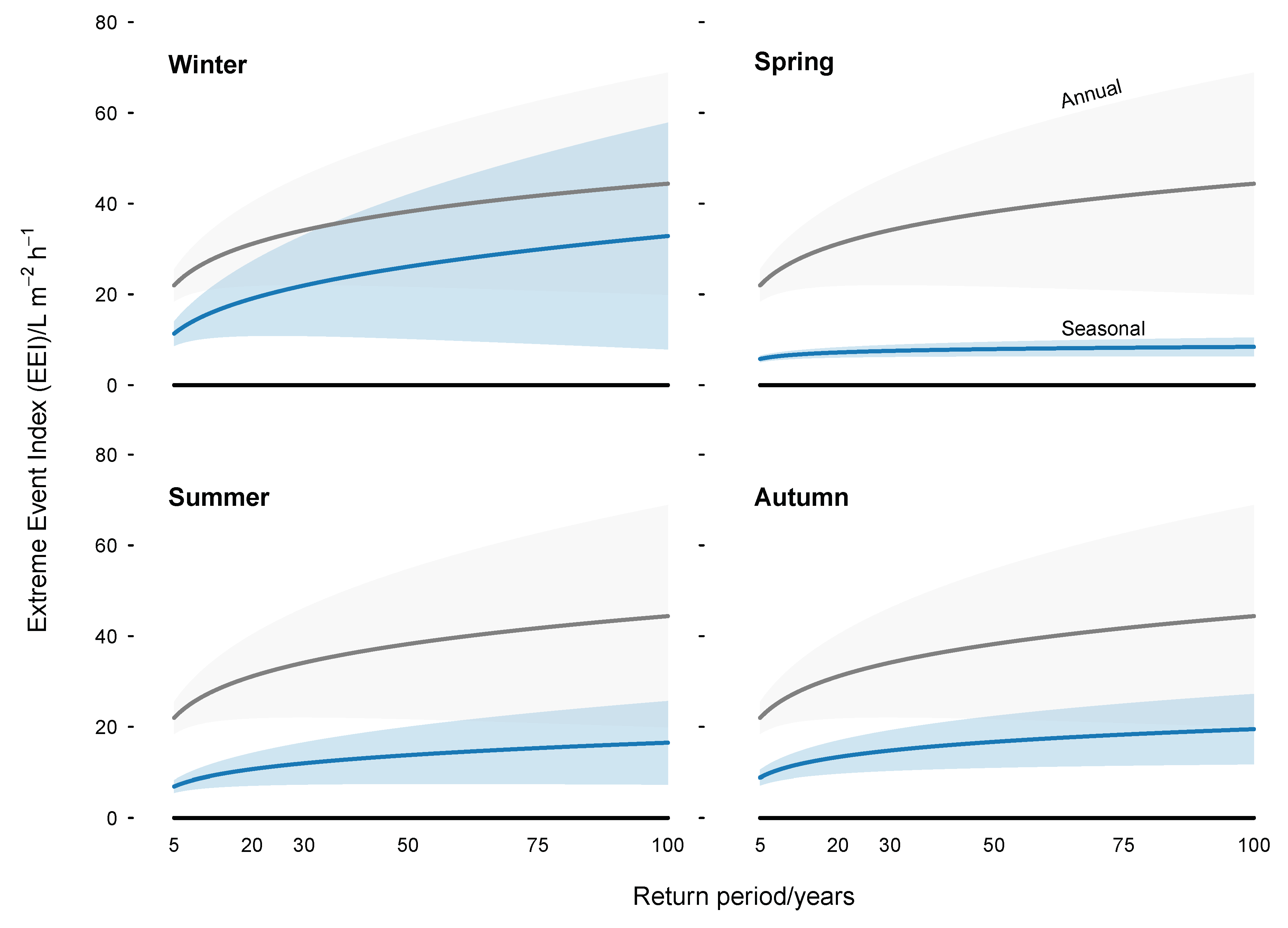
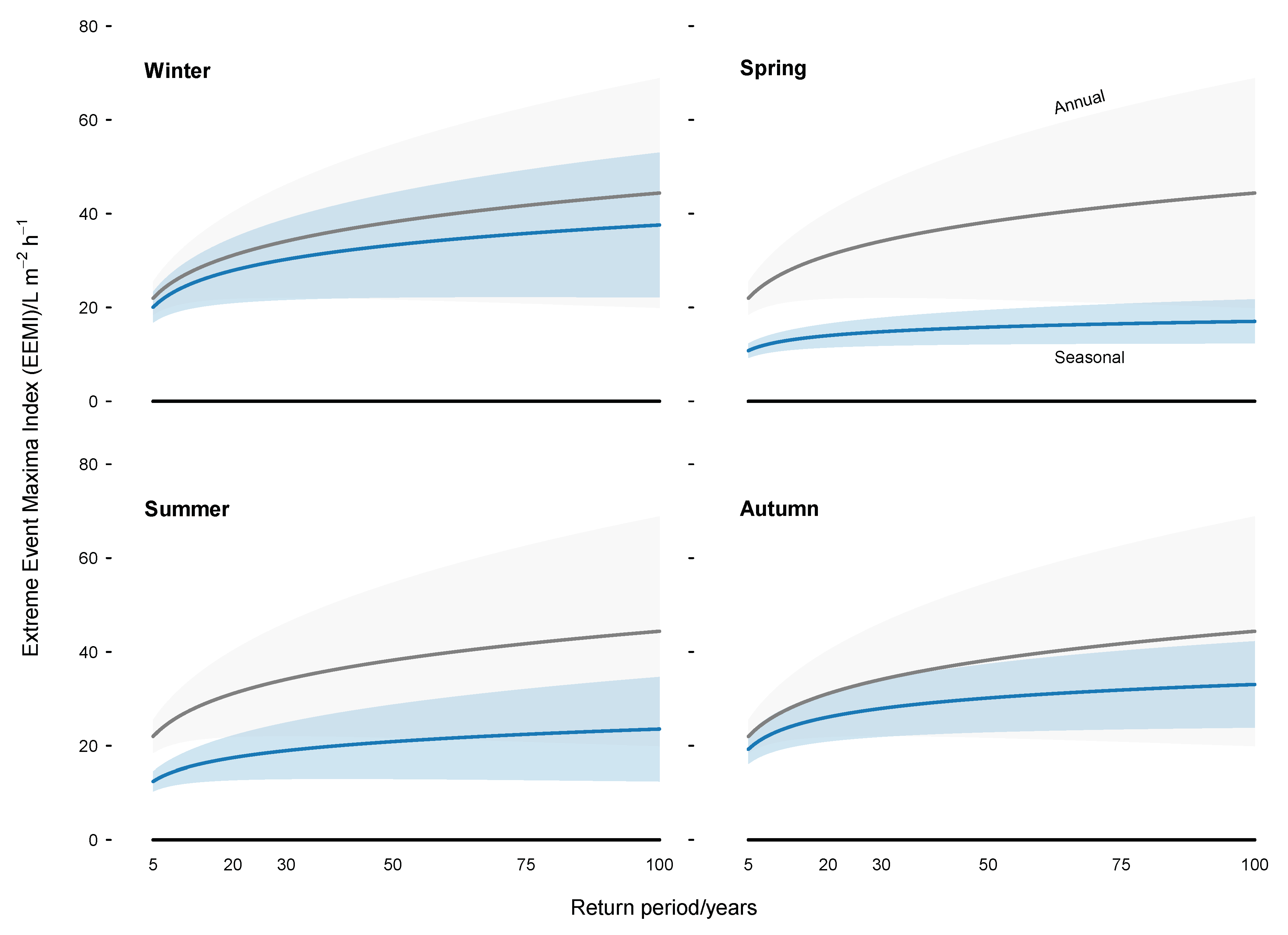
2.3.3. Seasonal Characteristics

Under the proposed time-binning rules for extreme events, an average of 353 events occur per year. These do not occur evenly over calendar seasons (

Table 1. Average annual frequency of wind-driven rain events derived from two time-binning rules for Plymouth, UK from 1986–2015.

Season	Proposed Time-Binning Rules	ISO15927-3 (Prolonged Exposure)
Winter (DJF)	113	4
Spring (MAM)	73	5
Summer (JJA)	71	5
Autumn (SON)	96	4
Total	353	18

). Previous work has demonstrated that climate change scenarios result in a polarising in the intensities of seasonal characteristics [15]. In Plymouth, UK, wind-driven rain events are most common during the autumn and winter months ($n=\{96,113\}$, respectively). In contrast, the spring and summer months experience fewer events ($n=\{73,71\}$, respectively).

In contrast, the time-binning rules for prolonged events produce an average of 18 events per year. These are more homogeneous across the year (varying by only one event between calendar seasons), and occur more frequently during the spring and summer months.

2.4. Intensity of Extreme Events

The Extreme Event Index (EEI) and Extreme Event Maxima Index (EEMI) can be determined for return periods of interest. They represent the average and maximum hourly wind-driven rain intensity, respectively, likely to occur once in the specified period.

2.4.1. GEV Fitting

The modelled Generalised Extreme Value (GEV) distribution reproduced the distribution of empirical annual indices. The modelled distributions were evaluated based on the quality of fit of the kernel densities of the annual indices (

Table 2. Squares of the Pearson correlation coefficient (R²) of the kernel densities for modelled GEV distributions compared to the empirical annual indices.

Season	Extreme Event Index (EEI)	Extreme Event Maxima Index (EEMI)
Winter (DJJ)	0.90	0.97
Spring (MAM)	0.98	0.99
Summer (JJA)	0.95	0.96
Autumn (SON)	0.91	0.99
Annual	0.89	0.93

). The GEV distributions for seasonal indices produce better fits than the annual indices. This is likely due to the seasonal variation of extreme event occurrence and intensity.

It is due to the manner in which the return periods are modelled that causes the annual EEI to be greater than that derived for any season. Since they are determined from the maxima that occurs in each year (or seasonal subset), the annual GEV distribution is fitted to a set of events that occur in varying seasons. Thus, the similarity between the winter and annual EEI suggests that most of the annual maxima occur in this season, but that they are otherwise also occurring in the spring and summer months.

2.4.2. Extreme Event Index (EEI)

The Extreme Event Index (EEI) is derived from the average hourly intensity for each event. It represents a generalised indication of the intensity of these events.

Figure 5 shows the EEI determined for the case study for four calendar seasons, which demonstrate varying characteristics. The winter and autumn months experience the highest and second-highest intensities, respectively, across the range of return periods. The spring months have the lowest intensities of extreme events. Despite the overall low intensities of WDR in Plymouth during summer months [15], the index demonstrates that extreme wind-driven rain events occur with intensities greater than those of the spring months.

Another important outcome is that separating the index by seasons increases the confidence interval. This is observed in Figure 5 by the relative sizes of the gray and blue areas across all seasons. Due to the duration of the input data (30 years), the 95% confidence interval for greater return periods increases significantly.

2.4.3. Extreme Event Maximum Index (EEMI)

The Extreme Event Maxima Index (EEMI) is derived from the maximum hourly intensity for each event (Figure 6). The EEMI is useful to evaluate particular impacts on buildings, such as the performance of rainwater goods. Similar to the EEI, the annual EEMI is greater than that of any season since the most extreme annual maxima occurs occurs within a mix of different seasons (see Section 2.4.2) for a more detailed explanation).

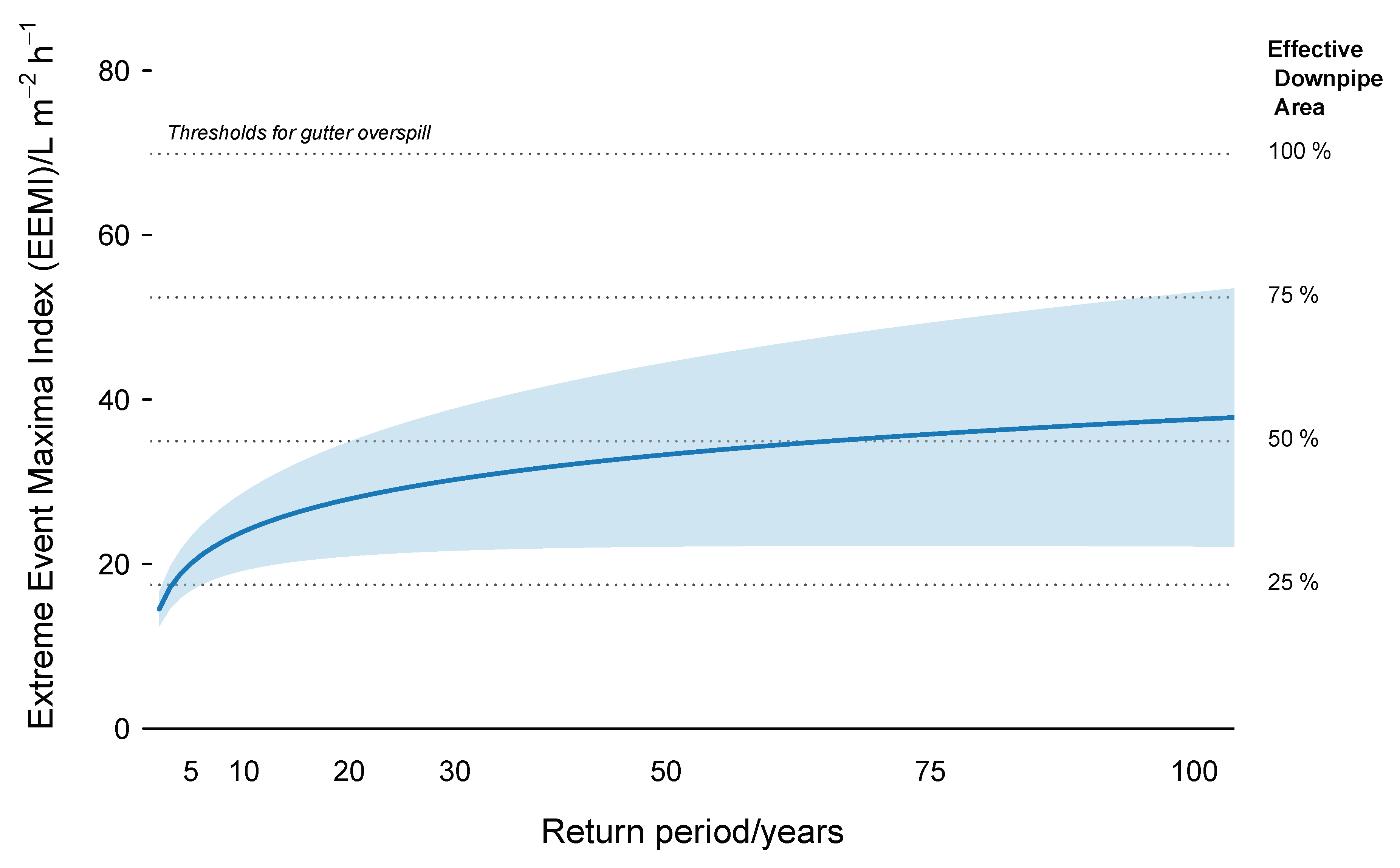
2.5. Threshold Assessment

The EEMI can be contextualised by how rainwater goods function on part of a historic structure oriented toward the southwest. The maximum hourly exposure represents the period of time during the event which poses the greatest risk of gutter overspill. This extends its use beyond a relative indicator of the intensity of exposure to an indicator of potential impact. To demonstrate this, a model of a gutter on a terraced house is used.

Figure 7 shows the same index for the winter calendar months as shown in a panel in Figure 6. The index is contextualised in a model of a standard gutter. The model demonstrates that, if the gutter is properly functioning, no extreme hourly exposure likely to occur once in a hundred years or less should cause the gutter to spill over. However, if the downpipe area is compromised (e.g., detritus blocks part of the drain area), the index falls within the range of possible extreme hourly intensities.

3. Discussion

3.1. Indices

3.1.1. Empirical Approaches to Wind-Driven Rain

A robust statistical risk index requires a long time series of data to accurately project infrequent events. This often limits the source of input to longitudinal meteorological measurements. Due to this, the wind-driven rain input is derived from empirical relationships, which have associated caveats [16]. However, if sufficient data exists or can be generated, the indices can be applied to measured and modelled wind-driven rain exposure. This would result in more accurate representations of the exposure to extreme weather events.

3.1.2. Urban Complexity

The indices can be further refined by applying factors to account for urban complexities and the influence they have on wind-driven rain exposure, e.g., those included in ISO 15927 [3]. Factors have been developed to account for, among others, topography, adjacent structures, as well as the position within a façade.

3.2. Seasonality

The case study demonstrated the importance of seasonal indicators. This acknowledges the varied seasonal characteristics observed in the northern hemisphere. In all cases, the indices derived for specific seasons were better modelled by the GEV distribution and had narrower confidence interval ranges. Thus, seasonal indices not only identify seasons which represent the greatest exposure to built heritage, but also increase the precision and accuracy of our predictions of their intensity.

3.3. Threshold Assessment

The threshold assessment for the EEMI demonstrates the potential for the EEMI to be used as a risk/impact indicator. This conversion was achieved by contextualising the wind-driven rain exposure within the performance of a gutter on a terraced building. This demonstrated the importance of gutter maintenance.

The threshold assessment undertaken for the case study likely underestimates the frequency of occurrence of gutter overspill. Standard meteorological measurement is reported hourly. However, several weather events (e.g., cloudbursts) often occur on shorter timescales. Since the exposure can only be assumed to occur over an hour (due to the data resolution), it may not represent the sub-hourly risk of gutter overspill. Two approaches could be taken to address this: (1) deriving the index from sub-hourly measurements, or (2) converting the hourly measured exposure into an equivalent exposure assuming a shorter time interval. In the latter, an hourly exposure could be assumed to have primarily occurred in a shorter period. Recent work [17] has shown that sub-hourly (10 min) return levels of extreme WDR events in the UK are frequently an order of magnitude greater than those recorded at 1 h intervals. Thus, the equivalent (hourly) EEMI would be the original multiplied by 10, or greater. If this approach is applied to the original EEMI presented in Figure 7, the threshold for gutter overspill (even with 100% effective downpipe area) is likely to be exceeded in any given 5-year period.

The threshold assessment is not intended to empirically generalise the potential impact for a general building in this location. It can be used for a specific building typology and context, or further adapted to account for other contextual factors (as discussed in Section 3.1.2). If the threshold assessment is applied to a building typology and context that is relevant to several regions and contexts, it can be used as a relative indicator of the potential impact.

3.4. Direct Exposure Assessment

Additional modifications to the EEI could be used to assess the direct exposure of building façades to wind-driven rain. A parameterisation for this would need to consider material properties and environmental conditions. This could be done with hygrothermal modelling [18] or controlled testing regimes.

3.5. Future Work and Outcomes

Maintenance of the urban heritage is highlighted in Historic England policy guidance as an important prerequisite to historic building protection with maintenance plans recommended for older buildings [19]. Despite the predominance in the urban landscape of the English-style terraced house, historic buildings are more varied in their construction. A significant component that could be further explored and developed in the model/index is the roof which can vary widely in materials and construction such as thatched, shingle, wood, concrete, metal or vinyl tiles or membrane with or without accompanying gutting. With the expected increase of extreme wind driven rain, how these materials will perform as an assembly with the external walls needs to modelled so that a typology of indices for different types of historic buildings can be developed.

4. Materials and Methods

4.1. Summary of Index Calculation Procedure

The determination of the proposed indices for extreme wind-driven rain events have several components:

• Determination of wind-driven rain exposure (herein semi-empirical).
• Time-binning procedure.
• Index selection.
• Extreme value analysis.
• Impact assessment.

4.2. Determination of Wind-Driven Rain Exposure

The intensity of wind-driven rain exposure was derived according to BS EN ISO 15927-3:2009 [3]. In accordance with the World Meteorological Organisation, statistical evaluations (and therefore indices) should be derived from 30 years or more of hourly data [20]. The semi-empirical relationship is a vector-based approach:

$$I=\frac{2}{9}v{r}^{\raisebox{1ex}{$8$}\!\left/ \!\raisebox{-1ex}{$9$}\right.}cos(D-\theta )$$

(1)

in which the hourly intensity of wind-driven rain, I as a volume per units area and time, is determined from vertical rainfall (i.e., precipitation), r, wind speed, v, the prevailing wind direction, D and the façade orientation $\theta$. The cosine component, despite its shortcomings [21], is used to represent the fractional exposure of a façade that is not directly impacted by the wind-driven rain. The parameters are typically meteorological measurements.

Several factors affect the accuracy of different aspects of the representation. This does not discount its use as a regional exposure index. The climate data may not accurately represent sub-hourly behaviour. For example, a drastic shift in the wind speeds mid-way through the hour may not be represented in the data, depending on how prevailing hourly wind speed has been recorded and calculated. Similarly, CFD modelling has shown that WDR exposure can vary significantly across a façade, primarily due to edge effects and sheltering [22]. For the purposes of this model, which represents WDR for exposure assessment on a fairly exposed roof system, these inaccuracies were deemed acceptable to demonstrate the proposed time-binning procedure. If greater accuracy is needed for a particular scenario or purpose, the index can instead be combined with measured and modelled wind-driven rain input.

4.3. Time-Binning

4.3.1. Existing Rules for Prolonged Exposure

The time-binning rules for prolonged exposure are taken from BS EN ISO 15927-3:2009 [3], requiring a break of ≥96 h between WDR events, selected to represent prolonged exposure of masonry façades. Caton experimentally demonstrated that up to 96 consecutive hours with no driving rain are necessary before evaporative losses exceed water ingress due to rain exposure [23]. In contrast to current standards, Caton distinguished between events by periods of 96 h without ‘appreciable’ driving rain, which was approximated as one tenth (10%) of the intensity for a statistical ‘once in three years’ event [23].

4.3.2. Proposed Rules for Extreme Events

The proposed time-binning rules are based on previous work by Lacy in which WDR events were determined from three rules based on measured data from the southwest England [24] (p. 101):

• The long event is deemed to be continuous if the aggregate of any breaks is not more than 10% of the whole.
• No single break is to be more than 5% of the time.
• The total duration is defined as the time from the beginning to the end of the event, including the dry breaks.

The rationale for these time-binning rules is to identify events (also commonly referred to as spells) with consistent exposure. Although it may appear that these rules produce events without regard for durations between events, these two approaches are statistically equivalent [25].

The time-binning was applied to the data series using a recursive function. A preliminary analysis applying these rules to measured data from a more exposed site in southwest England (see Section 2.1) determined that 99.7% of intervals between exposure, the proposed rules were equivalent to defining a WDR event as a period of consistent exposure without any hours of no wind-driven rain exposure. This provides a alternative approximation that is easier to calculate to apply the proposed time-binning rules to timeseries of exposure.

4.4. Index Selection

Before EVA can be applied, one of two indices is selected.

4.4.1. Extreme Event Index (EEI)

The Extreme Event Index (EEI) is derived from the average hourly intensity for each event. It represents a generalised indication of the intensity of these events.

4.4.2. Extreme Event Maximum Index (EEMI)

The Extreme Event Maxima Index (EEMI) is derived from the maximum hourly intensity for each event. The EEMI is useful to evaluate particular impacts on buildings, such as the performance of rainwater goods. In these scenarios, the maxima for each event represent the period of greatest risk. If the data resolution is greater than 1 h, it can be determined for sub-hourly intensities.

4.5. Extreme Value Analysis

Extreme value analysis (EVA) was applied to the time-binned wind-driven rain events. EVA is an established method in environmental applications [26] to evaluate behaviour near the extremes of probability distributions.

An ‘Annual Maxima Series (AMS)’ approach was taken, as identifying appropriate thresholds for the alternative “Peak Over Threshold” approach remains a subjective and contested challenge [27]. The AMS approach requires that the annual maxima of the data series (i.e., the most intense wind-driven event for each year) to be determined. A benefit of the AMS method is that the results are independent of the “population size” (number of events), i.e., comparisons can be made between sites and periods of time that experience different numbers of events. The AMS is fit to the Generalised Extreme Value (GEV) continuous probability distribution:

$$F\left(x\right)=e^{-(1-{(\xi \frac{x-\mu }{\sigma })}^{\raisebox{1ex}{$1$}\!\left/ \!\raisebox{-1ex}{$\xi $}\right.}}$$

(2)

Three parameters determine the characteristics of the distribution. The location parameter, $\mu$, describes the horizontal shift, while the scale parameter, $\sigma$, and the shape parameter, $\xi$, describe the spread and behaviour at the tails of the distribution, respectively. The shape parameter is derived from skewness, as it represents where the majority of the data lie, which creates the tails of the distribution [28].

The Gumbel distribution has previously been employed to describe wind-driven events [5,14], which can be considered a special case of the GEV in which $\xi =0$. Distributions with two parameters (such as the Gumbel) have smaller standard error, but larger bias than three-parameter distributions, especially for small sample sizes [29].

After fitting the distribution parameters, the EVA is combined with the concept of return periods, which estimate the likelihood of an event (or statistically ‘expected frequency’). The intensity, $Q_n$ of the most extreme wind-driven rain event expected every n years is determined from:

$$Q_n=\mu +\frac{\sigma }{\xi }\left\{1-\left(-log{\left(\frac{n-1}{n}\right)}^{\xi }\right)\right\}$$

(3)

The index can be determined for sub-annual periods. Previous work [15] has demonstrated that climate change scenarios are predicted to result in increasingly polarised seasonal behaviour for wind-driven rain exposure. Thus, assessment of wind-driven rain exposure and impact should consider these trends in determining indices. While this is paramount for comparative studies under climate change regimes, presenting historical and contemporary exposure using seasonal indices facilitates comparison, for ease of calculation, it is worth noting that the EEMI can be derived from the annual/season AMS derived from the hourly maximum, without applying the time-binning procedure. These values are equivalent.

4.6. Impact Assessment

A mass balance model was developed to represent the response of rainwater goods (a gutter system) to wind-driven rain events. On the basis of the following equations (Equations (4)–(7)), which refer to the rainwater goods associated with a single building façade, the quantity of overspill within the gutter (the ‘system’) is determined as a function of the rainfall intensity. The balance equation for mass (Equation (4)) is presented as a volume balance, since the system consists of only one component with constant density. It consists of three terms:

$${\dot{V}}_{\mathrm{acc}}={\dot{V}}_{\mathrm{in}}-{\dot{V}}_{\mathrm{out}}$$

(4)

relating the rate accumulated volume of water, ${\dot{V}}_{\mathrm{acc}}$, to the net balance of the volume into the gutter system and that which exits it, ${\dot{V}}_{\mathrm{in}}$ and ${\dot{V}}_{\mathrm{out}}$, respectively. The model is integrated over a single time step, as the timescales of dynamic components (e.g., rainwater flowing down the roof surface, travelling through the gutter) are much shorter than the time resolution of the input data (1 h). The same would be true for data at relatively-high time resolutions for meteorological measurement, e.g., 5 min.

The rate of volume entering the system is represented by the volume of wind-driven rain exposure that impacts the roof system and the exposed gutter in a given time period. This is determined by multiplying the specific rate of wind-driven rain, $\dot{r}$, with the surface areas of the roof ($A_r$) and gutter ($A_g$):

$${\dot{V}}_{\mathrm{in}}=\dot{r}\times F_R(A_r+A_g)\times C$$

(5)

in which C is a runoff coefficient (taken as 1 unless under special circumstances) and $F_R$ is a risk factor. The risk factor for eaves gutters is taken to be 1. However, BS 12056-3 suggests a risk factor of 3.0 should be applied for non-eaves gutters for “buildings where an exceptional degree of protection is necessary, e.g., buildings housing outstanding works of art.” [30] (p. 9). We argue this risk factor should be used for built heritage if the edifices are considered to be works of art in their own right, i.e., having artistic/aesthetic/architectural value [31].

The rate of volume exiting the system is primarily dependent on the dimensions of the downpipe. For a round downpipe connected to a rectangular gutter, the flow rate is represented by [30]:

$${\dot{V}}_{\mathrm{out}}=\frac{k_{\mathrm{o}}D{h}^{1.5}}{7500}$$

(6)

in which ${\dot{V}}_{\mathrm{out}}$ has units of L s⁻¹, while all other measurements are in units of mm. This represents Wier flow (when $h=D/2$) when there is a gap of at least 5% of the diameter of the outlet. The diameter of the downpipe is twice that of the radius, $r_d$ = $0.5·D$. The outlet coefficient, $k_{\mathrm{o}}$, dimensionless, is taken as 1.0 for unobstructed outlets, and 0.5 for outlets fitted with strainers or gratings. The head at outlet, h, is represented by a determined factor $F_{\mathrm{h}}$ = 0.47 [30] multiplied by the maximum flow height (taken here to be the gutter height, $h_g$). This volumetric flow rate is multiplied by the process duration to determine the total flow rate.

A dimensionless parameter is introduced to represent the effective area of the downpipe, f. This factor, ranging from 0 to 1, represents the effect of blockage which can result from of maintenance. It is applied to the volumetric outflow rate.

The volume of a rectangular gutter is represented by $V_g=l_g{w}_g{d}_g$, which represents the maximum volume of water it can hold as a function the length, height, and width of the gutter, respectively. This was further simplified by assuming a square cross-sectional area to $V_g=l_g{\left(d_g\right)}^2$. Thus, a gutter is modelled to overspill when the accumulated volume of water, $V_{\mathrm{acc}}={\dot{V}}_{\mathrm{acc}}\Delta t$, satisfies the condition:

$$V_{\mathrm{acc}}>V_g$$

(7)

Parameter selection was derived from a combination of standards and informal observation (

Table 3. Parameters for the overspill model, with affiliated source and units, where appropriate.

Parameter	Source	Value
Width of roof, $w_r$ = length of gutter, $l_g$	informal observation	5 m
Length of roof (eave to crest), $l_r$	informal observation	5 m
Area of roof (eave to crest), $A_r=w_g\times l_r$	Calculated	25 m2
Depth of gutter, $d_g$	BS EN 8530:2010 [32]	68.8 mm
Surface area of gutter, $A_g=d_g\times l_r$	Calculated	0.344 m2
Radius of downpipe, $r_d$	BS EN 8530:2010 [32]	0.0602 m
effective gutter area coefficient, f	-	1, unless otherwise stated
downpipe coefficient, $k_{\mathrm{o}}$	with strainer	0.5
downpipe head, h	BS EN 12056–3:2000 [30]	$0.47·d_g$ mm
Rate of wind-driven rain, $\dot{r}$	measured climate data, ISO 15927–3:2009 [3]	dependent on return period, L h−1

). For the purposes of this paper, the required accuracy for parameters is low, as it attempts to represent a common physical configuration. Each parameter could be adapted to suit a specific scenario, heritage typologies, or built context.

References

1. Cassar, M.; Hawkings, C. Engineering Historic Futures Stakeholders Dissemination and Scientific Research Report. 2007. Available online: https://discovery.ucl.ac.uk/id/eprint/2612/1/2612.pdf (accessed on 2 January 2020).
2. BSI. BS 8104:1992—Code of Practice for Assessing Exposure of Walls To Wind-Driven Rain; Standard, British Standards Institution: London, UK, 1992. [Google Scholar]
3. ISO. BS en ISO 15927-3: 2009: Hygrothermal Performance of Buildings— Calculation and Presentation of Climatic Data—Part 3: Calculation of A Driving Rain Index for Vertical Surfaces From Hourly Wind and Rain Data; Standard, International Standards Organisation: London, UK, 2009. [Google Scholar]
4. Kinnison, R.R. Applied Extreme Value Statistics; Battelle Press: Columbus, OH, USA, 1985. [Google Scholar]
5. Pérez-Bella, J.M.; Domínguez-Hernández, J.; Rodríguez-Soria, B.; del Coz-Díaz, J.J.; Cano-Suñén, E. Combined use of wind-driven rain and wind pressure to define water penetration risk into building façades: The Spanish case. Build. Environ. 2013, 64, 46–56. [Google Scholar] [CrossRef]
6. Sabbioni, C.; Brimblecombe, P.; Cassar, M. The Atlas of Climate Change Impact on European Cultural Heritage: Scientific Analysis and Management Strategies; Anthem Press: London, UK, 19 Number 2010. [Google Scholar]
7. Winkler, E.M. Important agents of weathering for building and monumental stone. Eng. Geol. 1966, 1, 381–400. [Google Scholar] [CrossRef]
8. Stephenson, V.; D’Ayala, D. Structural Response of Masonry Infilled Timber Frames to Flood and Wind Driven Rain Exposure. J. Perform. Constr. Facil. 2019, 33, 04019028. [Google Scholar] [CrossRef]
9. D’Ayala, D.; Aktas, Y.D. Moisture dynamics in the masonry fabric of historic buildings subjected to wind-driven rain and flooding. Build. Environ. 2016, 104, 208–220. [Google Scholar] [CrossRef] [Green Version]
10. UK Met Office. MIDAS: UK Hourly Weather Observation Data; UK Met Office: Exeter, UK, 2006. [Google Scholar]
11. UK Met Office. MIDAS: UK Hourly Rainfall Data; UK Met Office: Exeter, UK, 2006. [Google Scholar]
12. Gould, J. Architecture and the plan for Plymouth: The legacy of a British city. Archit. Rev. 2007, 221, 78–83. [Google Scholar]
13. Strong Winds: Woman Killed and Ferry Travel Disrupted. BBC News. 2 November 2019. Available online: https://www.bbc.co.uk/news/uk-england-50273590 (accessed on 7 November 2019).
14. Orr, S.A.; Viles, H. Characterisation of building exposure to wind-driven rain in the UK and evaluation of current standards. J. Wind Eng. Ind. Aerodyn. 2018, 180, 88–97. [Google Scholar] [CrossRef]
15. Orr, S.A.; Young, M.; Stelfox, D.; Curran, J.; Viles, H. Wind-driven rain and future risk to built heritage in the United Kingdom: Novel metrics for characterising rain spells. Sci. Total Environ. 2018, 640, 1098–1111. [Google Scholar] [CrossRef] [PubMed]
16. Blocken, B.; Carmeliet, J. A review of wind-driven rain research in building science. J. Wind Eng. Ind. Aerodyn. 2004, 92, 1079–1130. [Google Scholar] [CrossRef]
17. Chan, S.; Kendon, E.; Roberts, N.; Fowler, H.; Blenkinsop, S. The characteristics of summer sub-hourly rainfall over the southern UK in a high-resolution convective permitting model. Environ. Res. Lett. 2016, 11, 094024. [Google Scholar] [CrossRef]
18. Hansen, T.K.; Bjarløv, S.P.; Peuhkuri, R. The effects of wind-driven rain on the hygrothermal conditions behind wooden beam ends and at the interfaces between internal insulation and existing solid masonry. Energy Build. 2019, 196, 255–268. [Google Scholar] [CrossRef]
19. Historic England. Maintenance Plans for Older Buildings. Available online: https://historicengland.org.uk/advice/technical-advice/buildings/maintenance-plans-for-older-buildings/ (accessed on 12 December 2019).
20. Guttman, N. Guide to Climatological Practices; Technical Report 100; World Meteorological Organisation: Geneva, Switzerland, 2011. [Google Scholar]
21. Blocken, B.; Carmeliet, J. On the validity of the cosine projection in wind-driven rain calculations on buildings. Build. Environ. 2006, 41, 1182–1189. [Google Scholar] [CrossRef]
22. Blocken, B.; Carmeliet, J. Validation of CFD simulations of wind-driven rain on a low-rise building facade. Build. Environ. 2007, 42, 2530–2548. [Google Scholar] [CrossRef]
23. Prior, J. Directional Driving Rain Indices for the United Kingdom: Computation and Mapping (Background to BSI Draft for Development DD93); Building Research Establishment: Glasgow, UK, 1985. [Google Scholar]
24. Lacy, R. Climate and Building in Britain; Her Majesty’s Station Office (HMSO): Richmond, UK, 1977. [Google Scholar]
25. Ignaccolo, M.; Michele, C.D. A non arbitrary definition of rain event: The case of stratiform rain. arXiv 2009, arXiv:0911.3941. [Google Scholar]
26. Finkenstadt, B.; Rootzén, H. Extreme Values in Finance, Telecommunications, and The Environment; CRC Press: Boca Raton, FL, USA, 2003. [Google Scholar]
27. Solari, S.; Losada, M. A unified statistical model for hydrological variables including the selection of threshold for the peak over threshold method. Water Resour. Res. 2012, 48. [Google Scholar] [CrossRef]
28. Millington, N.; Das, S.; Simonovic, S.P. The Comparison of GEV, Log-Pearson Type 3 and Gumbel Distributions In the Upper Thames River Watershed Under Global Climate Models; Technical Report 77; Department of Civil and Environmental Engineering, The University of Western Ontario: London, UK, 2011. [Google Scholar]
29. Cunnane, C. Statistical Distributions for Flood Frequency Analysis. Technical Report. 1989. Available online: http://agris.fao.org/agris-search/search.do?recordID=XF9090879 (accessed on 2 January 2020).
30. BS. BS en 15927–2: Gravity Drainage Systems Inside Buildings. Sanitary Pipework, Layout and Calculation; Standard, British Standards Institute: London, UK, 2000. [Google Scholar]
31. Martínez, A.H. Conservation and restoration in built heritage: A western European perspective. In The Ashgate Research Companion to Heritage and Identity; Ashgate Publishing, Ltd.: Farnham, UK, 2008; pp. 245–263. [Google Scholar]
32. BSI. BS 8530:2010—Traditional-Style Half Round, Beaded Half Round, Victorian Ogee and Moulded Ogee Aluminium Rainwater Systems. Specification; Standard, British Standards Institution: London, UK, 2010. [Google Scholar]
Figure 1. Wind-driven rain intensity during January 2015 in Plymouth, UK. The black bar represents the total exposure during each event under the proposed time-binning rules, while the horizontal white line shows the maximum exposure in a single hour. Under the ISO 15927-3 time-binning rules, the entire month is a single wind-driven rain event. This does not represent the several extreme short exposures that occurred during that period. The thickness of the line is a measure of the duration of the event.
Atmosphere 11 00163 g001
Figure 2. Boxplots of wind-driven rain intensities and average intensities derived from two time-binning rules during 1986–2015 for Plymouth, UK.
Atmosphere 11 00163 g002
Figure 3. Boxplots of the maximum wind-driven rain intensities derived from the proposed time-binning rules for an extreme event index between 1986–2015 in Plymouth, UK.
Atmosphere 11 00163 g003
Figure 4. A plot of the fraction of hours in which there was active rain for events time binned according to the ISO 15927-3 [3] rules for prolonged exposure.
Atmosphere 11 00163 g004
Figure 5. The Extreme Event Index (EEI) for calendar seasons based on semi-empirical wind-driven rain exposure in Plymouth UK between 1986 and 2015. Shaded areas represent 95% confidence intervals.
Atmosphere 11 00163 g005
Figure 6. The Extreme Event Maxima Index (EEMI) for calendar seasons based on semi-empirical wind-driven rain exposure in Plymouth UK between 1986 and 2015. Shaded areas represent 95% confidence intervals.
Atmosphere 11 00163 g006
Figure 7. The Extreme Event Maxima Index (EEMI) for the winter calendar season based on semi-empirical wind-driven rain exposure in Plymouth UK between 1986–2015. Shaded areas represent 95% confidence intervals for the return period modelling. The return levels (the EEMI for different return periods) are contextualised within a model of a gutter managing rainshed on a terraced house. The threshold for gutter overspill are determined by several localised factors, including topography, geometry, and context, which would impact the confidence intervals if adapted to reflect other scenarios than the one studied herein.
Atmosphere 11 00163 g007