Article

Source Apportionment of Fine Organic and Inorganic Atmospheric Aerosol in an Urban Background Area in Greece

by
Manousos Ioannis Manousakas
1,*,
Kalliopi Florou
1 and
Spyros N. Pandis
1,2,3
1
Institute of Chemical Engineering Sciences, (FORTH/ICE-HT), 26504 Patras, Greece
2
Department of Chemical Engineering, University of Patras, 26504 Patras, Greece
3
Department of Chemical Engineering, Carnegie Mellon University, Pittsburgh, PA 15213, USA
*
Author to whom correspondence should be addressed.
Atmosphere 2020, 11(4), 330; https://doi.org/10.3390/atmos11040330
Submission received: 7 March 2020 / Revised: 25 March 2020 / Accepted: 26 March 2020 / Published: 29 March 2020
(This article belongs to the Special Issue Sources and Composition of Ambient Particulate Matter)

Abstract

:
Fine particulate matter (PM) originates from various emission sources and physicochemical processes. Quantification of the sources of PM is an important step during the planning of efficient mitigation strategies and the investigation of the potential risks to human health. Usually, source apportionment studies focus either on the organic or on the inorganic fraction of PM. In this study that took place in Patras, Greece, we address both PM fractions by combining measurements from a range of on- and off-line techniques, including elemental composition, organic and elemental carbon (OC and EC) measurements, and high-resolution Aerosol Mass Spectrometry (AMS) from different techniques. Six fine PM2.5 sources were identified based on the off-line measurements: secondary sulfate (34%), biomass burning (15%), exhaust traffic emissions (13%), nonexhaust traffic emissions (12%), mineral dust (10%), and sea salt (5%). The analysis of the AMS spectra quantified five factors: two oxygenated organic aerosols (OOA) factors (an OOA and a marine-related OOA, 52% of the total organic aerosols (OA)), cooking OA (COA, 11%) and two biomass burning OA (BBOA-I and BBOA-II, 37% in total) factors. The results of the two methods were synthesized, showcasing the complementarity of the two methodologies for fine PM source identification. The synthesis suggests that the contribution of biomass burning is quite robust, but that the exhaust traffic emissions are not due to local sources and may also include secondary OA from other sources.

1. Introduction

Atmospheric particulate matter (PM) has serious adverse effects on human health and the environment [1,2,3,4]. PM originates from various emission sources but is also the product of gas-to-particle processes in the atmosphere (secondary PM). The identification of the different types of PM sources and the quantification of their contributions, including the role of natural and anthropogenic sources, is a critical step in our efforts to reduce the PM effects on human health [5]. The process of identifying PM sources is called source apportionment and there is a wide range of methods that have been proposed based on the available measurements [6]. A widely used source apportionment approach is the use of various types of source-receptor models [7,8,9,10,11]. Most receptor models are based on the assumption that at the receptor site, the time dependence of the concentration of PM components originating from the same source will be the same. The concentrations of the relevant PM chemical components are measured in a large number of samples gathered at the receptor site over time. Components with similar temporal variability are grouped together in a minimum number of factors that explain the variability of the complete dataset. It is assumed that each factor is associated with a source or source type. Those factors can be considered as the chemical fingerprint of the PM sources and lead to their identification. Positive Matrix Factorization (PMF) is one of the most useful source-receptor analysis approaches [12]. PMF introduces a weighting scheme taking into account errors of the individual measurements. Adjustment of the corresponding error estimates also allows it to handle missing and below detection limit data. One of its major advantages compared to other approaches is that it obtains only factors with positive elements using appropriate constraints.
Usually, source-apportionment studies focus either on the organic [13,14] or on the inorganic components of PM [15,16]. To fully assess the particulate related pollution in an area, it is important to examine the sources of both the organic and the inorganic fraction of PM. In the current study that took place in Patras, Greece, we focus on both the sources of organic and inorganic fractions using appropriate measurement techniques.
Greece is located in the Eastern Mediterranean, which is characterized as an air pollution hotspot located at the crossroad of air masses coming from Asia, Europe, and Africa [17]. Forest fires and agricultural burning emissions affect the area during the dry season, while the high radiation intensity all year long and the relatively high temperatures enhance the formation of secondary PM. Patras is a medium-sized city located in the northwest Peloponnese. Previous studies have shown that PM1 in the area is composed mainly of OA (organic aerosols) 45% and sulfate 38% [18,19]. Transportation, biomass burning (residential and agricultural), and shipping emissions have been found to be major local sources in the past [8,20], but long-range transport is an important source, especially during the summer, spring, and fall. Almost all of the sulfates and 40–90%, depending on the season, of the organic aerosol are believed to be transported to the city from other areas [21]. However, the situation in Patras and the rest of Greece has changed significantly during the last few years due to the financial crisis. This has led to an apparent reduction of the emissions of some sources (transportation, industry), but also to the increase of others (residential biomass burning). Organic aerosol (OA) and especially residential wood burning, have dramatically increased due to the Greek financial crisis [22]. A 30% increase in the PM2.5 mass concentration as well as a 2−5 fold increase in the concentration of wood smoke tracers, including potassium, levoglucosan, mannosan, and galactosan has been reported for the city of Thessaloniki [23], while the concentrations of fuel oil tracers (e.g., Ni and V), have declined by 20−30%. One of the goals of the present study is to try to quantify these changes using recent measurements and improved source-apportionment techniques.

2. Experiments

2.1. Experimental Design

The sampling site was located in a suburban area, around 7 km northeast of the city center (38°18′ N, 21°47′ E) in the Institute of Chemical Engineering Sciences (FORTH/ICE-HT) and at an elevation of 85 m above sea level. The sampling station is surrounded by olive trees, while the coast is approximately 3 km away. The closest major road is found at a distance of 1 km. Sampling took place from late October until the start of November 2018 and late February to June 2019.
The size-resolved chemical composition of the submicrometer aerosol (organics, nitrate, sulfate, chloride, and ammonium) was monitored using a High-Resolution Time-of-Flight Aerosol Mass Spectrometer (HR–ToF–AMS) from Aerodyne [24]. The sampled aerosol during this study was not dried, while the vaporizer surface temperature was set at 600 °C. The HR–ToF–AMS measurements were collected with a 3 min temporal resolution. The software toolkit SQUIRREL v1.57I (Sueper, D, ToF-AMS Data Analysis Software) in Igor Pro (Wavemetrics) was used for all the HR–ToF–AMS data analysis combined with the Peak Integration by Key Analysis (PIKA v1.16I package) (Sueper, D, ToF-AMS Data Analysis Software) software. For the calculation of the elemental ratios measured by the HR–AMS, the improved ambient approach was used [25].
A Super Speciation Air Sampling System Sampler (Met One SuperSASS) operating at a flow rate of 6.7 L min−1 was used to collect PM2.5 samples every 24 h, both on PTFE (Whatman, PTFE, White Plain, 0.2 μm × 47 mm) and on quartz (Pall 2500 QAO-UP 47 mm) filters The Super SASS sampler is based on designs that have been field tested for several years in the US; eight years with three years of testing in the EPA program. These filters were used for the measurement of the daily average PM2.5 mass concentration and its chemical composition. The PM2.5 mass concentration of each filter collected was determined by gravimetric analysis using a six-digit microbalance at 35% relative humidity (RH). Both sampling and gravimetric analysis were compliant with US EPA requirements. The PM2.5 mass concentration measured at 35% relative humidity includes less water than measurements at higher RH values.
The concentrations of organic carbon (OC) and elemental carbon (EC) were measured by thermo-optical transmittance (TOT) analysis (Lab OC-EC Aerosol Analyzer, Sunset Laboratory, Inc., Tigard, Washington, DC, USA) [26]. Quartz filter samples were heated first up to 650 °C in He and then up to 850 °C in a mixture of 2% O2 in He, using the controlled heating ramps of the EUSAAR2 thermal protocol [27]. OC evolved in the inert atmosphere, while EC was oxidized in the He–O2 atmosphere. A charring correction was applied by monitoring the sample transmittance throughout the heating process. The limit of detection for the TOT analysis is 0.2 μg cm−2. Before sampling, the quartz fiber filters were pretreated at 500 °C for 6 h to remove possible organic contaminants. Laboratory and field blanks were collected and analyzed following the same procedures as those adopted for the samples. The QA/QC procedures described in EN 16,909:2017 were followed during the OC/EC analysis.
A high energy, polarization geometry energy-dispersive XRF spectrometer (Epsilon 5 by PANalytical, Almelo, the Netherlands) was used for the elemental analysis of PM2.5 samples. Epsilon 5 is constructed with optimized Cartesian-triaxial geometry composed of several secondary targets for attaining lower spectral background and with extended K line excitation allowing it to operate the X-ray tube at a high voltage of 100 kV. The secondary target-XRF spectrometer includes a side-window low power X-ray tube with a W/Sc anode (spot size 1.8–2.1 cm, 100 kV maximum voltage, 6 mA current, 600 W maximum power consumption). A Ge X-ray detector detects the characteristic X-rays emitted from the sample with 140 eV FWHM at MnKα, 30 mm2, and 5-mm thick Ge crystal with an 8 μm Be window. The spectrometer used is equipped with eight secondary targets (Al, CaF2, Fe, Ge, Zr, Mo, Al2O3, KBr, and LaB6) that can polarize the X-ray tube-generated incident radiation through Barkla scattering. The methodology that was used for the elemental composition analysis is described in detail elsewhere [8]. The 20 elements determined by the ED–XRF method were Na, Mg, Al, Si, S, Cl, K, Ca, Ti, V, Cr, Mn, Fe, Co, Ni, Cu, Zn, Br, Sr, and Pb.
In total, 55 PM2.5 samples were collected for each filter type (Teflon and quartz). The sampling campaign took place during five periods, October–November 2018 (12 samples), February–March 2019 (13 samples), April 2019 (10 samples), May 2019 (10 samples), and June 2019 (10 samples).
The AMS measurements cover the PM1 range while the filter samples and the corresponding analysis were in the PM2.5 range. This small discrepancy in size ranges was unavoidable because of the characteristics of the AMS used in this study. The AMS measurements are mainly used in this study for the organic aerosol characterization and source apportionment. Given that most of the organic aerosol in the PM2.5 is in submicrometer particles, this size discrepancy does not affect our conclusions and the synthesis of the results from the two types of measurements.

2.2. PMF Analysis

The basic equation for the solution of the mass balance problem is common for all the utilized multivariate receptor models, including PMF:
X i j = k = 1 p g i k f k j + e i j
where Xij is the concentration of species j measured on sample i, p is the number of factors contributing to the measured PM, fkj is the concentration of species j in factor profile k, gik is the relative contribution of factor k to sample i, and eij is error of the PMF model for the jth species measured in sample i. The values of gik and fkj are adjusted until a minimum value of Q for a given p is found where Q is defined as:
Q = j = 1 m i = 1 n e i j 2 s i j 2
where sij is the uncertainty of the jth species concentration in sample i, n is the number of samples, and m is the number of species. Additional terms are added to the Q term in Equation (2) to make sure that only non-negative solutions are obtained.

2.3. Trajectory Analysis and Long-Range Transport

To identify the origin of the various aerosol components, air mass back-trajectories arriving at the site were analyzed by statistical methods. For the analysis of the back trajectories, the OPENAIR package was used [28]. The trajectories were calculated using the National Oceanic and Atmospheric Administration (NOAA) HYSPLIT 4.0 model [29,30].
In this study, 120 h (5 days) backward air mass trajectories arriving at the sampling site were computed. Global data assimilation system (GDAS) meteorological files were used as inputs for the backward trajectory computation. The backward trajectories were computed every three hours (ending at 00:00, 03:00, 06:00, 09:00, 12:00, 15:00, 18:00, and 00:00 UTC) for each day of the period of study at 500 m above ground level. The measured concentration of the PM component during the sampling period was assigned to all trajectories during that period.
To identify the possible position of sources that are affecting the concentration of PM chemical components measured, the Potential Source Contribution Function (PSCF) [31] was calculated. The PSCF is calculated as:
PSCF = m i j n i j
where nij is the number of times that the trajectories passed through the cell (i, j) and mij is the number of times that a source concentration was high when the trajectories passed through the cell (i, j). The criterion for determining mij is based on the distribution of the measured values (e.g., upper quartile).

3. Results

3.1. PM2.5 Chemical Composition

The average PM2.5 concentration measured was 12.4 ± 6.4 μg m−3 (Table 1). The highest average concentration was observed during October–November 2018 (14.8 μg m−3) followed by March 2019 (14.3 μg m−3). The lowest PM2.5 concentrations were recorded during April and May 2019, with average concentrations of 8.3 and 9.5 μg m−3, respectively.
The average OC and EC concentrations were 2.85 and 0.38 μg m−3. To calculate OA from OC concentration, the PM1 OA/OC was determined based on the AMS measurements and found to be equal to 2.25. This ratio was then used for the conversion of the PM2.5 OC to OA. The OA represented on average 52% of the PM2.5 concentration with the EC contributing another 3%. When compared to results from other Greek cities, these concentrations are comparable to the ones reported for the Athens suburbs [26] and lower than those reported for urban and traffic sites in Athens and Thessaloniki [26,32,33]. Recent studies conducted in another European city, Lisbon, Portugal, have also reported higher concentrations of OC and EC (4.02 and 6.61 μg m−3 respectively) [34]. The highest average OC concentrations were recorded during November 2018 (3.77 μg m−3) and March 2019 (4.19 μg m−3). These two months also had the highest EC levels with averages of 0.6 and 0.59 μg m−3, respectively. The average OC/EC ratio was 7.5, suggesting relatively low contribution from traffic emissions [26]. In general, the OC/EC ratio values reported for other European cities show OC/EC ratios of less than 2 at curbside sites, 2–9 at urban background sites, and increase with decreasing fresh anthropogenic emissions, reaching values above 10 at rural sites [33,35].
Fifteen elements had concentrations consistently higher than the detection limit (Table 1). Sulfur had the highest average concentration at 0.92 μg m−3. Assuming that all was in the form of sulfate, it represented 22.2% of the PM2.5. Silicon, sodium, aluminum, potassium, chloride, calcium, and iron also had relatively high average concentrations.

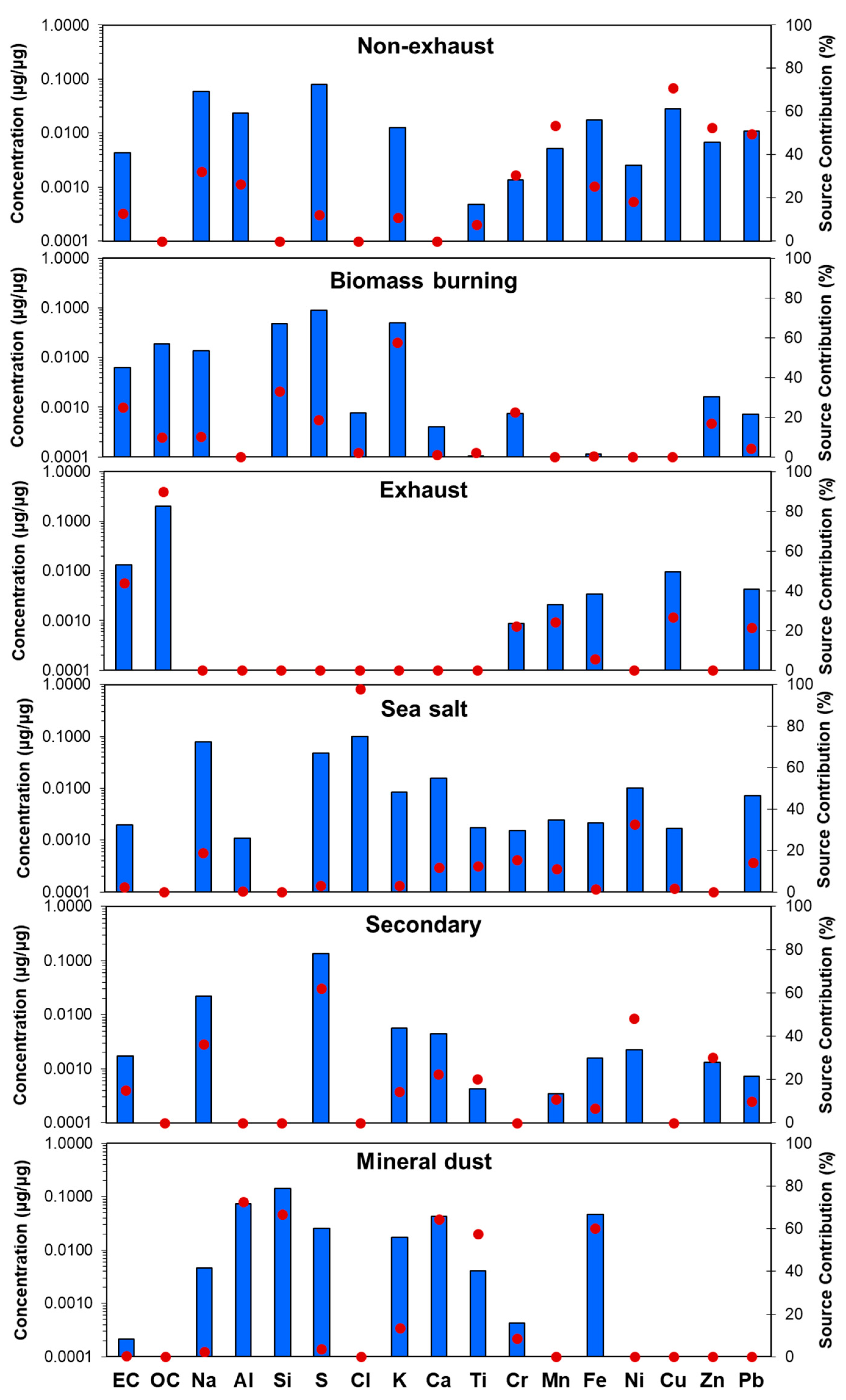
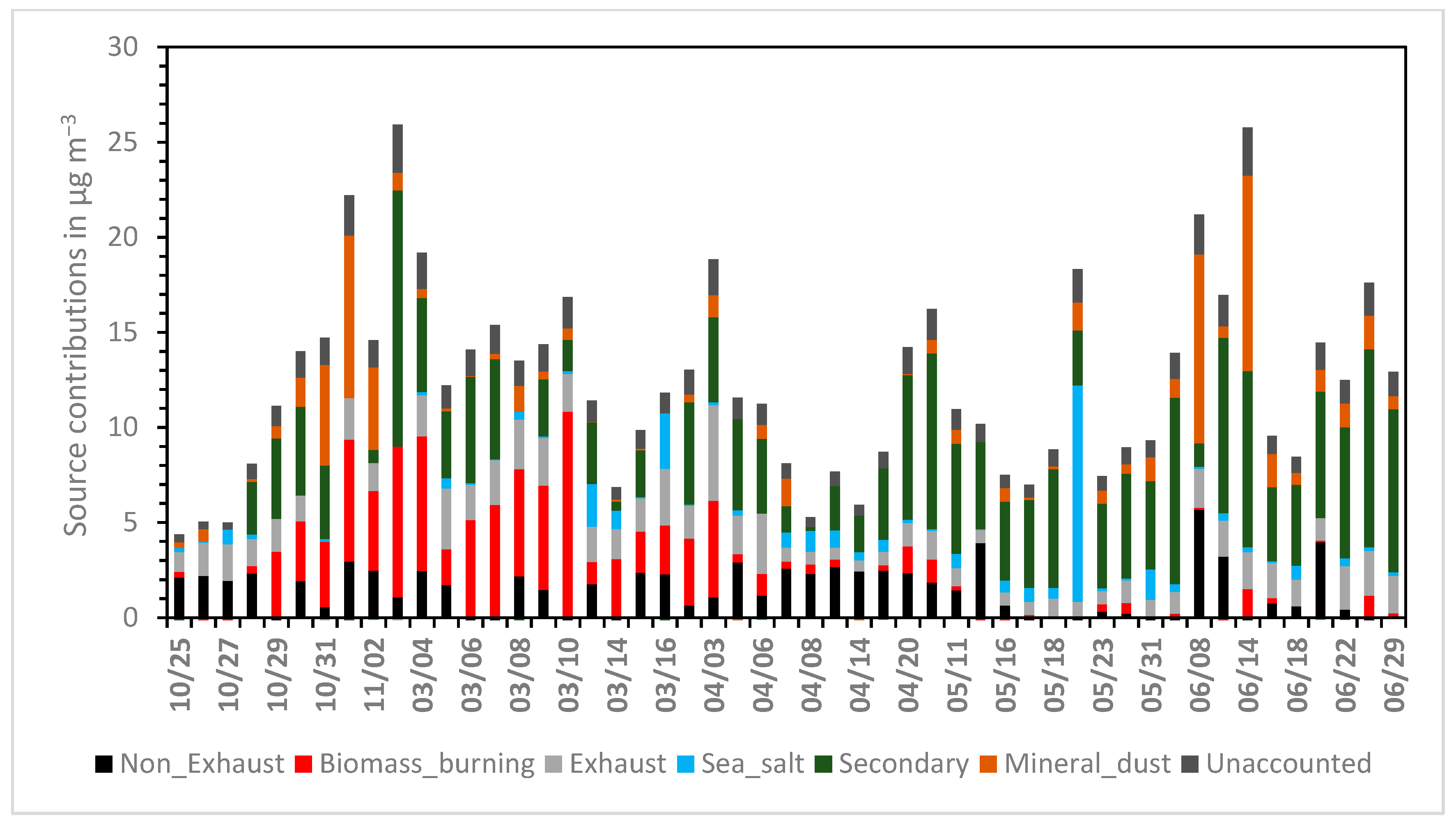
3.2. PM2.5 Source Apportionment

Six factors (Figure 1) were identified by the EPA PMF model using 55 samples and the 17 aerosol components shown in Table 1. No species were down-weighted. Because the number of samples used was close to the lower acceptable limit for PMF analysis, the solution was thoroughly evaluated to make sure that the overall and rotational ambiguity uncertainties were low. The low number of samples may have limited the number of identified sources and also increased the uncertainty of the analysis [36]. The number of factors was decided after the investigation of a range of possible solutions starting from four factors up to nine. Six factors were found to be the highest number of factors with a physical meaning, and resulted to the lower unaccounted mass estimation. The differences between Qtrue and Qrob and also between Qtrue and Qthe were less than 5%. One hundred simulations were performed and the differences in scaled residuals between the different simulations were very low. The results of the diagnostic tools offered by EPA PMF revealed that the solution was robust with low rotational ambiguity. Bootstrap results indicated that the factors were reproduced at a minimum level of 85% of the produced resamples, while displacement and bootstrap-displacement showed no factor swaps for the minimum dQ level. The PM mass reconstruction was satisfactory. The R2 between modeled and measured PM2.5 mass was 0.75 and the slope equal to 0.97. The composition of the six factors and the contribution of each factor to the concentration of each species are shown in Figure 1.
Factor 1 is characterized by the relatively high levels of Cu, Zn, Pb, Cr, Mn, Fe, and EC. All these elements are known to originate from the mechanical abrasion of different moving parts of the vehicles, such as tire and brake-wear, as well as the use of lubricant oils [37,38]. This factor was therefore assigned to non-exhaust transportation emissions. The average contribution of this source to PM2.5 was 12% (1.4 μg m−3).
Factor 2 is attributed to biomass burning because it is characterized by the relatively high levels of EC, OC, and K in the factor. The presence of tracers like Cr, Zn, and Pb in this factor may indicate some mixing with other sources. Since the contributions of these tracers in the factor profile are small, these mixing uncertainties should have only a minor effect on the estimated factor concentrations. The average contribution of the source to PM2.5 is 15% (1.9 μg m−3). Contribution of biomass burning was found to be higher than the contribution reported for the same site in 2011 (11%), which might be an effect of the economic crisis in Greece.
The contribution of this factor was quite high during the high PM2.5 periods of November 2018 and March 2019 (Figure 2). This was probably due to the burning of agricultural waste (mainly olive tree branches), but also to some domestic heating (fireplaces and woodstoves). PMF cannot separate agricultural burning from residential burning since their chemical profiles are very similar to each other. Some additional insights about the contributions of these two sources (agricultural burning versus residential heating) may be obtained from the analysis of the temporal profiles of the OA concentrations based on the AMS measurements. These will be discussed in a subsequent section.
Factor 3 is characterized by high levels of OC and EC and assigned to transportation exhaust emissions. Some elements originating from non-exhaust emissions, such as Cr, Mn, Cu, and Pb, are also present in the factor, but their contribution to the overall mass concentration is minor. The average contribution of this factor to PM2.5 is 13% (1.6 μg m−3) during the study period. The contribution is relatively stable, something expected given the lack of a seasonal pattern for these emissions.
Factor 4 is identified as sea salt and characterized by the presence of Na and Cl. Ni is also present in the factor, which might be an indication that this factor also includes some shipping emissions. Previous studies conducted in Patras have estimated that shipping emissions contributed approximately 4% to PM10 [8]. The concentration of vanadium, a good tracer of shipping emissions, was below the detection limit for a large number of samples, and could not be used reliably as a tracer in the PMF analysis. The average contribution of this marine source to PM2.5 was 5% (0.6 μg m−3). The high sea salt contribution observed on 19 May might be associated with high sea breezes or favorable meteorological conditions for sea salt generation and transport to the site.
The next factor (Factor 5) is characterized by the high contribution of sulfur and is identified as secondary sulfate. EC, Ni, and Na are also present in this factor, indicating that it may also include some contribution from shipping emissions. The combustion of residual oil used for shipping will produce particles containing V and Ni. Vanadium reacts with the oxygen from the combustion air surplus creating V2O5 that form layers on the heat exchanger and other boiler and stack surfaces. The V2O5 acts as a catalyst accelerating the SO3 formation, and therefore sulfate formation [39]. This factor has the highest contribution of 34% (4.2 μg m−3) to the average PM2.5 in the area. Its contribution can be compared with the concentration of 3.8 μg m−3 for sulfate, based on the measured sulfur.
Factor 6 is identified as mineral dust, and it is characterized by Al, Si, Ca, Ti, and Fe. All of these elements are related to mineral dust. The average contribution of the factor is 10%, and it contributes 1.3 μg m−3 to the average PM2.5. This is lower than the contribution of the sum of oxides above (19%), something reasonable given that some of the elements used for the calculation of the sum are attributed by PMF to sources other than mineral dust. This sum of oxides can be thus viewed only as an upper limit of the mineral dust contribution. The contribution of mineral dust was high on 11/01, 06/08, and 06/14. For those days the HYSPLIT backward trajectories indicated dust transport events from Africa. These Sahara dust events are common to Southern Europe in general and in Greece in particular [40].
The uncertainty of the solution was thoroughly evaluated using standard methods of the PMF analysis, since the number of samples used was relatively low. The results of the uncertainty analysis can be found in the Supplementary Material (Text S1 and Table S1). The unaccounted mass concentration was 1.4 μg m−3, which corresponds to 11% of the total PM2.5 mass. This is indicative of the order of magnitude of the uncertainty of our analysis.

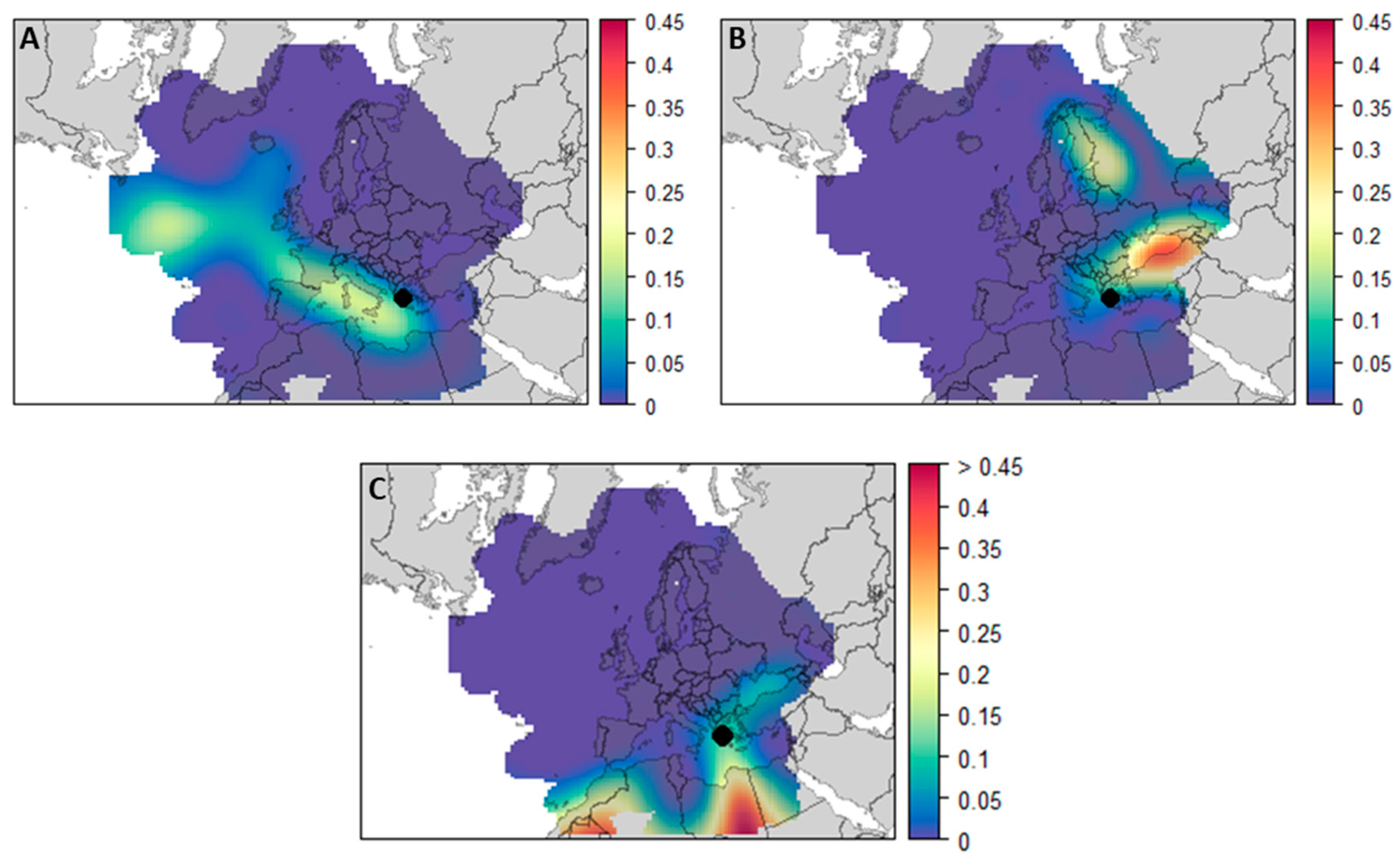
3.3. The Role of Long-Range Transport

To identify if the high-intensity events for the mineral dust, secondary sulfate, and sea salt factors were related to long-range transport, the PSCFs of their source contributions for the highest 15% concentrations were computed (Figure 3). The corresponding maps show the probability that a trajectory passing through the site was associated with one of the highest (top 15%) concentrations of the factor in the receptor. Sea salt during the high concentration period appears to have been transported to the sampling site from the Mediterranean Sea to the west. This is reasonable given that this factor should have a marine origin. The high concentrations of sulfates, on the other hand, were associated with transport from northwestern and northern Turkey, as well as the Black Sea region. There are a number of lignite-fired power plants with high emissions of SO2 in that area [41]. Emissions from the same areas were found to affect the concentrations of sulfates in different locations of Greece in the past [18].
Finally, the highest concentrations of mineral dust appear to have been related to transport from northern Africa. These Saharan dust events are known to affect Greece [15,40,42], as well as other areas in Southern Europe [43,44]. It should be noted that our PSCF results help identify source areas that contribute to the highest concentrations. Of course, there are also local contributions to the corresponding concentrations.

3.4. Nonrefractory PM1 Chemical Composition
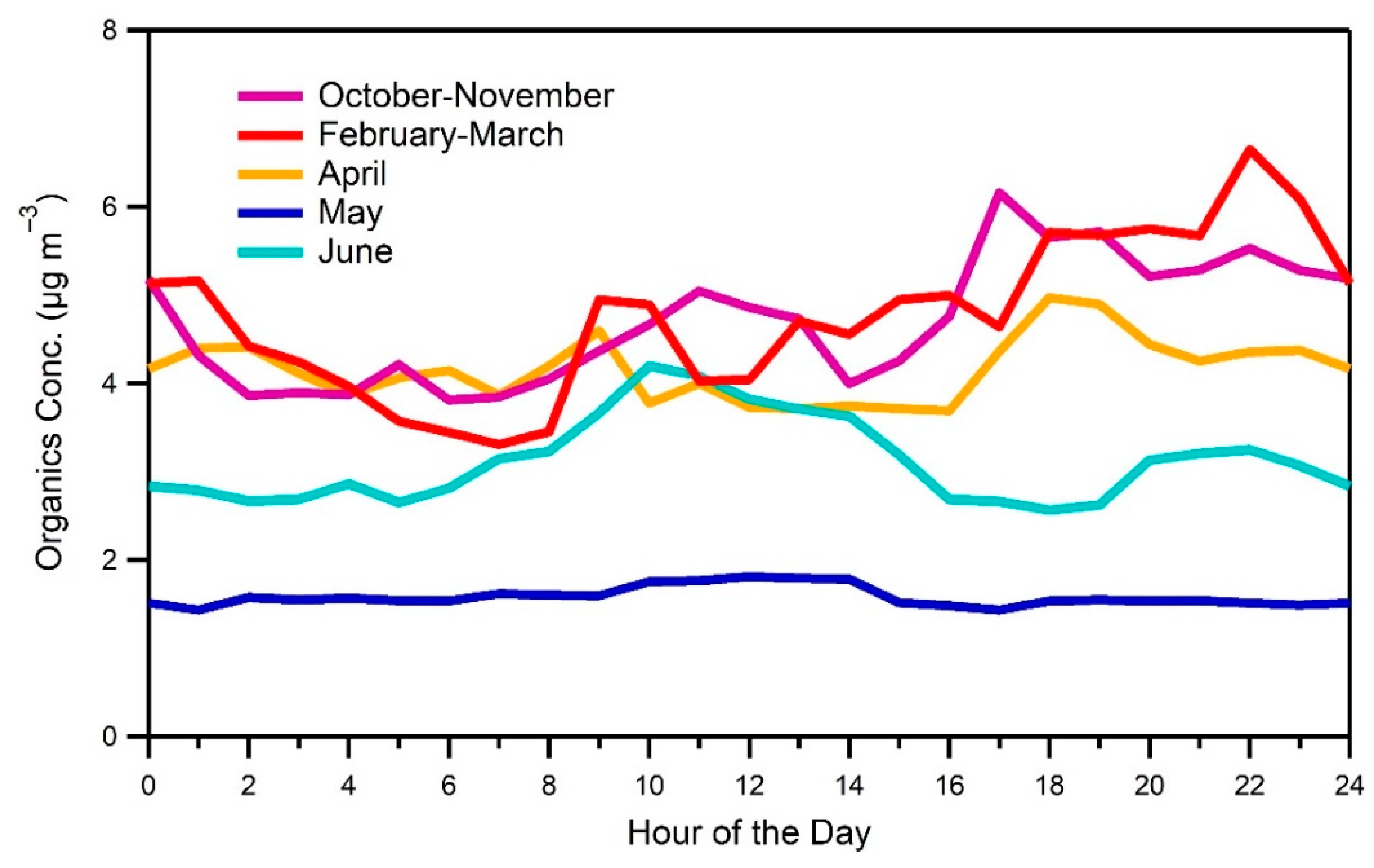
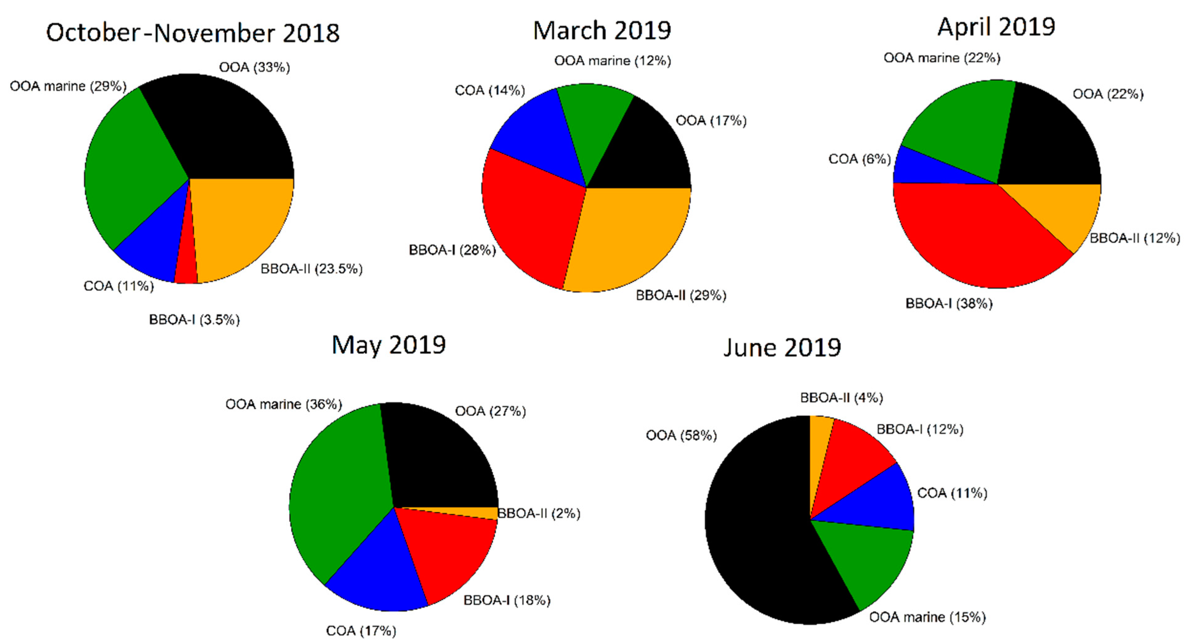
The average concentrations of the major nonrefractory PM1 (NR-PM1) components during the measurement periods are presented in Table 2. The average total NR-PM1 concentration during the sampling campaign was 7.7 μg m−3 ranging from 0.3 to 26 μg m−3 on an hourly average basis. The lowest NR-PM1 mass concentration values were recorded during May 2019 with an average concentration of 3.8 μg m−3. The highest concentrations were measured during the October–November 2018 period with an average NR-PM1 concentration of 9.9 μg m−3.
Organics (49%) and sulfate (35%) were the two major components of NR-PM1, followed by ammonium (13%) and nitrate (3%). These results are in general consistent with those from the analysis of the PM2.5 filters considering the differences in the size ranges (PM2.5 and PM1) and also the fact that the AMS does not measure the refractory PM components. OA was highest during November and March 2019, reaching hourly values as high as 20 μg m−3. Ammonium was present in sufficient concentrations to neutralize sulfate and had an average concentration of 0.96 μg m−3.
The nitrate concentration was relatively low with an average of 0.23 μg m−3 with the highest levels during the February–March period (0.45 μg m−3). Some of the differences between the PM2.5 and the NR-PM1 are due to the fact that elements like chloride often exist mainly in the 1–2.5 μm size range (in reality in the coarse mode) and are therefore part of the former and not the latter [45].
The average diurnal profiles of the OA during the sampling periods are shown in Figure 4. During May 2019, the OA concentrations are the lowest with a rather flat diurnal profile.
This suggests that they are mainly the result of long-range transport with small contributions of local sources or local production. The high concentrations of OA during October–November had a peak of around 6 μg m−3 at 17:00 and a minimum of around 4 μg m−3 in the early morning hours. During February–March, the high OA concentrations were during the night (from 18:00 to midnight), reaching a maximum of around 7 μg m−3 at 22:00 LT. The OA during June peaked at 10:00 in the morning while in April there was a morning peak at 9:00 and an afternoon peak at 18:00. These different patterns indicate the different sources and processes affecting the OA during different periods of the year and will be discussed further in the next section using the AMS spectra.
Additional insights about the contribution of biomass burning to the OA can be gained by examining the behavior of the m/z 60 (levoglucosan-related marker) in the AMS spectrum. The m/z 60 is a tracer of biomass burning OA and its diurnal average profile for the various periods of the study is shown in Figure 5. For May and June, the m/z 60 values are low and the diurnal profile is flat indicating that local biomass burning was not a major source of PM1. However, there is some regional biomass burning influence. In contrast, for the other periods (fall, winter, and spring) the m/z 60 has a notable diurnal cycle, with two peaks, one during the morning (9:00–11:00 LT) probably connected to local agricultural burning, and a second one during the evening.
The evening peak moves from the late afternoon (16:00–18:00 LT) during the spring and fall to the evening (23:00 LT) during the winter. This is consistent with agricultural burning being a significant source during the spring and fall, while residential heating increases in importance during the winter [22]. The diurnal AMS profiles add valuable information about the location of the biomass burning activities and some information about its sources that is not available from the analysis of the daily filters.
The O:C atomic ratio of the OA provides information both about its sources but also the processes influencing its concentration and chemical composition. The OA was in general quite oxidized (O:C equal to 0.82 on average) (Figure 6), a sign of important contributions of both long-range transport (aged OA) and secondary OA formation.
The lowest O:C values were observed for the February–March period with an average value of 0.73. The O:C peaked during the early morning (7:00 LT) at 0.79 and reached its minimum of 0.65 in the early evening (18:00). The highest average O:C of 0.91 was recorded during April. During this period, the O:C peaked during the afternoon (15:00 LT), a period associated with local photochemistry and at 4:00 LT. This second peak is more difficult to explain as it may be due to a reduction of local emissions of fresh, less oxygenated OA but also due to transport of more oxidized OA. The behavior of O:C during May and October–November was quite similar to that during April but with a little lower O:C value. Finally, the O:C during June also exhibited the two peaks (at 5:00 and 15:00 LT) but with even lower O:C values (the average was 0.77).
The density of OA was estimated using the Kuwata et al. equation [46] and the AMS O:C and H:C measurements, and was found to average 1.47 ± 0.09 g cm−3.

3.5. Sources of OA

PMF was applied to the high-resolution AMS organic mass spectra (m/z up to 200) for all the sampling periods. The determination of the PMF solution was based on the comparison of the spectra of the calculated factors to those of the literature, their physical meaning, their diurnal cycles, the correlation of the factor’s resulting time series with each other, and many other variables. The PMF resulted in a five-factor solution, including two oxygenated OA factors (an OOA, 30% and a marine-related OOA, 22%), a cooking OA (COA, 11%), and two biomass burning OA factors (BBOA-I, 19% and BBOA-II, 18%). The corresponding factor profiles are presented in Figure 7.
The two biomass burning OA factors contributed on average 37% to the total OA. Given that OA was approximately half of the NR-PM1, biomass burning was responsible for 19% of the NR-PM1 based on the analysis of the AMS data. This is quite consistent with the 17% contribution of the biomass burning to the PM2.5 estimated from the analysis of the filter samples. This contribution was quite variable, ranging from 57% during the February–March period to 16% during June (Figure 8). The different chemical composition of the two BBOA factors was probably due to a combination of different sources and different atmospheric processing (chemical aging). The BBOA-I factor was responsible for more than 75% of the BBOA during the spring and summer, approximately half of the BBOA during February–March, and just 13% during the fall.
The cooking OA factor contributed approximately 10% to the average OA from 6% to 17% of the OA depending on the sampling period. The maximum fractional contribution was recorded during May (17%) and minimum (6%) during April.
Most of the OA, according to the analysis of the AMS results, was oxygenated OA representing on average approximately half (52%) of the OA in the site. This oxygenated OA was either fresh secondary OA or aged primary and secondary OA transported to the site from other areas.
The OOA dominated the OA composition during the warmer months: 73% of the OA during June, 63% during May, and 62% during October–November. It represented 44% of the OA during April and 29% in February–March. This is consistent with its photochemical source. One of the two OOA factors resolved by PMF had contributions at m/z 64 and 80 (Figure 7), associated with marine OA and more specifically methanesulfonic acid (MSA) [47]. MSA is a product of the atmospheric oxidation of dimethyl sulfide (DMS) emitted by marine phytoplankton. This marine OOA was 40–60% of the total OOA during all periods with the exception of June, when it dropped to 20% of the OOA.
The average diurnal variations of all factors during the study are depicted in Figure 9. The OOA factor is the major contributor to PM1 with OA peaking at 12:00–14:00 LT. The second OOA factor peaks a little later at 16:00–17:00 LT. The behavior of both factors is consistent with the photochemical origin. Both BBOA-I and BBOA-II have a daytime peak (9:00–10:00 LT) and a second one at night (18:00–19:00 LT).
The COA factor has several small peaks throughout the day (10:00, 13:00, 17:00, and 22:00 LT). Some of them are related to Greek cooking hours, but some are not. The COA factor may also include the OA from local transportation, which was not identified by the PMF analysis of the AMS measurements. A hydrocarbon-like OA (HOA) factor was not identified even when we tried a six-factor solution. The COA factor AMS spectrum was quite similar to the others in the literature. As a consistency check, this factor reached high concentrations levels (around 8 μg m−3) during noon and the early afternoon of Fat Thursday, (28 February 2019) a day during which grilling meat is practiced throughout the city.

4. Conclusions

In the current study that took place in a suburban area of Patras, Greece, we quantified the sources of fine PM and its components based on both the elemental composition and EC/OC of the PM2.5, but also the sources of OA based on the high-resolution AMS spectra. The study covered periods during the whole year (from October 2018 to June 2019). The PM2.5 levels were modest with an average concentration of 12.4 μg m−3. The highest average PM2.5 was recorded during October–November (14.8 μg m−3) and the lowest during April (8.3 μg m−3).
Organics were the dominant PM component representing approximately 50% of both the PM2.5 and the nonrefractory PM1. Sulfates were the second most important component representing 35% of the NR-PM1 (based on the AMS) and approximately 25% of the PM2.5 (based on the XRF analysis of the filter samples). Ammonium was 12.6% of the NR-PM1 and nitrate levels were quite low, just 3% of the NR-PM1. The average EC was 0.38 μg m−3 contributing 3% to the PM2.5. The concentrations of 14 additional elements were quantified in the PM2.5 samples. Several of these components were expected to be mostly in the coarse PM mode and to contribute a lot more to PM2.5 (where the lower tail of the coarse mode is found) than to PM1.
The positive matrix factorization of the PM2.5 elemental composition together with the OC/EC data suggested six sources during the study period: secondary sulfate (34% of the PM2.5), biomass burning (15%), nonexhaust traffic emissions (12%), exhaust traffic emissions (13%), mineral dust (10%), and sea salt (5%). The PSCF analysis suggested that the high concentration periods of secondary sulfates were related to long-range transport of from northern and northwestern Turkey and the Black Sea region, of mineral dust transported from the Sahara, and of seasalt transported from the Mediterranean to the west of the site The relatively low number of filter samples increased the uncertainty of our PMF analysis. The unaccounted PM2.5 mass concentration was 1.4 μg m−3, which corresponds to 11% of the total.
The PMF analysis of the OA AMS mass spectra supported the importance of the biomass burning source. Two biomass burning OA factors were identified, contributing 37% on average to the PM1 OA. Given that OA was approximately half of the PM2.5, this estimate is consistent with that of the PMF, based on the elemental analysis. Both approaches suggested that the contribution of biomass burning was high during many of the high PM2.5 mass concentrations periods. Burning of agricultural waste and residential burning for heating contributed to the corresponding PM. Based on the diurnal profiles of the factors, agricultural waste burning was more prominent during the fall and spring, while residential burning increased in importance during the winter. The two factors identified may be due to different BBOA sources or a different degree of atmospheric processing (chemical aging). This should be investigated in future work.
The analysis of the AMS spectra suggested that approximately half of the OA was oxidized. Part of this OA was secondary and part was due to the oxidation of semivolatile primary OA emissions coming to the site from other areas. A part of the oxidized OA also included MSA, suggesting that it was also influenced by marine sources. This marine OOA should also be investigated in the future. Approximately 11% of the PM1 OA was due to cooking. The OOA and COA factors represented on average 62% of the OA, based on the AMS and they were not directly identified by the PMF of the elemental analysis, which included most of the OA in a factor traditionally attributed to nonexhaust transportation emissions. Interestingly, the analysis of the AMS data could not identify a fresh transportation OA factor (usually called hydrocarbon-like OA or HOA). The AMS analysis has difficulties in identifying sources that contribute less than 10% of the OA, so the HOA was probably low and was included in the COA but also in the BBOA or OOA factors. One possible explanation for the apparent difference in the predictions of the two methods is that a lot of the OOA was due to transportation sources, but not from the area of the study. If it was due to transport from other areas, there should have been enough time for the production of secondary OA from volatile and intermediate volatility organic compounds, but also for the oxidation of the semivolatile components of primary OA. A second explanation is that this factor characterized as nonexhaust transportation in many studies is not mainly due to transportation in this case, but rather is mostly secondary OA with some contributions from transportation. This is an important finding of this work that clearly deserves additional attention in future studies.
This study showcases the importance of using data for both the organic and inorganic components of PM to fully assess their sources. The next step should be the combination of that information into one single dataset, which might lead to the identification of more source-specific chemical profiles that assist in identifying and quantifying PM sources with higher accuracy. Inclusion of additional information such as PM size distribution could also be helpful.

Supplementary Materials

The following are available online at https://www.mdpi.com/2073-4433/11/4/330/s1, Text S1: Uncertainty Estimation of PM2.5 Source Apportionment, Table S1: Results of EPA PMF 5.0 uncertainty tools for source contributions to PM2.5 mass concentration (μg m−3).

Author Contributions

Conceptualization, S.N.P. and M.I.M.; methodology, M.I.M. and K.F.; validation, S.N.P., M.I.M., and K.F.; writing—original draft preparation, M.I.M. and K.F.; writing—review and editing, S.N.P.; supervision, S.N.P. All authors have read and agreed to the published version of the manuscript.

Funding

This research was financed by the European Union and Greek national funds through the program "Support for Researchers with Emphasis on Young Researchers" (call code: EDBM34), operational program "Development of Human Resources, Education and Lifelong Learning", NSRF 2014–2020, and under the research title: "Source apportionment of fine atmospheric aerosols and their organic component in urban and regional background areas in West Greece, for assisting air pollution and climate change long term management," MIS 5005098.

Conflicts of Interest

The authors declare no conflict of interest.

References

  1. Samoli, E.; Stafoggia, M.; Rodopoulou, S.; Ostro, B.; Declercq, C.; Alessandrini, E.; Díaz, J.; Karanasiou, A.; Kelessis, A.G.; Le Tertre, A.; et al. Associations between fine and coarse particles and mortality in Mediterranean cities: Results from the MED-PARTICLES Project. Environ. Health Perspect. 2013, 121, 932–938. [Google Scholar] [CrossRef]
  2. Samoli, E.; Stafoggia, M.; Rodopoulou, S.; Ostro, B.; Alessandrini, E.; Basagaña, X.; Díaz, J.; Faustini, A.; Gandini, M.; Karanasiou, A.; et al. Which specific causes of death are associated with short term exposure to fine and coarse particles in Southern Europe? Results from the MED-PARTICLES project. Environ. Int. 2014, 67, 54–61. [Google Scholar] [CrossRef]
  3. Katsouyanni, K.; Touloumi, G.; Samoli, E.; Gryparis, A.; Le Tertre, A.; Monopolis, Y.; Rossi, G.; Zmirou, D.; Ballester, F.; Boumghar, A.; et al. Confounding and effect modification in the short-term effects of ambient particles on total mortality: Results from 29 European cities within the APHEA2 Project. Epidemiology 2001, 12, 521–531. [Google Scholar] [CrossRef] [Green Version]
  4. Taghvaee, S.; Sowlat, M.H.; Diapouli, E.; Manousakas, M.I.; Vasilatou, V.; Eleftheriadis, K.; Sioutas, C. Source apportionment of the oxidative potential of fine ambient particulate matter (PM2.5) in Athens, Greece. Sci. Total Environ. 2019, 653, 1407–1416. [Google Scholar] [CrossRef] [PubMed]
  5. Cesari, D.; Donateo, A.; Conte, M.; Contini, D. Inter-comparison of source apportionment of PM10 using PMF and CMB in three sites nearby an industrial area in central Italy. Atmos. Res. 2016, 182, 282–293. [Google Scholar] [CrossRef]
  6. Belis, C.A.; Karagulian, F.; Larsen, B.R.; Hopke, P.K. Critical review and meta-analysis of ambient particulate matter source apportionment using receptor models in Europe. Atmos. Environ. 2013, 69, 94–108. [Google Scholar] [CrossRef]
  7. Amato, F.; Alastuey, A.; Karanasiou, A.; Lucarelli, F.; Nava, S.; Calzolai, G.; Severi, M.; Becagli, S.; Gianelle, V.L.; Colombi, C.; et al. AIRUSE-LIFE +: A harmonized PM speciation and source apportionment in five southern European cities. Atmos. Chem. Phys. 2016, 16, 3289–3309. [Google Scholar] [CrossRef] [Green Version]
  8. Manousakas, M.; Diapouli, E.; Papaefthymiou, H.; Kantarelou, V.; Zarkadas, C.; Kalogridis, A.-C.; Karydas, A.G.; Eleftheriadis, K. XRF characterization and source apportionment of PM10 samples collected in a coastal city. X-ray Spectrom. 2018, 47, 190–200. [Google Scholar] [CrossRef]
  9. Belis, C.A.; Pernigotti, D.; Pirovano, G.; Favez, O.; Jaffrezo, J.L.; Kuenen, J.; Denier van Der Gon, H.; Reizer, M.; Riffault, V.; Alleman, L.Y.; et al. Evaluation of receptor and chemical transport models for PM10 source apportionment. Atmos. Environ. X 2020, 5, 100053. [Google Scholar] [CrossRef]
  10. Gunchin, G.; Manousakas, M.; Osan, J.; Karydas, A.G.; Eleftheriadis, K.; Lodoysamba, S.; Shagjjamba, D.; Migliori, A.; Padilla-Alvarez, R.; Streli, C.; et al. Three-year long source apportionment study of airborne particles in Ulaanbaatar using X-ray fluorescence and Positive Matrix Factorization. Aerosol Air Qual. Res. 2019, 5, 1056–1067. [Google Scholar] [CrossRef] [Green Version]
  11. Favez, O.; El Haddad, I.; Piot, C.; Borave, A.; Abidi, E.; Marchand, N.; Jaffrezo, J.L.; Besombes, J.L.; Personnaz, M.B.; Sciare, J.; et al. Inter-comparison of source apportionment models for the estimation of wood burning aerosols during wintertime in an Alpine city (Grenoble, France). Atmos. Chem. Phys. 2010, 10, 5295–5314. [Google Scholar] [CrossRef] [Green Version]
  12. Paatero, P.; Tappert, U. Positive Matrix Factorization: A non-negative factor model with optimal utilization of error stimates of data values. Environmetrics 1994, 5, 111–126. [Google Scholar] [CrossRef]
  13. Crippa, M.; Canonaco, F.; Lanz, V.A.; Äijälä, M.; Allan, J.D.; Carbone, S.; Capes, G.; Ceburnis, D.; Dall’Osto, M.; Day, D.A.; et al. Organic aerosol components derived from 25 AMS data sets across Europe using a consistent ME-2 based source apportionment approach. Atmos. Chem. Phys. 2014, 14, 6159–6176. [Google Scholar] [CrossRef] [Green Version]
  14. Petit, J.E.; Favez, O.; Sciare, J.; Canonaco, F.; Croteau, P.; Močnik, G.; Jayne, J.; Worsnop, D.; Leoz-Garziandia, E. Submicron aerosol source apportionment of wintertime pollution in Paris, France by double positive matrix factorization (PMF2) using an aerosol chemical speciation monitor (ACSM) and a multi-wavelength Aethalometer. Atmos. Chem. Phys. 2014, 14, 13773–13787. [Google Scholar] [CrossRef] [Green Version]
  15. Manousakas, M.; Diapouli, E.; Papaefthymiou, H.; Migliori, A.; Karydas, A.G.; Padilla-Alvarez, R.; Bogovac, M.; Kaiser, R.B.; Jaksic, M.; Bogdanovic-Radovic, I.; et al. Source apportionment by PMF on elemental concentrations obtained by PIXE analysis of PM10 samples collected at the vicinity of lignite power plants and mines in Megalopolis, Greece. Nucl. Instrum. Methods Phys. Res. Sect. B Beam Interact. Mater. Atoms 2015, 349, 114–124. [Google Scholar] [CrossRef]
  16. Karanasiou, A.; Querol, X.; Alastuey, A.; Perez, N.; Pey, J.; Perrino, C.; Berti, G.; Gandini, M.; Poluzzi, V.; Ferrari, S.; et al. Particulate matter and gaseous pollutants in the Mediterranean Basin: Results from the MED-PARTICLES project. Sci. Total Environ. 2014, 488, 297–315. [Google Scholar] [CrossRef]
  17. Karanasiou, A.; Mihalopoulos, N. Air quality in urban Environments in the Eastern Mediterranean. In The Handbook of Environmental Chemistry 26; Viana, M., Ed.; Springer: Berlin/Heidelberg, Germany, 2013; pp. 219–238. [Google Scholar]
  18. Tsiflikiotou, M.A.; Kostenidou, E.; Papanastasiou, D.K.; Patoulias, D.; Zarmpas, P.; Paraskevopoulou, D.; Diapouli, E.; Kaltsonoudis, C.; Florou, K.; Bougiatioti, A.; et al. Summertime particulate matter and its composition in Greece. Atmos. Environ. 2019, 213, 597–607. [Google Scholar] [CrossRef]
  19. Kostenidou, E.; Florou, K.; Kaltsonoudis, C.; Tsiflikiotou, M.; Vratolis, S.; Eleftheriadis, K.; Pandis, S.N. Sources and chemical characterization of organic aerosol during the summer in the eastern Mediterranean. Atmos. Chem. Phys. 2015, 15, 11355–11371. [Google Scholar] [CrossRef] [Green Version]
  20. Kostenidou, E.; Kaltsonoudis, C.; Tsiflikiotou, M.; Louvaris, E.; Russell, L.M.; Pandis, S.N. Burning of olive tree branches: A major organic aerosol source in the Mediterranean. Atmos. Chem. Phys. Discuss. 2013, 13, 7223–7266. [Google Scholar] [CrossRef]
  21. Pikridas, M.; Tasoglou, A.; Florou, K.; Pandis, S.N. Characterization of the origin of fine particulate matter in a medium size urban area in the Mediterranean. Atmos. Environ. 2013, 80, 264–274. [Google Scholar] [CrossRef]
  22. Florou, K.; Papanastasiou, D.K.; Pikridas, M.; Kaltsonoudis, C.; Louvaris, E.; Gkatzelis, G.I.; Patoulias, D.; Mihalopoulos, N.; Pandis, S.N. The contribution of wood burning and other pollution sources to wintertime organic aerosol levels in two Greek cities. Atmos. Chem. Phys. 2017, 17, 3145–3163. [Google Scholar] [CrossRef] [Green Version]
  23. Saffari, A.; Daher, N.; Samara, C.; Voutsa, D.; Kouras, A.; Manoli, E.; Karagkiozidou, O.; Vlachokostas, C.; Moussiopoulos, N.; Shafer, M.M.; et al. Increased biomass burning due to the economic crisis in Greece and its adverse impact on wintertime air quality in Thessaloniki. Environ. Sci. Technol. 2013, 47, 13313–13320. [Google Scholar] [CrossRef] [PubMed]
  24. Canagaratna, M.R.; Jayne, J.T.; Jimenez, J.L.; Allan, J.D.; Alfarra, M.R.; Zhang, Q.; Onasch, T.B.; Drewnick, F.; Coe, H.; Middlebrook, A.; et al. Chemical and microphysical characterization of ambient aerosols with the aerodyne aerosol mass spectrometer. Mass Spectrom. Rev. 2007, 26, 185–222. [Google Scholar] [CrossRef]
  25. Canagaratna, M.R.; Jimenez, J.L.; Kroll, J.H.; Chen, Q.; Kessler, S.H.; Massoli, P.; Hildebrandt Ruiz, L.; Fortner, E.; Williams, L.R.; Wilson, K.R.; et al. Elemental ratio measurements of organic compounds using aerosol mass spectrometry: Characterization, improved calibration, and implications. Atmos. Chem. Phys. 2015, 15, 253–272. [Google Scholar] [CrossRef] [Green Version]
  26. Diapouli, E.; Manousakas, M.; Vratolis, S.; Vasilatou, V.; Maggos, T.; Saraga, D.; Grigoratos, T.; Argyropoulos, G.; Voutsa, D.; Samara, C.; et al. Evolution of air pollution source contributions over one decade, derived by PM 10 and PM 2.5 source apportionment in two metropolitan urban areas in Greece. Atmos. Environ. 2017, 164, 416–430. [Google Scholar] [CrossRef]
  27. Cavalli, F.; Viana, M.; Yttri, K.E.; Genberg, J.; Putaud, J.-P. Toward a standardised thermal-optical protocol for measuring atmospheric organic and elemental carbon: The EUSAAR protocol. Atmos. Meas. Tech. 2010, 3, 79–89. [Google Scholar] [CrossRef] [Green Version]
  28. Carslaw, D.C.; Ropkins, K. Openair—An R package for air quality data analysis. Environ. Model. Softw. 2012, 27, 52–61. [Google Scholar] [CrossRef]
  29. Stein, A.F.; Draxler, R.R.; Rolph, G.D.; Stunder, B.J.B.; Cohen, M.D.; Ngan, F. Noaa’s hysplit atmospheric transport and dispersion modeling system. Bull. Am. Meteorol. Soc. 2015, 96, 2059–2077. [Google Scholar] [CrossRef]
  30. Rolph, G.; Stein, A.; Stunder, B. Real-time environmental applications and display system: READY. Environ. Model. Softw. 2017, 95, 210–228. [Google Scholar] [CrossRef]
  31. Stohl, A. Trajectory statistics—A new method to establish source-receptor relationships of air pollutants and its application to the transport of particulate sulfate in Europe. Atmos. Environ. 1996, 30, 579–587. [Google Scholar] [CrossRef]
  32. Remoundaki, E.; Kassomenos, P.; Mantas, E.; Mihalopoulos, N.; Tsezos, M. Composition and mass closure of PM2.5 in urban environment (Athens, Greece). Aerosol Air Qual. Res. 2013, 13, 72–82. [Google Scholar] [CrossRef] [Green Version]
  33. Samara, C.; Voutsa, D.; Kouras, A.; Eleftheriadis, K.; Maggos, T.; Saraga, D.; Petrakakis, M. Organic and elemental carbon associated to PM10 and PM 2.5 at urban sites of northern Greece. Environ. Sci. Pollut. Res. Int. 2014, 21, 1769–1785. [Google Scholar] [CrossRef] [PubMed]
  34. Martins, V.; Faria, T.; Diapouli, E.; Manousakas, M.I.; Eleftheriadis, K.; Viana, M.; Almeida, S.M. Relationship between indoor and outdoor size-fractionated particulate matter in urban microenvironments: Levels, chemical composition and sources. Environ. Res. 2020, 183, 109203. [Google Scholar] [CrossRef] [PubMed]
  35. Viana, M.; Chi, X.; Maenhaut, W.; Querol, X.; Alastuey, A.; Mikuska, P.; Vecera, Z. Organic and elemental carbon concentrations in carbonaceous aerosols during summer and winter sampling campaigns in Barcelona, Spain. Atmos. Environ. 2006, 40, 2180–2193. [Google Scholar] [CrossRef]
  36. Belis, C.A.; Larsen, B.R.; Amato, F.; Haddad, I.E.; Favez, O.; Harrison, R.M.; Hopke, P.K.; Nava, S.; Paatero, P.; Prévôt, A.; et al. Air Pollution Source Apportionment with Receptor Models; Europena Union: Ispra, Italy, 2014. [Google Scholar]
  37. Manousakas, M.; Papaefthymiou, H.; Diapouli, E.; Migliori, A.; Karydas, A.G.; Bogdanovic-Radovic, I.; Eleftheriadis, K. Assessment of PM2.5 sources and their corresponding level of uncertainty in a coastal urban area using EPA PMF 5.0 enhanced diagnostics. Sci. Total Environ. 2017, 574, 155–164. [Google Scholar] [CrossRef] [PubMed] [Green Version]
  38. Pateraki, S.; Manousakas, M.; Bairachtari, K.; Kantarelou, V.; Eleftheriadis, K.; Vasilakos, C.; Assimakopoulos, V.D.; Maggos, T. The traffic signature on the vertical PM profile: Environmental and health risks within an urban roadside environment. Sci. Total Environ. 2019, 646, 448–459. [Google Scholar] [CrossRef]
  39. Kim, E.; Hopke, P.K. Source characterization of ambient fine particles at multiple sites in the Seattle area. Atmos. Environ. 2008, 42, 6047–6056. [Google Scholar] [CrossRef]
  40. Vasilatou, V.; Manousakas, M.; Gini, M.; Diapouli, E.; Scoullos, M.; Eleftheriadis, K. Long term flux of Saharan dust to the Aegean sea around the Attica region, Greece. Front. Mar. Sci. 2017, 4, 42. [Google Scholar] [CrossRef] [Green Version]
  41. Say, N.P. Lignite-fired thermal power plants and SO2 pollution in Turkey. Energy Policy 2006, 34, 2690–2701. [Google Scholar] [CrossRef]
  42. Mitsakou, C.; Kallos, G.; Papantoniou, N.; Spyrou, C.; Solomos, S.; Astitha, M.; Housiadas, C. Saharan dust levels in Greece and received inhalation doses. Atmos. Chem. Phys. Discuss. 2008, 8, 11967–11996. [Google Scholar] [CrossRef] [Green Version]
  43. Nava, S.; Becagli, S.; Calzolai, G.; Chiari, M.; Lucarelli, F.; Prati, P.; Traversi, R.; Udisti, R.; Valli, G.; Vecchi, R. Saharan dust impact in central Italy: An overview on three years elemental data records. Atmos. Environ. 2012, 60, 444–452. [Google Scholar] [CrossRef]
  44. Rodriguez, S.; Querol, X.; Alastuey, A.; Kallos, G.; Kakaliagou, O. Saharan dust contributions to PM10 and TSP levels in Southern and Eastern Spain. Atmos. Environ. 2001, 35, 2433–2447. [Google Scholar] [CrossRef]
  45. Eleftheriadis, K.; Ochsenkuhn, K.M.; Lymperopoulou, T.; Karanasiou, A.; Razos, P.; Ochsenkuhn-Petropoulou, M. Influence of local and regional sources on the observed spatial and temporal variability of size resolved atmospheric aerosol mass concentrations and water-soluble species in the Athens metropolitan area. Atmos. Environ. 2014, 97, 252–261. [Google Scholar] [CrossRef]
  46. Kuwata, M.; Zorn, S.R.; Martin, S.T. Using elemental ratios to predict the density of organic material composed of carbon, hydrogen, and oxygen. Environ. Sci. Technol. 2012, 46, 787–794. [Google Scholar] [CrossRef]
  47. Huang, S.; Wu, Z.; Poulain, L.; Van Pinxteren, M.; Merkel, M.; Assmann, D.; Herrmann, H.; Wiedensohler, A. Source apportionment of the organic aerosol over the Atlantic Ocean from 53° N to 53° S: Significant contributions from marine emissions and long-range transport. Atmos. Chem. Phys. 2018, 18, 18043–18062. [Google Scholar] [CrossRef] [Green Version]
Figure 1. Factor profiles obtained by Positive Matrix Factorization (PMF) using the EC, OC, and elemental concentrations. The bars represent the normalized concentration of the species in the profile and the circles show the contribution of the source to the average species concentration.
Atmosphere 11 00330 g001
Figure 2. Daily average source contributions to PM2.5 (μg m−3) determined by PMF of the elemental composition and OC/EC levels.
Atmosphere 11 00330 g002
Figure 3. Potential Source Contribution Functions (PSCFs) for the 85th percentile of (A) sea salt, (B) secondary sulfate, and (C) mineral dust factors.
Atmosphere 11 00330 g003
Figure 4. Average diurnal profiles of the OA during different periods of the study based on the Aerosol Mass Spectrometer (AMS) measurements.
Atmosphere 11 00330 g004
Figure 5. Diurnal variation of m/z 60 (related to levoglucosan), a tracer of biomass burning, in μg/m3.
Atmosphere 11 00330 g005
Figure 6. Diurnal variation of O:C of the organic aerosol based on the AMS measurements for the different periods of the study.
Atmosphere 11 00330 g006
Figure 7. Source profiles of OA factors determined by PMF of the AMS organic spectra.
Atmosphere 11 00330 g007
Figure 8. Average contributions of the various OA factors to total OA for the different sampling periods.
Atmosphere 11 00330 g008
Figure 9. Diurnal variation of OA factors determined by the AMS analysis for the whole study period.
Atmosphere 11 00330 g009
Table 1. Average PM2.5 mass concentration and composition during the study (all in μg m−3).
PM2.5ECOCNaMgAlSiSClKCa
Average12.400.382.850.35<0.100.290.710.920.120.170.10
Standard Deviation6.460.201.630.27-0.290.640.470.310.140.13
TiVCrMnFeNiCuZnBrSrPb
Average0.02<0.010.010.020.100.020.060.05<0.05<0.050.04
Standard Deviation0.02-0.000.000.110.010.030.05--0.01
Table 2. Average concentrations of nonrefractory PM1 (NR-PM1) components for the sampling periods.
Ammonium
(μg m−3)
Sulfate
(μg m−3)
Organics
(μg m−3)
Nitrate
(μg m−3)
Chloride
(μg m−3)
NR-PM1
(μg m−3)
October–November 20181.23.74.70.240.059.9
February–March 20180.952.54.70.450.098.7
April 20191.042.84.20.220.038.3
May 20190.61.61.60.090.023.8
June 20190.962.73.10.10.016.9
Average0.962.73.70.230.047.7

