Article

Modeling Land Suitability for Vitis vinifera in Michigan Using Advanced Geospatial Data and Methods

1
Department of Geography, Environment, and Spatial Sciences, Michigan State University, East Lansing, MI 48825, USA
2
Remote Sensing and GIS Research and Outreach Services, Michigan State University, East Lansing, MI 48823, USA
3
Department of Horticulture, Michigan State University, East Lansing, MI 48824, USA
*
Author to whom correspondence should be addressed.
Atmosphere 2020, 11(4), 339; https://doi.org/10.3390/atmos11040339
Submission received: 18 February 2020 / Revised: 24 March 2020 / Accepted: 27 March 2020 / Published: 30 March 2020
(This article belongs to the Special Issue Viticulture and Climate)

Abstract

:
Michigan (MI) has a long history of diverse agricultural production. One of the most rapidly expanding and profitable agricultural crops, wine grapes (Vitis vinifera L.), has only been in cultivation across MI since the 1970s. As of 2014 more than 2100 acres of Vitis vinifera were growing statewide. With such success there is a push to rapidly develop more vinifera vineyards across the state. The industry is striving to have 10,000 acres in cultivation by 2024. This study presents a data-driven approach for guiding decision making to make this goal attainable. The study models land suitability across the state using environmental, climate, topographic and land use data to understand the most to least ideal portions of the landscape for vinifera establishment. The models are tested in 17 MI counties. The study found that land suitability for viticulture has expanded and therefore, viticulture can be extended beyond the traditional growing areas. This study suggests that warming temperatures have influenced land suitability and demonstrates the application and utility of GIS-based land suitability modeling in viticulture development. Maps produced in this study provide knowledge of the climate and environmental trends, which is critical when choosing where and what cultivar to grow. With such resources, growers can be better prepared to invest and expand this pivotal agricultural sector.

1. Introduction

Viticulture is an important economic agricultural sector in many regions of the world [1]. It has been practiced for over 6000 years [2,3], largely in regions with specific climatic characteristics [2]. White et al. [4] reported that such regions have (a) adequate heat accumulation, (b) low risk of frost occurrence and (c) no extreme heat occurrences. The climates of these regions are integrally important in the concept of terroir—the notion that the quality and style of wine from a specific region is defined by complex interactions between the region’s physical and cultural factors [5]. While it is possible to grow grapes under more variable climates, the world’s best-quality wines require a certain balance amongst the three aforementioned climate conditions as these variables impact critical aspects of grape phenology [2]. Most of the suitable grape growing regions are found within 30–50° N and 30–40° S latitudes [5,6] although grapes have been grown elsewhere in the tropics as well [2].
Climate change and variability is projected to significantly impact agriculture, including viticulture [7]. Global grape production areas have experienced substantial climatic changes in recent years, with warming trends observed in most viticultural production regions [2]. Specifically, temperatures are projected to warm even more in most areas in the future, with increases of approximately 1.4 to 5.8 °C by the end of this century [8]. As global temperatures continue to rise, areas originally unsuitable because of insufficiently warm climates are gaining the ability to support grape production [9]. As a result, viticulture has expanded beyond regions traditionally bounded by the 10 °C and 20 °C isotherms [2]. Yet, the extent and levels of this changing land suitability is not well understood.
The International Organisation of Vine and Wine (OIV) Statistical Report on World Viticulture [10] reports that since 2014, the area under viticultural production in the United States has stagnated at approximately 440,000 hectares and 7 million tons (about 4.5 million tons of which are wine grape), respectively. Traditionally, California, Washington, Oregon and New York account for the majority, 94%, of U.S.-based grape production [9]. However, the wine industry is very dynamic. Over the last few decades, the number of vineyards has substantially increased, and new wine regions have emerged—especially areas known to experience harsh winter conditions, short growing seasons, high elevations and desert conditions [11]. Among these areas is the state of MI, in which vinifera wine grape production was unthought of back in the 1960s [12]. In this cool-climate region, a warming trend has been revealed by Schultze, Sabbatini and Andresen [13]. Here, growing degree day (GDD) accumulations have significantly increased from 1300–1500 in 1950s–60s to over 1600 in 1980–2011. This warming trend places MI in the “zone of transition” from being able to support primarily one species of grape (Vitis labrusca) to being suitable for production of a wide range of vinifera varieties [9]. As such, over the past few decades, MI has gone from unthinkable for wine grape production to one of the largest producers in the United States [12], ranking thirteenth in 2012 [13].
As Nesbitt, Dorling and Lovett [6] and Jones, Snead and Nelson [14] note, terroir in the longer-existing viticultural regions was defined through trial and error, experience, learning and adaptation over centuries. Therefore, expanding vinifera production to 10,000 cultivated acres in MI within a few years may be challenging, considering spatial variability in occurrence of specific environmental and climate conditions that vinifera need to do well. For instance, there is spatial variation in the warming trends and, therefore, growers are faced with the challenging task of identifying areas with suitable climate conditions (e.g., growing-season length, precipitation, temperature, occurrence of frost and snow events among others) for vinifera production. Besides this, growers also need to identify areas with specific topographic (e.g., slope, elevation and aspect) and soil characteristics that would enable production. On the other hand, geographic information systems (GIS) and remote sensing technologies have enabled multiple variables to be assessed and combined objectively in order to identify, rank and quantify suitability of land for certain uses. Since the cost of establishing a vineyard is high [15], poor decision-making can be financially devastating to the grower [16]. Therefore, it is critically important for growers to be able to assess land suitability for vinifera production, and the utility of GIS-based land suitability evaluation (LSE) is valuable in this endeavor.
LSE presents invaluable opportunities in agricultural land use planning. LSE models provide the much-needed information to growers and governments for better decision-making, especially as they struggle with pressures from increasing populations [17] and climate change and variability [18]. The models have been applied to assess land suitability for various crops including soybean production in Iran [19], rice in Pakistan [20] and Kenya [21], coffee in Central America [22] and Jamaica [23], maize in Kenya [24], shea in sub-Saharan Africa [25] among others. Within the viticulture sector, LSE has been used to assess suitability of land for vinifera production in England and Wales [6], North Carolina [15], the Umpqua Valley of Oregon [14], Jabal Al Arab in Syria [26] and Sarkoy in Turkey [27]. These studies generally integrate climate, soil and topographic variables in analyzing land suitability. Generally, variables are (i) reclassified based on their viticultural suitability; (ii) weighted based on their relative influence on viticulture and (iii) combined to generate final suitability maps. However, some differences exist. Some studies have used more objective methods for generating schemes for weighting variables. For example, analytical hierarchy process and pairwise comparison [26,27] have been used in this regard. Other studies [14,15] have opted to use expert knowledge specific to their study areas to generate weights for their model variables. In both cases, researchers have drawn valuable information from comprehensive literature reviews as well. Both methods are useful because, much as objective methods are recommended, terroir is delicately influenced by both the physical characteristics and cultural practices of a place, thereby making indigenous and expert knowledge necessary in understanding viticulture. Weighted sum has commonly been used to combine the weighted variables to generate final suitability maps (step iii above) [14,15,26,27]. The present study integrates expert knowledge specific to MI viticulture and climatology with information from Nowlin [15], Jones [28] and Jones, Snead and Nelson [14] among others to select, reclassify and weight variables used in the LSE models. Therefore, LSE models in this study are not new per se. However, no similar study has been conducted to assess land suitability for MI viticulture. Very high-resolution Light Detection and Ranging (LiDAR) topographic data used in this study has been made available only recently (since 2016), thus making it possible to model potential land suitability at very high (two-meter) resolution. As such, MI growers find this a systematic and novel approach in the attempt to improve viticulture and minimize economic losses related to climate change and variability.
This study introduces GIS-based LSE models for assessing potential land suitability for vinifera production in the state of MI. Primarily, the study tries to answer the question “What is the potential distribution of red and white vinifera varietals across the state given historical climate and land use and land cover (LULC) patterns?” To answer this question, the study utilizes advanced geospatial techniques and very high resolution remotely sensed data. In the study it is hypothesized that (i) red and white varietals exhibit different patterns of suitability and coverage across the state and (ii) the changing climate trends in MI have resulted in more suitable lands for vinifera cultivation over time. The models presented here are a holistic suitability assessment approach since climate, topography, soils and LULC are analyzed and integrated. The study tests the models on seventeen counties located along Lake Michigan and Lake Huron. It is key to mention that the four most important appellation areas of MI (Lake Michigan Shore, Fennville, Leelanau Peninsula and Old Mission Peninsula) are represented in this study. Final outputs from this study include a weighted matrix of ideal lands that can be used for cultivation of vinifera and will potentially serve as a decision-making guide for the viticulture industry in MI.

2. Data and Methods

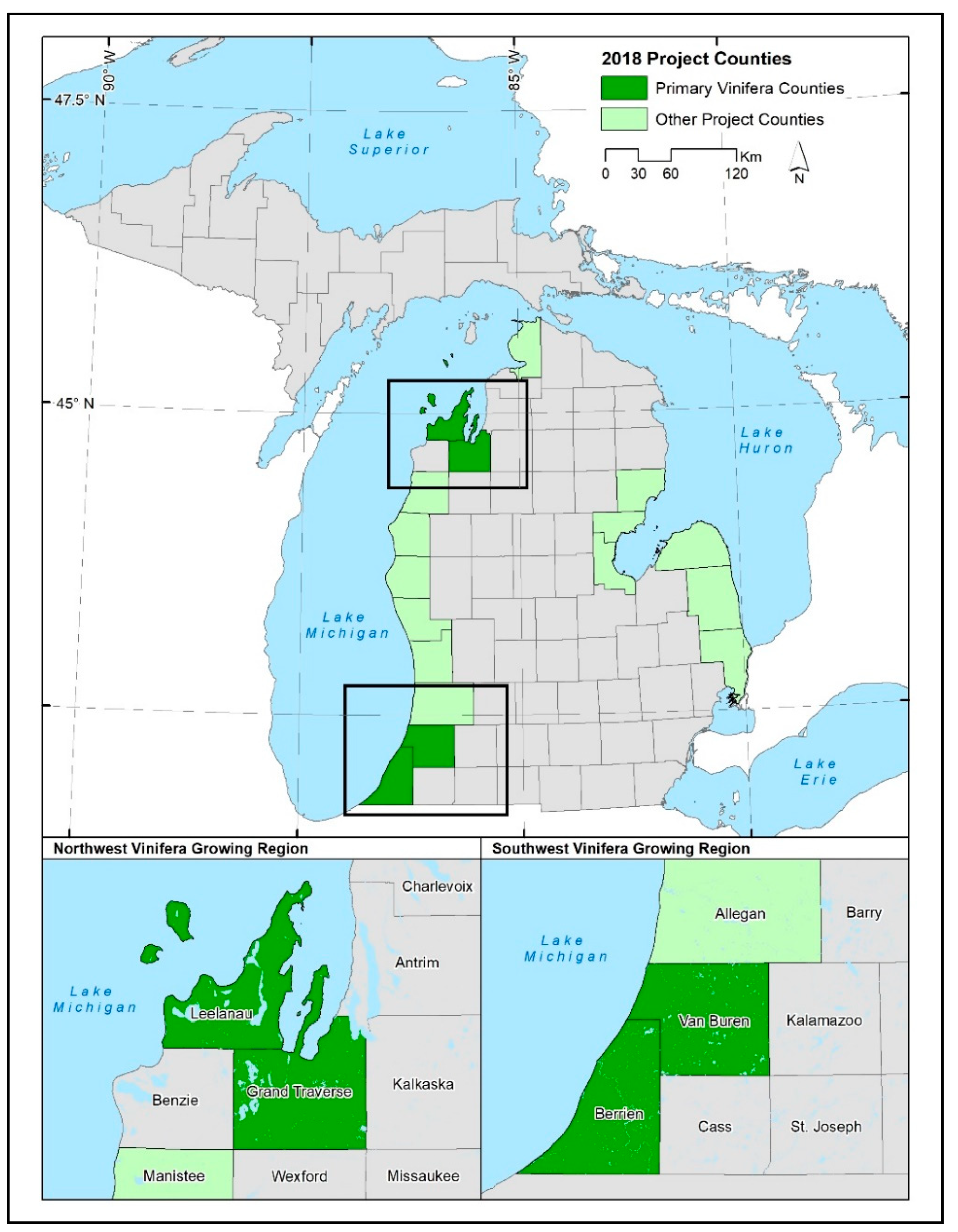
2.1. Study Area Characteristics

The present study was conducted in MI, United States. The region experiences a humid continental climate with warm summers, cold winters [9,13,16,29,30,31] and a mean growing season temperature range of 13 °C to 15 °C [9]. The region receives consistent precipitation year-round [29,31], estimated at 70–80 mm per month [32]. The presence of the Great Lakes substantially influences the state’s climate given changes in surface friction, heat and moisture content of upstream air flowing across large water surfaces—which in turn influences the amounts of cloud cover and solar insolation, air temperatures, precipitation and evapotranspiration downstream over the region [31,33]. Consequently, the “lake effect” significantly moderates MI’s climate throughout the year relative to locations farther from the lakes [9,31]. The region’s growing season is defined as the period between budburst and first fall frost [9]. The region also exhibits a variety of topographic characteristics, with hilltops and ridgetops at relatively higher elevations offering some protection against freezing temperatures due to cold air drainage. These topographic features, coupled with the Great Lakes modified climate, make it suitable for perennial fruit production including viticulture. Topographic aspect also plays an important role. For example, Schultze, Sabbatini and Andresen [13] report that cooler north- or east-facing slopes in northern MI may delay the timing of spring budburst and more sensitive phenological stages that follow, thus reducing the chances of damage associated with frosts. Additionally, the authors point out that southern-facing slopes in MI are warmer and promote earlier fruit ripening—which is important for a cool-climate growing region.
Historically, MI was unsuitable for vinifera grape production for four reasons. First, the region experienced low temperatures during growing seasons. Schultze, Sabbatini and Luo [29] report that in the 1950s and 1960s, the mean growing season temperature was 14.1 °C in the northwest corner of the Lower Peninsula and 16.5 °C in southwest MI. Low growing season temperature conditions can impact vine growth and reduce fruit technological maturity [9,16]. Secondly, the growing season was deemed too short with a general range of 140–160 days between budburst to first fall frost [13,29]. Thirdly, Schultze, Sabbatini and Luo [29] report that MI, especially the west coast, receives reliable rainfall all-year round. However, seasonal precipitation peaks coincide with veraison (beginning of fruit ripening) and harvesting periods leading to reduced yields due to increased fruit disease occurrence and failure of the vines to reach full fruit maturity [30]. Lastly, vinifera production is limited by occurrence of very cold winter temperatures [34]. These conditions have been common in MI [35] and have posed significant risks to viticulture, especially for the cold-tender cultivars of vinifera [34].
In general, the proximity of the Great Lakes results in more continental and variable (and viticulturally less suitable) climatic conditions across inland sections of the state’s Lower Peninsula [31]. Therefore, the LSE models presented in this study were tested on seventeen counties along Lake Michigan and Lake Huron shorelines and contain the vast majority of historical vinifera production areas in the state (Figure 1). The counties included Berrien, Van Buren and Allegan located in southwestern MI; Ottawa, Muskegon, Oceana and Mason (in western MI); Grand Traverse, Manistee and Leelanau (northwestern MI); Emmet (northern MI); Iosco and Arenac (northeastern MI); Bay (central MI) and; Huron, Sanilac and St. Clair (in eastern MI). The choice of these counties was influenced by availability of LiDAR-derived elevation data, collected through a collaboration between federal agencies and the state of MI, on which the study relies heavily. This data constraint limited the study area, but still allowed authors to assess a variety of different growing regions.

2.2. Data Sources

Fourteen variables were used in this study to determine environmental suitability. These were extracted from datasets obtained from Parameter-elevation Regressions on Independent Slopes Model (PRISM) [36] for the period 1982–2018, United States Department of Agriculture (USDA) Soil Survey Geographic database (SSURGO) [37] created in 2000, National Oceanic and Atmospheric Administration (NOAA) Coastal Change Analysis Program (C-CAP) [38] created in 2016, National Wetlands Inventory (NWI) [39] created in 2016 and United States Geological Survey (USGS) LiDAR [40] for the period 2016–2019. The variables and data are described in Table 1 below. The data was preprocessed before being integrated in the final LSE models. Please refer to Figure 5 and Appendix B for a description of the preprocessing procedures.

2.3. Model Development

2.3.1. Variable Selection and Reclassification

Climate is a major, and realistically the most important, factor in determining land suitability for the production of all agricultural crops [28]. In viticulture, it plays a critical role in regulating fruit ripening to achieve optimal characteristics for specific wine styles [28,41]. Therefore, climate is considered the most important aspect in terroir as it causes significant differences in wine styles [28]. As earlier stated, viticulture is practiced in regions with (a) adequate heat accumulation, (b) low risk of frost occurrence and (c) no extreme heat occurrences [4]. These conditions are discussed in detail by Jones [28] and key points are discussed below.
  • The rate and amount of solar insolation is critical in maintaining proper levels of photosynthesis—thus source of energy required for grape growth and maturation. Beginning at bloom, the amount of solar insolation is critical as it determines how tissue differentiation occurs and can cause coulure (failure of grapes to develop after flowering). During the ripening stage, insolation influences the amount of sugar (and in turn, potential alcohol content) formed in the grapes.
  • Length and temperatures of the growing season significantly influence grape ripening and quality of the fruits. To achieve optimum ripening, each grape cultivar should be grown in its specific ideal climate. The growing season length varies, but generally occurs within 170–190 days, with average temperatures greater than −1.1 °C for the coldest months and 18.9 °C for the warmest months. Generally, grapevines can withstand a minimum winter temperature ranging from −5 °C to −20 °C, with a high chance for damage for readings below −20 °C. While high temperatures (above 30 °C) boost the ripening potential of the berries, they may result in premature veraison due to heat stress. Even higher temperatures (above 35 °C) inhibit photosynthesis, thus negatively affecting plant growth, development and wine grape production. Effects of temperature dynamics on viticulture were also discussed by Belliveau, Smit and Bradshaw [42]. In another discussion of viticulture requirements, Nowlin [15] reports that temperature is the most important climate variable driving land suitability. It is mentioned that average annual minimum temperature, average annual maximum temperature, average annual temperature, growing degree days (GDD), frost-free period, last spring frost, first fall frost and spring frost index have been used in previous studies to assess temperature effect on viticulture. LSE models in the current study have incorporated GDD for both red and white vinifera varietals, frequency of cold days, frost-free days and mean spring temperatures.
  • Growing season precipitation is also important; rainfall occurrence during critical growth stages, while necessary, may also lead to devastating effects on wine grape production and quality. For example, ample rainfall is required for initial vegetative growth, but can slow down flowering during bloom. Rainfall can increase chances of fungal growth during berry growth and maturation stages. Moreover, rainfall can reduce sugar and flavor levels during maturation, thus resulting in lower quality [42]. LSE models presented here use two precipitation variables: (i) rainfall totals when rot is of critical concern and (ii) rainfall totals during key growth periods. Figure 2 shows the spatial patterns present in the six climate variables used in the LSE models.
Other studies have identified soil characteristics (including pH, drainage characteristics, nutrient and organic matter content, depth to bedrock and water holding capacity) as important factors in viticulture [6,14,43]. In their analysis, Jones, Snead and Nelson [14] considered drainage as most important relative to other soil variables. Importantly, models in the present study use all the above soil variables except water holding capacity and nutrient and organic matter content. Spatial patterns of the four variables are shown in Figure 3 below.
Land availability is an important consideration—mostly influenced by LULC and zoning characteristics, but also topographic characteristics. Accordingly, models in the current study exclude developed lands, water sources (rivers, streams, lakes, ponds and wetlands) and large topographic sinks. This exclusion is important as the study is more interested in potentially suitable land available for vinifera production. Slope and aspect have also been revealed as important variables in viticulture. Some studies have shown that these two variables influence solar and surface radiation balance especially during spring and fall [44]. Slope also influences cold air drainage and therefore controls the frequency and severity of frost events on a microscale [45]. For cool-climate growing areas like MI, south-facing slopes are important as they promote earlier fruit ripening [13]—since such slopes receive more solar radiation [12]. In their suitability analysis, Jones, Snead and Nelson [14] considered south-facing slopes ranging from five to 15 percent as most suitable for wine grape growth. The LSE models presented here incorporated slope, aspect and topographic sinks (depressions) in the analysis of land suitability for vinifera production. Figure 4 below shows the topographic variables for Grand Traverse County in northwestern MI. The figure also includes elevation from which the three topographic variables were generated.
After selecting and preprocessing, the model variables were reclassified into ten classes based on value ranges representing suitability conditions necessary for vinifera production. The outcome classes ranged from 0 (lowest suitability) to 10 (highest suitability). These classes were generated based on literature [14,15,28,41] and expert knowledge specific to MI. Excluded values were set to “NoData”. Table 2 below shows the classification schemes used to reclassify the variables. While class ranges were the same for both red and white varietals, note that different GDD ranges were used for the two varietals. The table (Table 2) compiles, for the reader, all the vinifera suitability requirements and reclassification schemes discussed above.

2.3.2. Variable Weighting

Based on literature reviewed above and expert knowledge specific to vinifera production in the state of MI, all variables but sinks were weighted, relative to each other. These weights indicate relative importance of each variable in vinifera production. Frequency of cold days was ranked highest with a weight of 10 followed by frost-free days and spring temperatures (both weighted 9). GDD, LULC and monthly precipitation during critical disease and rot periods were all given a weight of 8. Depth to bedrock was the lowest ranked variable (weight of 3). Final weights are presented in Table A1 in Appendix A. These weights were used to integrate the variables in the final LSE models.

2.3.3. GIS Model Development

The LSE models for vinifera production in MI were developed within a GIS environment. Data handling and analysis tools in ArcGIS software v10.6 [46] were used and the final models developed in ArcGIS ModelBuilder. The flowchart below (Figure 5) describes how each variable was preprocessed, analyzed, and integrated into the models to obtain final land suitability scores and maps.
To generate final vinifera suitability scores and maps for both white and red vinifera varietals, the study used weighted sum. For white vinifera, all variables except GDD for red vinifera were used. Here, each raster was multiplied by its weight (from Table A1 in Appendix A) and results summed. The same analysis was performed for red vinifera in which case GDD for white vinifera was replaced with GDD for red vinifera. The formula below generally shows how the final suitability scores were generated.
Final suitability score = ((a × aw) + (b × bw) + (c × cw) + (d × dw) + (e × ew) + …)
where a, b, c, d, e etc. are climate, topographic, land cover and soil variables discussed in Table 1. aw, bw, cw, dw, ew etc. are the corresponding variable weights (in Table A1 in Appendix A).
Theoretically, suitability scores could range from 0 to 880 due to the binning and weighting applied to the variables. Final suitability scores were reclassified into five suitability classes with equal ranges. These scores are shown in Table 3 below. Important to note is that both white and red vinifera varietal scores were reclassified using the same rubric.

3. Results

This study highlights, using LSE models, the potential land suitability for growing vinifera across the state of MI. Model results and maps quantitatively describe the spatial pattern of suitability and the differing drivers of such suitability. First discussed are descriptive statistics and maps of categorized variables used in the final LSE models. Land suitability statistics across counties are then summarized first by varietal and then by suitability class. Finally, some of the suitability maps generated from the LSE models are provided.

3.1. Model Variables Descriptive Statistics and Maps

Descriptive statistics of reclassified model variables are provided in Table 4 below. The study revealed very little variation across the study area in depth to bedrock and frequency of cold days. In terms of these two variables, the study area scored very highly for vinifera production (frequency of cold days had a class mean of 10 in all counties while depth to bedrock ranged between 9.97 and 10) indicating very high potential land suitability for vinifera production. Spatially, depth to bedrock had the least variation across counties (Figure 3). Depicting similar reclassification characteristics was depth of rooting zone with class means ranging from 8.89 (in Leelanau) to 9.98 (in Oceana). Appearing in the lowest classes (thus indicating lowest potential suitability) was aspect with values ranging from 0.61 for Leelanau and 3.21 for Muskegon. Soil drainage showed substantial variation in the classes, with values ranging from 0.75 in Bay to 7.73 in Emmett. The greatest variability across counties existed in GDD especially for red vinifera varietals. GDD for red vinifera had a minimum class mean of 1.12 (very low suitability) in Emmet County (northernmost county in the study) compared to a class mean of 10 (highest suitability) in Allegan, Berrien and Van Buren counties in southwestern MI. Similar patterns exist for white varietals for which GDD has a minimum class value of 1.4 in Emmet and at least 8 elsewhere.
Weighted sums for soil, topographic/land cover, and climate (for both red and white vinifera varietals) are presented in Figure 6 below. Clearly, there is a general north–south trend in potential climate suitability for vinifera production. Only subtle differences exist for climate suitability for red and white varietals. However, these differences drive very significant variations in land suitability for the two varietals. Distance from lakes also matters, and climate suitability reduces significantly as one moves inland—mainly evident in the northernmost portions of the Lower Peninsula. For topography and land cover, low values exist mostly in northern counties. In terms of the soils, southwestern, western and some northern counties score highly, although very low values exist in those northern counties as well.

3.2. Potenital Land Suitability by Varietal

The LSE models revealed that potential suitability for vinifera production in the study area ranges from 234 to 803 (for red varietals) and 234 to 789 (for white varietals). These scores depicted a general normal or near-normal distribution. It was also found that southwestern counties had higher scores compared to the rest. Higher potential suitability was found for red vinifera compared to white vinifera in Berrien, Allegan, Van Buren and Ottawa (Figure 7). These counties also had the highest mean suitability scores for the red varietal; mean scores of 636, 630, 630 and 598, respectively. This indicates a general medium-high suitability for red vinifera production in these counties. Suitability for the two varietals was generally similar in Bay, Emmet, Muskegon and St. Clair. Land suitability for white varietals was higher than that of red varietals in the remaining counties. Highest average suitability scores for white vinifera were obtained in Berrien (620), Van Buren (614), Allegan (614) and Mason (607). Lowest suitability scores were obtained in northern counties with Emmet County scoring the least (mean score of 498 and 500 for red and white varietals, respectively).

3.3. Potential Land Suitability by Class

The study found potentially suitable land for vinifera production totaling to 1.74 million hectares (all suitability classes). However, suitability is varied across the region and more than 75 percent of the land falls in the fourth suitability class (suitability score range = 529, 704), indicating medium-high suitability. There is less than one percent of the land in the medium-low suitability class for red varietals and is found in all counties except Allegan, Bay, Berrien, Mason and Van Buren. For white varietals, land in this class is spread across all counties except Allegan, Bay, Manistee, Mason, Oceana, St. Claire and Van Buren. Some land occurs in the high suitability class (values greater than 704), most of which is found in Allegan, Berrien, Van Buren and Ottawa (for red varietals) and Berrien, Leelanau, Mason and Allegan (for white varietals). No land was found in the low suitability category. Highest proportions of potentially suitable land were found in Sanilac (78 percent), Emmet and Allegan (both with 72 percent) (Figure 8 and Figure 9). However, most (about 70 percent) of the suitable land in Emmett was found in the medium suitability class. Least proportions were found in Iosco and Mason (both with 57 percent).
Different patterns exist when total area of potentially suitable land in each county is considered. For both varietals, the study found that Sanilac, Allegan and St. Clair had the highest total area. These counties had over 190,000, 150,000 and 130,000 hectares of potentially suitable land, respectively. Additionally, the study found that, for both varietals, Leelanau and Arenac had the lowest total area of suitable land (approximately 67,000 and 59,000 hectares, respectively). For red varietals, suitable land in Iosco is approximately equally distributed between medium and medium-high suitability classes. However, different patterns are visible for white varietals—there is significantly more land in the medium-high than the medium class in the county. Class-by-class comparisons across red and white varietals reveal that there is more than 10,000 hectares of land with high suitability for red than white varietals, most of which is in Allegan, Berrien and Van Buren. Besides, there is more than 70,000 hectares of land in the medium-suitability class for red compared to white varietals. These differences are compensated for in the medium-high suitability class in which there is more than 80,000 hectares for white compared to red varietals—mostly found in Sanilac, Allegan, St. Clair and Huron. The total amount of potentially suitable land for each county is the same for both varietals.

3.4. Potential Land Suitability Maps

An important deliverable for this study is the production of land suitability maps for vinifera production in the MI counties—with suitability calculated based on a multicriteria analysis of climate, topographic, soil and LULC variables. The study produced maps indicating weighted suitability scores for red and white vinifera varietals. Sample suitability maps are provided in Figure 10 (red varietals) and Figure 11 (white varietals). These maps represent potential suitability for vinifera production in Grand Traverse County (northern MI) and Berrien County (southwestern MI). Suitability maps for each of the seventeen studied counties are available online [47].

4. Discussion

4.1. LSE and Its Utility for the Viticulture Community

A warming trend in climate has been reported in viticultural regions across the world [1,4,5,6,9]. Since wine grapes are very sensitive to climate [48], this warming trend poses great challenges and opportunities for viticulture—including a geographical redistribution of viticultural regions [6,49], thus the rise of ‘new world’ viticultural regions in places initially thought to be unsuitable for wine grape production. Some of the new viticultural regions are the cool-climate regions where very few studies of climate change impacts on viticulture have been conducted [6].
Across the US, fruit crops are suffering and becoming uneconomically viable due to invasive pests destroying harvest, high production costs [50,51] and/or low prices [51]. Converse to this is vinifera cultivation, which has seen, in recent years, large increases in land under cultivation, established vineyards and wineries, and an overall greater acceptance/interest [52]. In 2011, vineyards in MI contributed $11.6 million to the state’s economy including adding more than 880 jobs [53]. Such economic impact has risen over the years as viniculture expands across the state. In their 2017, Economic Impact Study of the Michigan Wine Industry, John Dunham and Associates [54] found that the industry directly generated $2.1 billion in the state economic activity while employing about 28,000 people. With the industry’s interest in growing vinifera and new vineyard establishment, it is the ideal time to develop LSE modeling approaches.
Future growth of viticulture across the state of MI is dependent on the factors included in the current LSE models (climate, soil, and topography) as well as economics. There are thousands of varietals of Vitis vinifera [12]. With each varietal there are differences in their climate optimum as some may be better suited for wetter conditions and others for drier environments. With the generally warming climate, thus spatially varying occurrence of land suitability for viticulture, multi-criteria analyses like the LSE models presented here are necessary. Such models would assess, combine and evaluate a land parcel’s biophysical, topographic and soil characteristics necessary for viticulture. In order to make the LSE modeling operational across the state, and result in success for growers, a grower must first consider the variety they plan to grow in conjunction with the LSE modeling and associated variable weights [14,55,56,57,58]. While modeling efforts are now underway to study varietal-specific suitability across the state, there remains great utility in this version of the LSE. The most common varietals will have LSE models parameterized according to their climate and environmental optimums.
Overall, land suitability evaluations gauge suitability by scoring and weighting critical variables based on the literature and current landscape trends. Here there are different LSE models based on red and white varietals, as these two major varietals have differing optimal climate conditions–specifically growing degree day accumulations. In this study, regions of high suitability correspond to LSE values from 705 to 880. On the ground, these regions would not only have ideal climate regimes but also soils, hydrology, and/or topography. More specifically, across these regions, multiple variables of critical importance to the LSE are ideal for viticulture. For instance, these regions could have ideal climate and land use. Regions of low suitability correspond to values from 0 to 176 in the LSE models. It is not to say that vinifera cannot grow here, it is just a less optimal location based on the LSE model inputs. Likely, more climate-hardy varietals would have a better chance of survival in such a region. Across MI there are regions growing vinifera not included in the suitability surface. This lack of inclusion can occur for several reasons including, most notably, lack of topographic data. It is also noted that the LSE models developed in this study are not a definitive definition for where vinifera can be cultivated across the state. Instead the models are meant to guide growers and stakeholders on drivers of land suitability and spatial occurrence of potentially suitable regions.
Many studies exist in the literature that have assessed land suitability for viticulture. Some have found significant agreement between LSE results and existing vineyards [15,59], thus validating LSE methodologies used. Most of these studies found greater extents of suitable land for vinifera production [6,14,59]. As such, less land was used for vinifera production than was suitable based on climate, topography and soil characteristics. Results from the present study point to the same trend, as suitable land significantly extends beyond the traditional viticulture regions. Some studies have found that existing viticulture isn’t being practiced in the most suitable portions of land [6,27]. This may be because of a lack of prior LSE analyses in some cases [6], which would underscore the importance of LSE modeling in viticulture development. In other cases, the choice of a vineyard location is influenced by proximity to markets and availability of transport networks, which seem to override land suitability [27]. It is recognized that such factors are important in viticulture, but the present study did not include them in the LSE models, as well as evaluation of viticultural practices able to contrast or mitigate adverse climatic and soil characteristics. This is because the objective of this study was to model potential land suitability for vinifera production in MI, based solely on a combination of climate, topography, soils and land uses.

4.2. The Economic Investment for Vinfera

Viticulture has substantially grown into a global multimillion-dollar venture over the past three decades [3]. China, Italy, United States, Spain and France are the leading producers of grapes, accounting for 15%, 11%, 8.9%, 8.9% and 8% of global production, respectively [10]. Vitis vinifera is the most common cultivated grape species, making up approximately 90% of world grape production [3]. Given the economic importance of vinifera development, especially across multiple states in the US, it is important to understand the environmental settings ideal for its production.
The installation of a vineyard is expensive and time consuming. Vinifera is a perennial crop and to produce such a crop, there is a large establishment cost and even with establishment there are uncertainties about future production [15]. For instance, it takes two to three years for vines to produce fruit after establishment [60]. An additional one to two years thereafter are needed to reach their highest production potential [42,60]. Thus, establishment costs for a vineyard are high and such costs are not offset by quick revenue gains [57]. With the LSE, the study aims to assist growers in expanding their knowledge of the landscape to aid in viticulture development. The maps produced by the LSE models will not offset the high expense for vineyard development, but knowledge of the climate and environmental trends is critical when choosing where and what varietals to grow.
Conversely, while viniculture is a large investment for the grower, it also stimulates, when successful, the economy around the vineyard [53]. For example, Tuck and Gartner [53] mention that viticulture directly benefits the economy through purchasing of supplies and labor needed in the vineyards and wineries. Additionally, with successful viticulture development comes economic stimulus across multiple other sectors, most notably tourism. Meaning, though the LSE is intended to highlight suitable lands for viticulture, there is a potential secondary use. With the ripple effects that successful vineyard development has across a region’s economy, such LSE maps speak to potential opportunity for investment from other, associated, economic sectors.

4.3. LSE Model Limitations

The most important limitation in this study was the limited availability of precise topographic data. With time, this data is becoming more comprehensive, but during the study only a small number of county LiDAR datasets were available, thus greatly limiting the area of study. Besides, datasets used during this project varied in resolution/precision. For instance, PRISM data pixel resolution is 4 km, whereas LiDAR-derived digital elevation model (DEM) data is available at one meter from the USGS. To capture local-scale topographic information, it was necessary to resample climate score data to a higher resolution. Like every other location where vinifera LSE research has been conducted, MI is unique in terms of climate, soil, topography and LULC. For this reason, it was sometimes necessary to utilize expert knowledge rather than quantitative information when deciding upon the correct value ranges, weights and, finally, scores. Modeling occurred in both R and ArcGIS ModelBuilder. ModelBuilder, while simpler to use when creating logical expressions, is somewhat inefficient, particularly with large datasets. Future efforts would benefit from streamlining the process in Python [61], R or a similar programming language [62].
The soil data used in the present model is dated and this has limitations. County boundaries are clearly manifested in the results, thus indicating differences in sampling and/or data creation. Besides, while long term mean is ideal for some climate variables, extreme variations in weather may be overlooked and this may have catastrophic consequences on vine health—especially since vinifera is highly sensitive to very cold winter temperatures and excess rainfall.

5. Conclusions

It was long thought that MI was too cold, too wet at the wrong times of year, and had too short a growing season for viticulture to be sustained [29]. However, the MI wine industry has not only sustained itself in the past few decades but has grown drastically, with even more growth planned. Therefore, this study developed LSE models to highlight portions of the landscape potentially ideal for vinifera expansion, considering red and white varietals separately.
The models revealed that land suitability for viticulture has expanded and therefore, viticulture can be extended beyond the traditional growing areas. The study found that southwestern MI counties have the highest suitability while northern and northeastern counties indicate relatively lower suitability. Generally, potential suitability is lower for red compared to the white vinifera varietals. Land suitability for red varietals appears higher in southwestern counties as most of the land is in the medium-high or high suitability classes. It is noted that no clear spatial patterns exist for distribution of land in the high suitability category for white vinifera, although land in this class may appear weakly concentrated in western compared to eastern counties.
Overall, in the models in this study, the climate variables were most strongly weighted as vinifera production is greatly driven by temperature and precipitation regimes. Temperature factors, in this case frequency of cold days, spring temperatures, number of frost-free days, and growing degree days, are the most critical in determining a region’s suitability for viticulture. The importance of such variables in vinifera LSE models is not just seen within the state of MI. Studies (e.g., [14,63,64]) have long noted that climate, particularly temperature, is absolutely critical to understanding viticulture. This study therefore suggests that warming temperatures have greatly influenced land suitability for vinifera production in MI. Following temperature variables was precipitation. Precipitation is critical as its timing is essential for viticulture. Precipitation around the time of harvest can lead to fruit rot, whereas precipitation during the spring is ideal for vine growth and development. The other variables, soil and topography, are important to vinifera growth just to a lesser degree than climate.
This paper looks to assist the wine growers of MI in their goal to increase vinifera production to 10,000 cultivated acres by 2024 [65]. Achieving this goal is challenging, especially because of the changing climate patterns coupled with the specific biophysical conditions that vinifera require to thrive. However, authors believe that with more knowledge, such as that provided from the LSE models, the grower community can be better prepared to make sure an investment across the state of MI. Future work will perform similar LSE modeling by vinifera varietals, both red and white for the entire state of MI. Additionally, future work will utilize climate change projections data to model LSE for vinifera production into the future.

Author Contributions

Conceptualization, E.L.B., R.G. and N.W.; methodology, E.L.B., R.G., N.W., P.S. and J.A.A.; software, E.L.B., R.G., N.W. and D.W.; validation, E.L.B., R.G. and N.W.; formal analysis, E.L.B., R.G., N.W. and D.W.; resources, E.L.W.; data curation, E.L.B., R.G. and N.W.; writing—original draft preparation, D.W. and E.L.B.; writing—review and editing, D.W., E.L.B., R.G. and N.W.; visualization, R.G., N.W. and D.W.; supervision, E.L.W.; project administration, E.L.B.; funding acquisition, E.L.B., P.S., and J.A.A. All authors have read and agreed to the published version of the manuscript.

Funding

This research was funded by Michigan State Horticultural Society under Michigan State University (PD29534).

Acknowledgments

This research was funded thanks to a grant from the Michigan State Horticultural Society (MSHS) called “Modeling Michigan Suitability of Vitis Vinifera Using Advanced Geospatial Data and Methods.” There are multiple people and organizations that made this publication possible and the authors wish to express their gratitude, especially to Ben Smith from MSHS for your support and keen interest in the project. Additionally, the authors thank the reviewers for their time and effort put into the manuscript.

Conflicts of Interest

The authors declare no conflict of interest.

Appendix A

Final weights are presented in Table A1 below. These weights were used to integrate the variables in the final LSE models.
Table A1. Final variable weights used in the LSE models for vinifera production in Michigan.
Variable Weight
Frequency of Cold Days 10
Spring Temperatures 9
Frost-Free Days 9
Growing Degree-Days 8
Monthly Precipitation (Disease/Rot) 8
Land Cover and Land Use 8
Slope 7
Soil Drainage 6
Slope Aspect 6
Monthly Precipitation (Growth) 5
Soil pH 5
Depth of Rooting Zone 4
Depth to Bedrock 3

Appendix B

Data Preprocessing

All datasets were preprocessed in ArcGIS software v10.6 except PRISM. The latter was preprocessed in cran R. Preprocessing involved the following steps. It should be noted that all preprocessed and/or generated datasets were eventually resampled to 2-m spatial resolution.
  • Joining soil data attributes to soil polygons. Soil drainage, pH, depth of rooting zone and depth to bedrock information contained within soil description tables were joined to soil polygons using the muid field. The resulting joins were based on many-to-one relationships, meaning that many polygons could share the same attribute. Individual raster datasets were then generated for each soil variable.
  • Generating slope, aspect and sink data from LiDAR digital elevation model (DEM). Using surface tools within ArcGIS, percent slope and aspect data were generated. Hydrology tools in ArcGIS were used to generate a filled DEM. Raster math was then used to subtract the native DEM from the filled DEM to generate topographic depressions, otherwise known as sinks. Sinks are locations that accumulate both cold air and water.
  • Calculation of long-term means of PRISM temperature. PRISM data used covered the period from 1983 until 2018. Variables extracted include:
    • Frost-free days: This variable was calculated by generating the long-term mean of days from 1 April to 31 October where temperatures did not reach freezing (0 °C or less).
    • Frequency of cold days: Generated by calculating long-term mean of days when minimum temperature fell to −20 °C or below for the period from December 1 to February 28.
    • Spring temperatures: The variable was calculated by generating the long-term mean of average temperatures in °C for the period from 1 March to 30 June.
    • GDD: Calculated from long-term means of accumulated daily GDD values for the period between 1 April and 31 October. Original GDD values were calculated using the formula below.
      GDD = (Tmax + Tmin)/2 − Basetemp
      where Tmax, Tmin and Basetemp are maximum, minimum and base temperatures, respectively and all negative daily GDD values are set to 0. The base temperature used in this calculation is 10 °C (50 °F). Source: [66,67].
  • Calculation of long-term means and standard deviations of PRISM precipitation. From these statistics, the following variables were generated.
    • Precipitation—growth: This variable was calculated first as the long-term mean and then the long-term standard deviation of precipitation amount (in millimeters) in the month of June only.
    • Precipitation—rot: Calculated first as the long-term mean and then the long-term standard deviation of the amount of precipitation (in millimeters) from 1 August through 31 October.

References

  1. Fraga, H.; Malheiro, A.C.; Moutinho-Pereira, J.; Santos, J.A. An overview of climate change impacts on European viticulture. Food Energy Secur. 2012, 1, 94–110. [Google Scholar] [CrossRef]
  2. Schultz, H.R.; Jones, G.V. Climate induced historic and future changes in viticulture. J. Wine Res. 2010, 21, 137–145. [Google Scholar] [CrossRef]
  3. Venkitasamy, C.; Zhao, L.; Zhang, R.; Pan, Z. Chapter 6—Grapes. In Integrated Processing Technologies for Food and Agricultural By—Products; Elsevier Inc.: Amsterdam, The Netherlands, 2019; pp. 133–163. ISBN 9780128141380. [Google Scholar]
  4. White, M.A.; Diffenbaugh, N.S.; Jones, G.V.; Pal, J.S.; Giorgi, F. Extreme heat reduces and shifts United States premium wine production in the 21st century. Proc. Natl. Acad. Sci. USA 2006, 103, 11217–11222. [Google Scholar] [CrossRef] [PubMed] [Green Version]
  5. Jones, G.V. Climate and Terroir: Impacts of Climate Variability and Change on Wine. Geosci. Can. 2006, 9, 1–14. [Google Scholar]
  6. Nesbitt, A.; Dorling, S.; Lovett, A. A suitability model for viticulture in England and Wales: opportunities for investment, sector growth and increased climate resilience. J. Land Use Sci. 2018, 13, 414–438. [Google Scholar] [CrossRef]
  7. Holland, T.; Smit, B. Climate change and the wine industry: Current research themes and new directions. J. Wine Res. 2010, 21, 125–136. [Google Scholar] [CrossRef]
  8. Houghton, J.T.; Ding, Y.; Griggs, D.J.; Noguer, M.; van der Linden, P.J.; Dai, X.; Maskell, K.; Johnson, C.A. Climate Change 2001: The Scientific Basis. Contribution of Working Group I to the Third Assessment Report of the Intergovernmental Panel on Climate Change; Cambridge University Press: Cambridge, UK, 2001. [Google Scholar]
  9. Schultze, S.R.; Sabbatini, P.; Luo, L. Interannual Effects of Early Season Growing Degree Day Accumulation and Frost in the Cool Climate Viticulture of Michigan. Ann. Am. Assoc. Geogr. 2016, 106, 975–989. [Google Scholar] [CrossRef]
  10. International Organisation of Vine and Wine. 2019 Statistical Report on World Vitiviniculture; OIV: Paris, France, 2019. [Google Scholar]
  11. McCole, D.; Holecek, D.; Miller-Eustice, C.; Lee, J.S. Wine tourists in emerging wine regions: A study of tasting room visitors in the Great Lakes region of the US. Tour. Rev. Int. 2018, 22, 153–168. [Google Scholar] [CrossRef]
  12. Schultze, S.R. Effects of Climate Change and Climate Variability on the Michigan Grape Industry; Michigan State University: East Lansing, MI, USA, 2015; Volume 151. [Google Scholar]
  13. Schultze, S.R.; Sabbatini, P.; Andresen, J.A. Spatial and temporal study of climatic variability on grape production in southwestern Michigan. Am. J. Enol. Vitic. 2014, 65, 179–188. [Google Scholar] [CrossRef]
  14. Jones, G.V.; Snead, N.; Nelson, P. Geology and Wine 8. Modeling Viticultural Landscapes: A GIS Analysis of the Terroir Potential in the Umpqua Valley of Oregon. Geosci. Can. 2004, 31. [Google Scholar]
  15. Nowlin, J.W. A Mesoscale Geophysical Capability/Suitability Model for Vitis Vinifera Vineyard Site Selection in the North Carolina Piedmont Triad Region, Case Study: Rockingham County NC; The University of North Carolina at Greensboro: Greensboro, NC, USA, 2013. [Google Scholar]
  16. Perry, R.; Sabbatini, P.; Burns, J. Growing Wine Grapes in Michigan; Michigan State University: East Lansing, MI, USA, 2012; pp. 353–355. [Google Scholar]
  17. Metzger, M.J.; Rounsevell, M.D.A.; Acosta-Michlik, L.; Leemans, R.; Schröter, D. The vulnerability of ecosystem services to land use change. Agric. Ecosyst. Environ. 2006, 114, 69–85. [Google Scholar] [CrossRef]
  18. Nelson, G.C.; Rosegrant, M.W.; Koo, J.; Robertson, R.; Sulser, T.; Zhu, T.; Ringler, C.; Msangi, S.; Palazzo, A.; Batka, M.; et al. Climate Change and Agriculture Impacts and costs of adaptation. Food Policy 2009, 307–324. [Google Scholar]
  19. Bagherzadeh, A.; Ghadiri, E.; Souhani Darban, A.R.; Gholizadeh, A. Land suitability modeling by parametric-based neural networks and fuzzy methods for soybean production in a semi-arid region. Model. Earth Syst. Environ. 2016, 2, 1–11. [Google Scholar] [CrossRef] [Green Version]
  20. Rasheed, H.; Naz, A. Modeling the Rice Land Suitability Using GIS and Multi-Criteria Decision Analysis Approach in Sindh, Pakistan. J. Basic Appl. Sci. 2017, 13, 26–33. [Google Scholar] [CrossRef]
  21. Kihoro, J.; Bosco, N.J.; Murage, H. Suitability analysis for rice growing sites using a multicriteria evaluation and GIS approach in great Mwea region, Kenya. Springerplus 2013, 2, 265. [Google Scholar] [CrossRef] [Green Version]
  22. Lara Estrada, L.; Rasche, L.; Schneider, U.A. Modeling land suitability for Coffea arabica L. in Central America. Environ. Model. Softw. 2017, 95, 196–209. [Google Scholar] [CrossRef]
  23. Mighty, M.A. Site suitability and the analytic hierarchy process: How GIS analysis can improve the competitive advantage of the Jamaican coffee industry. Appl. Geogr. 2015, 58, 84–93. [Google Scholar] [CrossRef]
  24. Wanyama, D.; Mighty, M.; Sim, S.; Koti, F. A spatial assessment of land suitability for maize farming in Kenya. Geocarto Int. 2019. [Google Scholar] [CrossRef]
  25. Naughton, C.C.; Lovett, P.N.; Mihelcic, J.R. Land suitability modeling of shea (Vitellaria paradoxa) distribution across sub-Saharan Africa. Appl. Geogr. 2015, 58, 217–227. [Google Scholar] [CrossRef]
  26. Alsafadi, K.; Mohammed, S.; Habib, H.; Kiwan, S.; Hennawi, S.; Sharaf, M. An integration of bioclimatic, soil, and topographic indicators for viticulture suitability using multi-criteria evaluation: A case study in the Western slopes of Jabal Al Arab—Syria. Geocarto Int. 2019, 1–23. [Google Scholar] [CrossRef]
  27. Alganci, U.; Kuru, G.N.; Yay Algan, I.; Sertel, E. Vineyard site suitability analysis by use of multicriteria approach applied on geo-spatial data. Geocarto Int. 2019, 34, 1286–1299. [Google Scholar] [CrossRef]
  28. Jones, G.V. Climate Grapes and Wine. Available online: https://www.guildsomm.com/public_content/features/articles/b/gregory_jones/posts/climate-grapes-and-wine (accessed on 10 June 2019).
  29. Schultze, S.R.; Sabbatini, P.; Luo, L. Effects of a warming trend on cool climate viticulture in Michigan, USA. Springerplus 2016, 5, 1–15. [Google Scholar] [CrossRef] [PubMed] [Green Version]
  30. Zhuang, S.; Tozzini, L.; Green, A.; Acimovic, D.; Howell, G.S.; Castellarin, S.D.; Sabbatini, P. Impact of cluster thinning and basal leaf removal on fruit quality of cabernet franc (Vitis vinifera L.) grapevines grown in cool climate conditions. HortScience 2014, 49, 750–756. [Google Scholar] [CrossRef] [Green Version]
  31. Andresen, J.A.; Winkler, J.A. Michigan Geography and Geology; Schaetzl, R., Brandt, D., Darden, J., Eds.; Pearson Custom Publishing: Boston, MA, USA, 2009; Chapter 19; pp. 288–314. ISBN 0536987165. [Google Scholar]
  32. Hull, J.; Hanson, E. Michigan Geography and Geology; Schaetzl, R., Darden, J., Brandt, D., Eds.; Pearson Custom Publishing: Boston, MA, USA, 2009; Chapter 38; pp. 584–601. ISBN 0536987165. [Google Scholar]
  33. Winkler, J.A.; Andresen, J.A.; Hatfield, J.L. Climate Change in the Midwest; Island Press: Washington, DC, USA, 2014. [Google Scholar]
  34. Zabadal, T.J.; Dami, I.E.; Goffinet, M.C.; Martinson, T.E.; Chien, M.L. Winter Injury to Grapevines and Methods of Protection. Michigan State Univ. Ext. 2007, E2930, 1–44. [Google Scholar]
  35. Burns, R. Extreme Cold this Winter Expected to Limit Yields Among Southwest Michigan Wine Grapes. Available online: https://wwmt.com/news/local/extreme-cold-this-winter-expected-to-limit-yields-among-southwest-michigan-wine-grapes (accessed on 14 February 2020).
  36. PRISM Climate Group PRISM Gridded Climate Data. Available online: http://www.prism.oregonstate.edu/ (accessed on 5 June 2019).
  37. Soil Survey Staff Soil Survey Geographic (SSURGO). Available online: https://www.nrcs.usda.gov/wps/portal/nrcs/main/soils/survey/ (accessed on 5 June 2019).
  38. National Oceanic and Atmospheric Administration Digital Coast C-CAP Land Cover Atlas. Available online: www.coast.noaa.gov/digitalcoast/tools/lca.html (accessed on 5 June 2019).
  39. United States Fish and Wildlife Service National Wetlands Inventory. Available online: https://www.fws.gov/wetlands/ (accessed on 5 June 2019).
  40. USGS Lidar Elevation Data. Available online: https://www.usgs.gov/core-science-systems/ngp/tnm-delivery (accessed on 5 June 2019).
  41. Jones, G.V.; White, M.A.; Cooper, O.R.; Storchmann, K. Climate change and global wine quality. Clim. Chang. 2005, 73, 319–343. [Google Scholar] [CrossRef]
  42. Belliveau, S.; Smit, B.; Bradshaw, B. Multiple exposures and dynamic vulnerability: Evidence from the grape industry in the Okanagan Valley, Canada. Glob. Environ. Chang. 2006, 16, 364–378. [Google Scholar] [CrossRef]
  43. Kurtural, S.K.; Dami, I.E.; Taylor, B.H. Utilizing GIS Technologies in Selection of Suitable Vineyard Sites. Int. J. Fruit Sci. 2006, 6, 23–35. [Google Scholar] [CrossRef]
  44. Zsófi, Z.S.; Tóth, E.; Rusjan, D.; Bálo, B. Terroir aspects of grape quality in a cool climate wine region: Relationship between water deficit, vegetative growth and berry sugar concentration. Sci. Hortic. 2011, 127, 494–499. [Google Scholar] [CrossRef]
  45. Ashcroft, M.B.; Gollan, J.R.; Warton, D.I.; Ramp, D. A novel approach to quantify and locate potential microrefugia using topoclimate, climate stability, and isolation from the matrix. Glob. Chang. Biol. 2012, 18, 1866–1879. [Google Scholar] [CrossRef] [Green Version]
  46. ESRI ArcGIS: Release 10.6 for Desktop: Redlands, CA, USA. 2018. Available online: https://desktop.arcgis.com/en/arcmap/10.6/get-started/setup/arcgis-desktop-system-requirements.htm (accessed on 30 March 2020).
  47. Michigan State University Remote Sensing and Geography Information System Research and Outreach Services (RS&GIS). Vinifera Suitability. Available online: http://www.rsgis.msu.edu/research/vinifera (accessed on 6 February 2020).
  48. Fraga, H. Viticulture and winemaking under climate change. Agronomy 2019, 9, 783. [Google Scholar] [CrossRef] [Green Version]
  49. Biasi, R.; Brunori, E.; Ferrara, C.; Salvati, L. Assessing impacts of climate change on phenology and quality traits of Vitis vinifera L.: The contribution of local knowledge. Plants 2019, 8, 121. [Google Scholar] [CrossRef] [PubMed] [Green Version]
  50. Michigan State University Extension. Fruit Production: Impacting the Michigan Fruit Industry; Michigan State University: East Lansing, MI, USA, 2015. [Google Scholar]
  51. Sabbatini, P.; Wierba, K.; Clearwater, L.; Howell, G.S. Impact of Training System and Pruning Severity on Yield, Fruit Composition, and Vegetative Growth of ‘Niagara’ Grapevines in Michigan. Int. J. Fruit Sci. 2015, 15, 237–250. [Google Scholar] [CrossRef]
  52. Bordelon, B. Business Planning and Economics of Midwestern Grape Production. 1–9. Available online: https://www.wigrapes.org/resources/Documents/Business-Planning-and-Economics-of-Midwest-Grape-Production.pdf (accessed on 6 February 2020).
  53. Tuck, B.; Gartner, W. Vineyards and Wineries in Michigan: A Status and Economic Contribution Report with Focus on Michigan Wine Grapes; University of Minesota: Minneapolis, MN, USA, 2013. [Google Scholar]
  54. John Dunham & Associates. Economic Impact Study of the Michigan Wine Industry; John Dunham & Associates: Brooklyn, NY, USA, 2017. [Google Scholar]
  55. Wolf, T.K. The Mid-Atlantic Winegrape Grower’s Guide; N.C. Cooperative Extension Service: Goldsboro, NC, USA, 1995. [Google Scholar]
  56. Lakso, A.N.; Martinson, T.E. The Basics of Vineyard Site Evaluation and Selection. Available online: http://arcserver2.iagt.org/vll/learnmore.aspx (accessed on 2 October 2019).
  57. Poling, B.; Boyles, R.; Carpio, C. Vineyard Vineyard Site Selection. In The North Carolina Winegrape Grower’s Guide; NC State Extension: Raleigh, NC, USA, 2007; p. 25. [Google Scholar]
  58. Sommers, B.J. The Geography of Wine: How Landscapes, Cultures, Terroir, and the Weather Make a Good Drop; Plume: New York, NY, USA, 2008. [Google Scholar]
  59. Nowlin, J.W.; Bunch, R.L.; Jones, G.V. Viticultural site selection: Testing the effectiveness of North Carolina’s commercial vineyards. Appl. Geogr. 2019, 106, 22–39. [Google Scholar] [CrossRef]
  60. Seyoum-Tegegn, E.; Chan, C. What Is Making Vineyard Investment in Northwest Victoria, Australia, Slow to Adjust? J. Wine Econ. 2013, 8, 83–102. [Google Scholar] [CrossRef]
  61. Python Software Foundation. Python Language Reference; Python Software Foundation: Beaverton, OR, USA, 2020. [Google Scholar]
  62. R Core Team. R: A Language and Environment for Statistical Computing; R Core Team: Viena, Austria, 2018. [Google Scholar]
  63. Hellman, E.W.; Takow, E.A.; Tchakerian, M.D.; Coulson, R.N. Geology and Wine 13. Geographic Information System Characterization of Four Appellations in West Texas, USA. Geosci. Can. 2011, 38, 6–20. [Google Scholar]
  64. Jones, G.V.; Duff, A.A.; Myers, J.W. Modeling Viticultural Landscapes: A GIS analysis of the viticultural potential in the Rogue Valley of Oregon Modélisation des paysages viticoles: une analyse SIG du potentiel de la viticulture dans la Rogue Valley del’ Oregon. System 2006, 256–261. [Google Scholar]
  65. Hills, C. MSU Viticulture Research and Extension Program Builds Strong Engagement with Michigan Grape and Wine Industry. Available online: https://engagedscholar.msu.edu/enewsletter/volume04/issue4/viticulture.aspx (accessed on 14 January 2020).
  66. Michigan State University Extension. Growing Degree Days: Using Weather and Climate. Available online: https://www.canr.msu.edu/grapes/weather_climate/growing-degree-days (accessed on 5 June 2019).
  67. Washington State University. Viticulture and Enology Growing Degree Days. Available online: http://wine.wsu.edu/extension/weather/growing-degree-days/ (accessed on 5 June 2019).
Figure 1. Locations of 17 counties across the state of MI used in the study. Traditional counties with current or past vinifera production are highlighted in dark green. Other project counties have little or no current vinifera cultivation (light green).
Atmosphere 11 00339 g001
Figure 2. Spatial patterns of the six climate-based variables used in the modeling efforts: (A) mean accumulated growing degree days from April to October, (B) mean frequency of cold days less than or equal to −20 °C each year, (C) mean number of frost free days between last spring frost and the first fall frost, (D) mean spring temperature (°C), (E) mean accumulated precipitation during the key grape growth period, and (F) mean amount of precipitation during the critical period before harvest when grapes are vulnerable to rot.
Atmosphere 11 00339 g002
Figure 3. Spatial patterns of the four soil variables analyzed in the models including: soil drainage as dictated by (A) soil composition, (B) soil pH, (C) depth to bedrock, and (D) depth of the rooting zone.
Atmosphere 11 00339 g003
Figure 4. Spatial patterns of the three topographic variables analyzed in the models including: percent slope, slope aspect which is indicative of the direction of slope, and location of sinks (topographic depressions) for Grand Traverse County, northern MI. Elevation (ft), from which the three topographic variables were generated, is also included.
Atmosphere 11 00339 g004
Figure 5. Flowchart of methods used in LSE model development and testing.
Atmosphere 11 00339 g005
Figure 6. The final scoring for the three main categories of the model input data including: climate (A and B), soil (C), and topography/land cover (D) variables. The upper portion of the map highlights the climate scoring difference between red (A) and white (B) vinifera.
Atmosphere 11 00339 g006
Figure 7. Average land suitability scores for red and white vinifera production.
Atmosphere 11 00339 g007
Figure 8. Distribution of land suitability for red vinifera varietals by class. Note that medium-low suitability class is not visible because of the small proportion of land in this class. Note: G. Traverse is Grand Traverse.
Atmosphere 11 00339 g008
Figure 9. Distribution of land suitability for white vinifera varietals by class. Note that medium-low suitability class is not visible because of the small proportion of land in this class. Note: G. Traverse is Grand Traverse.
Atmosphere 11 00339 g009
Figure 10. Suitability modeling results for red vinifera varietals across two of the seventeen studied counties. Example one (left) is Grand Traverse County in northwestern MI. Example two (right) is Berrien County in the southwest portion of the state.
Atmosphere 11 00339 g010
Figure 11. Suitability modeling results for white vinifera varietals across two of the seventeen studied counties. Example one (left) is Grand Traverse County in northwestern MI. Example two (right) is Berrien County in the southwest portion of the state.
Atmosphere 11 00339 g011
Table 1. Descriptions and sources of data used in this project.
Variable NameCategoryDescriptionData Source
Growing Degree DaysClimateNumber of base 10 °C growing degree days (April-October) by month and total for growing season for each yearPRISM
Frequency of Cold DaysClimateNumber of days with minimum temperatures less than or equal to −20 °C.PRISM
Frost Free DaysClimate Number of days between last spring frost and first fall frost by yearPRISM
Spring TemperaturesClimateAverage Spring (March–June) temperaturesPRISM
Precipitation-GrowthClimatePrecipitation amounts during key growth periodsPRISM
Precipitation-RotClimatePrecipitation amount when rot is of critical concernPRISM
Soil DrainageSoils Soil drainage characteristicsSSURGO
Depth of Rooting ZoneSoils Depth of rooting zone of the soil polygonsSSURGO
Soil pHSoils pH of soilsSSURGO
Depth to BedrockSoils Depth to bedrock SSURGO
Land CoverLand CoverLand use and cover across the state of MICCAP and NWI
SlopeTopographyPercent SlopeUSGS LiDAR
Slope AspectTopographyDirection of slopeUSGS LiDAR
SinksTopographyTopographic depressionsLiDAR
Table 2. Reclassified variables used in the land suitability evaluation (LSE) models.
1. Climate
VariableNoData0 (Lowest)12345678910 (highest)
Frequency of cold days >50 40–50 25–40 15–25 <15
Number of frost-free days 140–160 160–180 180–200 >200
Mean spring temperatures <0 0–5; >30 5–10 10–15 20–29 15–20
GDD
(white vinifera varietals)
<1093; >2480 2200–2480 1930–2200 1650–1930 1370–1650 1093–1370
GDD
(red vinifera varietals)
<1093; >2480 2200–2480 1930–2200 1093–1370; 1650–1930 1370–1650
Precipitation for growth −2; −3 SD −1 SD Average precip. +1 SD+2 SD+3 SD
Precipitation for rot +2; +3 SD +1 SD Average precip. −1 SD−2 SD−3 SD
2. Soil Characteristics
VariableNoData0 (Lowest)12345678910 (highest)
Drainage Very poorly drainedPoorly drained; Missing values Somewhat poorly drained Excessively drainedSomewhat excessively drained; Moderately well drained Well drained
pH<4.7Missing values 4.7–5.3 5.4–6.0; >6.8 6.1–6.8
Depth of rooting zone (cm)0–30; Missing values 30–3334–3738–4142–4546–4950–5354–5758–6162–64≥65
Depth to bedrock0–25, Missing values 26–3031–3536–4041–4546–4950–5354–5758–6162–64≥65
3. Topography
VariableNoData0 (Lowest)12345678910 (highest)
Slope (%)>100 <1; 15–100 1–4 10–15 5–10
Slope aspect 0–134;
270–360
225–269 135–224
Topographic sinks>0.5 acres ≤0.5 acres
4. Land Cover
VariableNoData0 (Lowest)12345678910 (highest)
C-CAP land coverDevelopedBare land; Open water Wetlands ForestShrub Developed open space Cultivated;
Pasture/hay;
Grassland
NWI wetlands /WaterWetlands;
Rivers & streams;
Lakes & ponds
Table 3. Five classes for weighted land suitability scores.
Class NameRange of Suitability Score
Low suitability0–176
Medium-low suitability177–352
Medium suitability353–528
Medium-high suitability 529–704
High suitability705–880
Table 4. Means and standard deviations (in brackets) of reclassified variables used in the final LSE models. Maximum class values per county are highlighted in bold while minimum values have been underlined.
CountyDepth to Bedrock CCAP LULCSoil DrainageFrequency of Cold DaysFrost Free DaysGDD for Red ViniferaGDD for White ViniferaSoil pHPrecipitation for GrowthPrecipitation-RotDepth of Rooting Zone Spring Temperatures AspectSlope
Allegan10 (0)6.92 (3.66)6.29 (3.45)10 (0)7.59 (1.19)10 (0)8 (0)7.16 (3.1)6.64 (1.5)3.68 (1.67)9.78 (1.48)6 (0)2.72 (4.12)4.97 (0.27)
Arenac9.99 (0.15)5.81 (3.48)3.72 (3.29)10 (0)6.74 (0.98)8 (0)10 (0)6.69 (2.88)5.54 (4.39)7.56 (1.56)9.5 (2.15)4 (0)2.24 (3.93)4.43 (0.44)
Bay10 (0)8.01 (3.19)0.75 (1.76)10 (0)7.15 (0.66)9.24 (0.97)8.76 (0.97)6.73 (1.46)6.06 (1.49)5.27 (1.97)9.55 (1.53)5.52 (0.85)1.6 (3.46)3.74 (0.49)
Berrien10 (0)7.22 (3.57)5.41 (3.38)10 (0)8.82 (1.47)10 (0)8 (0)7.62 (3.14)3.64 (1.49)5.27 (1.34)9.58 (1.88)6 (0)1.67 (3.48)4.85 (0.49)
Emmet9.98 (0.34)4.3 (3.34)7.73 (3.18)10 (0)5.75 (1.85)1.12 (2.78)1.4 (3.47)5.21 (2.95)4.78 (2.59)4.53 (1.76)9.44 (2.22)4 (0)2.02 (3.73)4.74 (0.44)
Grand Traverse10 (0)4.91 (3.75)7.04 (2.77)10 (0)6.85 (0.76)8 (0)10 (0)4.87 (3.28)5.23 (0.8)5.06 (0.99)9.36 (2.44)4 (0)1.63 (3.45)4.86 (0.48)
Huron9.97 (0.26)8.79 (2.66)4.04 (2.08)10 (0)7.06 (0.41)8.02 (0.17)9.98 (0.17)6.81 (1.21)5.81 (5.02)4.91 (1.75)9.51 (1.66)4.03 (0.23)1.74 (3.54)3.57 (0.46)
Iosco10 (0)3.91 (2.96)5.24 (2.81)10 (0)5.17 (1.99)8 (0)10 (0)4.77 (2.96)5.68 (1.32)4.93 (1.93)9.45 (2.18)4 (0)2.51 (4.08)4.95 (0.37)
Leelanau10 (0)4.53 (3.83)6.7 (3.28)10 (0)7.05 (0.39)8 (0)10 (0)6.52 (3.8)6.2 (1.47)5.48 (1.18)8.89 (3.15)4 (0)0.61 (2.24)3.8 (0.46)
Manistee10 (0)4.13 (3.33)7.36 (2.5)10 (0)7 (0)8 (0)10 (0)5.41 (2.74)6.2 (1.52)4.89 (0.94)9.52 (2.05)4 (0)2.38 (3.96)4.84 (0.41)
Mason10 (0)4.92 (3.69)5.57 (3.72)10 (0)7 (0)8 (0)10 (0)6.2 (3.64)6.94 (1.55)5.46 (1.31)9.5 (2.08)4 (0)2.51 (4.02)4.95 (0.35)
Muskegon10 (0)4.75 (3.68)6.06 (3.49)10 (0)7.27 (0.86)8.82 (0.98)9.18 (0.98)5.26 (3.61)4.63 (1.43)4.15 (1.4)9.32 (2.44)5.36 (0.93)3.21 (4.3)4.62 (0.47)
Oceana10 (0)5.46 (3.78)6.59 (2.77)10 (0)7 (0)8 (0)10 (0)6.05 (3.04)4.98 (0.99)4.72 (1.59)9.8 (1.34)4 (0)2.69 (4.11)5.32 (0.33)
Ottawa10 (0)6.95 (3.69)4.91 (3.8)10 (0)7.87 (1.36)9.94 (0.34)8.06 (0.34)6.38 (3.79)3.88 (1.66)3.07 (1.84)9.43 (2.16)6 (0)2.35 (3.94)4.84 (0.4)
Sanilac10 (0.04)8.58 (2.78)2.73 (4)10 (0)7.01 (0.18)8 (0)10 (0)7.08 (2.16)4.83 (1.33)4.25 (1.3)9.65 (1.65)4 (0)2.27 (3.91)4.18 (0.39)
St. Clair10 (0)6.81 (3.66)3.07 (3.14)10 (0)7.88 (1.37)9.25 (0.97)8.75 (0.97)7.09 (2.11)7.39 (10.23)4.68 (1.53)9.45 (2.21)5.49 (0.87)1.78 (3.61)4.18 (0.49)
Van Buren10 (0)6.93 (3.53)6.22 (3.9)10 (0)7.43 (1.05)10 (0)8 (0)6.09 (3.5)4.98 (1.31)5.36 (1.08)9.72 (1.66)6 (0)2.35 (3.95)5.04 (0.38)

