Abstract
Impervious surface temperature is a key parameter in impervious surface energy balance. Urban canopy models are now widely used to simulate impervious surface temperatures, but the physical assimilation method for the urban canopy model is still under development and the use of high temporal resolution observation data are limited. In this paper, a physical assimilation method was used to improve the simulation of the impervious surface temperature for the first time. A variational assimilation method was developed and coupled with the integrated urban land model, using the impervious surface energy balance equation as the adjoint physical constraint. The results showed that when the observed impervious surface temperature data of every timestep were assimilated into the integrated urban land model, the bias of the impervious surface temperature was reduced about 86 %. For the operational run, the observed data were assimilated twice per day, and the bias of the impervious surface temperature was reduced by about 78%.
1. Introduction
Impervious surfaces are mainly artificial structures that have zero porosity and impede or prevent the natural infiltration of water [1]. In urban areas where human activity is intense, the impervious fraction of land surface is relatively large. With rapid urbanization [2], impervious surfaces are expanded substantially [1,3,4,5], and should be considered in meso-scale or local-scale numerical models.
The expansion of the impervious surfaces in urban area reduces the surface evaporation [6] and alters the thermal characteristics of the land surface. As the result, land surface temperature (LST) is increased [7,8,9,10] and, subsequently, the urban heat island (UHI) is enhanced [11]. Impervious LST is the key parameter in impervious surface energy balance. It is not only important for urban weather forecasting and urban climate change [12,13], but has wide applications in road meteorology [14] and urban thermal environment, etc.
Compared with the LST in pervious surfaces, impervious LST is hard to estimate and forecast because of the complexity of the urban surfaces and the effects of human activity. Various urban land surface models [15] have been developed to simulate the impervious LST. They may be divided into two main categories, i.e., the bulk, or integrated, model [16,17,18], and the urban canopy model (UCM) [19,20,21,22]. The bulk, or integrated, model is developed directly based on the land surface model; it is relatively simple, but the effects of urban morphologic characteristics, such as the multiple scatting of the solar radiation and the shading effect of the buildings are not considered. The UCM is developed based on the Town energy budget model (TEB), which is relatively complicated, but considers the effects of urban morphologic characteristics and their interaction with the solar radiation. The UCMs are widely used now to simulate impervious LST. To improve the simulation result of the UCM, a spin-up method [23] was developed to assimilate the observation data. Because of the complexity of the UCMs, the physical assimilation method is still under development; the use of high-temporal-resolution observation data are limited.
In this paper, a physical assimilation method was used to improve the simulation of the impervious LST for the first time. A variational assimilation method was developed and coupled with the integrated urban land model, using the impervious surface energy balance equation as the adjoint physical constraint. In order to simplify the variational method and link the assimilation parameter to the land-atmosphere interaction, a tuned factor was introduced: the evaporative fraction (EF) for pervious LST assimilation. For the universality of the assimilation algorithm, the tuned factor should be nearly invariable in a certain time period. Different from the assimilation method for pervious surfaces [24,25,26,27,28,29], the evaporation of dry impervious surface is always zero. Hence, the EF could not be used as the tuned factor. In this paper, a dimensionless bulk heat transfer coefficient under neutral conditions was used as the tuned factor, to simplify the assimilation algorithm. By using a physically based variational assimilation method, the accuracy of simulations associated with the impervious surface energy balance equation—such as the surface temperature and sensible heat flux—will be improved substantially. Observed impervious surface temperature data was used in depth.
2. Data and Method
2.1. Study Sites
Eight road weather station sites were chosen to perform the assimilation. Each of these sites was located either on a major expressway that links Beijing to other cities in China or on a main road within Beijing. Figure 1 is the land cover classification of Beijing and the locations of the eight road sites. The urban land use and land cover (LULC) was classified based on the 30-m-resolution Landsat Thematic Mapper (TM) images [17]. LULC was classified as seven types, that is, high density (HD) urban, low density (LD) urban, water body, barren, forest, cropland and grassland. The LULC for Wufang and Wenyuhe site was LD-urban; while it was HD-urban for all other six sites.
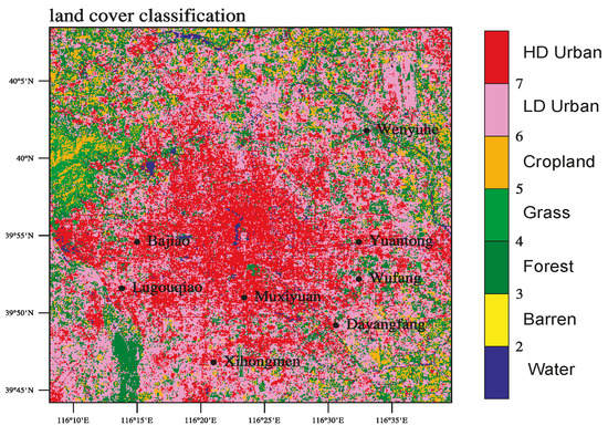
Figure 1.
Land cover classification of Beijing urban area and the locations of eight road sites.
2.2. Land Model
The IUM [17] as seen in the Supplementary Materials was used to perform the variational assimilation method. IUM was developed based on the common land model (CoLM) [30]. IUM integrates the land surface models for urban and natural land surfaces. For urban land surface, the anthropogenic heat release (AHR) was added in the energy balance equation as the radiation source term.
The surface energy balance for impervious land surface in IUM can be described as:
where is the specific heat capacity (J m−2 K−1); is the surface layer depth (m); is the impervious LST (K); is the timestep (s); is the thermal conductivity (W m−1 K−1); is the second layer soil temperature (K); is the ground heat flux (W m−2); is the surface net radiation (W m−2); is the sensible heat flux (W m−2); is the latent heat flux (W m−2); is the latent heat of evaporation for water or fusion for ice (J kg−1); is the impervious surface evaporation (mm s−1); and is the AHR (W m−2), it is associated with the LULC. The sensible heat flux is calculated as follows (Equation (2)):
where is the air density (kg m−3), is the specific heat for dry air (J kg−1 K−1), is the wind speed (m s−1), is the air potential temperature (K), and is the dimensionless bulk heat transfer coefficient. The impervious surface evaporation is parameterized as follows (Equation (3)):
where is the potential evaporation (m s−1), is the precipitation (mm/s), is the water drainage, is the impervious surface water depth (mm) in the previous time step, and is the impervious surface water depth (mm) in the current time step. can be parameterized as follows (Equation (4)):
where is the water density (kg m−3), which is approximately equal to 1000; is the aerodynamic resistance for evaporation (s m−1); is the specific humidity of the air (kg kg−1); and is the saturated specific humidity of the water surface (kg kg−1).
2.3. Data
We utilized the 1-h-resolution observations of the precipitation, wind speed and direction, near-surface relative air humidity and near-surface air temperature data from ROSATM (Vaisala Corporation: Vantaa, Finland) road weather stations manufactured by Vaisala Corporation to drive the IUM. The near-surface air pressure, downward solar radiation and downward longwave radiation data originated from the Global Land Data Assimilation System (GLDAS) [31]. The GLDAS data were interpolated temporally using the cubic spline method from 3 h to 1 h. The observed LST data from the road weather stations were used to initialize, assimilate and validate the IUM.
2.4. Variational Assimilation Method
In this paper, a variational approach was used to assimilate the impervious LST into the IUM, and the impervious surface energy balance equation (Equation (1)) was employed as the adjoint physical constraint. The variational assimilation approach assimilates the impervious LST through the adjustment of the tuned factor, that is the dimensionless bulk heat transfer coefficient under neutral conditions; which is related to the momentum roughness scale and the surface scaling length for heat flux, and not varied much during the assimilation period [32]. The tuned factor, i.e., the dimensionless bulk heat transfer coefficient under neutral conditions is calculated as follows (Equation (5)):
where is the dimensionless bulk heat transfer coefficient under neutral conditions, is the bulk Richardson number.
The corresponding cost function J is (Equation (6)):
where is the Lagrange multiplier, is the observed impervious LST (K), is the dimensionless bulk heat transfer coefficient under neutral conditions at the previous time step. , and are weight of the different terms, often defined as the inverse of the covariance matrix. This paper only tests the variational approach in several single-points sites. For the simplicity of the algorithm, these weights are all assumed to be constants. The flowchart of the integration of the variational assimilation method to IUM is nearly the same as Meng et al. 2009 [26].
The simulation time was from 10–24 August 2009. Two experiments were designed to compare the simulation result before and after assimilation for all the eight sites. For the control run, the observed LST was not assimilated into the IUM; while for the contrast run, the observed LSTs in each time-step were assimilated into the IUM. For Yuantong site, for the sake of the operational application, a third experiment (operational run) was designed which only assimilated the observed LST on 14:00 p.m. and 2:00 a.m.
3. Results and Discussions
First, we checked the site average diurnal cycle of the tuned factor for the control run (Figure 2a). The values of the tuned factor were between 0.00295 and 0.00334 and did not vary much during the assimilation window. So, it could be considered as an ideal tuned factor in the impervious LST assimilation.
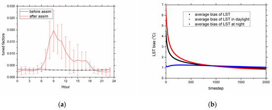
Figure 2.
(a) Site average diurnal cycles of the tuned factor before and after assimilation; (b) Site average convergence processes of the assimilation algorithm.
The site average convergence processes of the assimilation algorithm are shown in Figure 2b. The site average LST biases were reduced from about 7 k to 1 k in the daytime, and from 4.5 k to 1 k for the whole assimilation window. However, the LST biases were not nearly as varied at night because the tuned factor was associated with sensible heat flux (Figure 3), which was very low at night. Figure 2a also shows that after assimilation—in order to adjust the sensible heat flux and reduce the LST biases between the simulation and the observation—the site average diurnal cycle of the tuned factor changed drastically, especially in the daytime. As the tuned factors increased in the daytime, the sensible heat fluxes also increased (Figure 3a). As the result, the LSTs decreased (Figure 3b). The correlation coefficients between the LST differences and the sensible heat flux differences from the control run and the contrast run were −0.866 in the daytime and −0.352 at night, respectively.
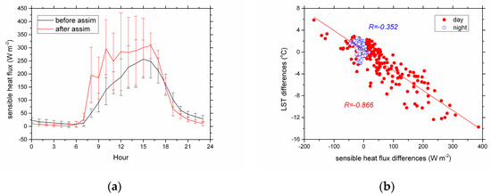
Figure 3.
(a) Site average diurnal cycle of the sensible heat flux before and after assimilation; (b) comparison of the site average sensible heat flux differences with the LST differences from the control run and contrast run.
Time series and diurnal cycles of the site average LST estimation from the control run and contrast run compared with the observation are shown in Figure 4. The biases, mean errors (MEs), root mean square errors (RMSEs) and correlation coefficients (Rs) are listed in Table 1. After assimilation, the simulated LSTs improved significantly. The bias decreased about 95%; the RMSE decreased about 74%; the R increased too. From Figure 4b, it was concluded that after assimilation, the simulated LSTs improved more in the daytime, especially from 10:00 to 19:00, because the sensible heat flux was relatively high in the daytime.
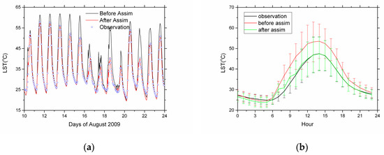
Figure 4.
(a) Time series and (b) diurnal cycles of the site average LST estimation from the control run and contrast run compared with the observation.

Table 1.
Biases, mean errors (MEs), root mean square errors (RMSEs) and correlation coefficients (Rs) of the site average LST estimate from the control run and contrast run compared with the observation.
Up to now, only the results in one circumstance have been discussed; that is, the observed impervious LST data in each time step that were assimilated into the IUM. For the sake of the application, a third experiment, namely the operational run, was designed. For the operational run, only the observed LST data at 14:00 and 02:00 were assimilated into the IUM. In the daytime, the tuned factors were considered the same as that on 14:00. At night, they were considered the same as that on 02:00. The Yuantong site was used to validate the assimilation method. Figure 5 is the diurnal cycles of the LST estimation from the control run, contrast run and operational run, compared with the observation for Yuantong site. The biases, mean errors (MEs), root mean square errors (RMSEs) and correlation coefficients (Rs) are listed in Table 2. Compared with the contrast run, the biases of the LST increased in the operational run, especially from 07:00 to 13:00; but the simulation results are still improved definitely compared with the control run. For the operational run, after assimilation, the bias decreased about 78%; the RMSE decreased about 31%.
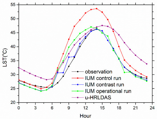
Figure 5.
Diurnal cycles of the LST estimate from the IUM from the control run, contrast run, operational run and u-HRLDAS compared with the observation for Yuantong site.
Table 2.
Biases, mean errors (MEs), root mean square errors (RMSEs) and correlation coefficients (Rs) of the LST estimate from the control run, contrast run, operational run and u-HRLDAS compared with the observation for Yuantong site.
To prove the advantage of the variational assimilation algorithm, the impervious LST simulation results from the urbanized high-resolution land data assimilation system (u-HRLDAS) [23], which is based on a single layer urban canopy model (Noah/SLUCM) [20], were compared with the simulation results of the IUM in Yuantong Site. Compared with the simulation results of u-HRLDAS, the simulation results of the operational run definitely improved. The bias decreased about 79%; the RMSE decreased about 24%.
4. Summary
In this paper, a variational assimilation method was developed and integrated into the IUM to improve the simulation of the impervious LST. A dimensionless bulk heat transfer coefficient under neutral conditions was used as the tuned factor to simplify the assimilation algorithm, which was related to the momentum roughness scale and the surface scaling length for heat flux and not varied much during the assimilation period.
The results indicate after the assimilation, the simulation of the impervious LST greatly improved. If the observed impervious LST data in every time were assimilated into the IUM, the bias of the impervious LST was reduced about 86 %. The simulated LST improved more in the daytime, especially from 10:00 to 19:00, as the sensible heat flux was relatively large in the daytime. For the operational run, the bias of the impervious LST was reduced about 78 %. Compared with the simulation results of u-HRLDAS, the simulation results of the operational run definitely improved. The bias decreased about 79%; the RMSE decreased about 24%.
In the near future, the variational assimilation method for impervious LST will be coupled with the variational assimilation method for LST in pervious land surfaces. A joint land data assimilation system will be developed based on the variational assimilation method of the soil moisture and the LST in both impervious and pervious land surfaces. The variational assimilation method for impervious LST will also be used to the road numerical forecast model to improve the forecast of road surface temperature.
Supplementary Materials
The following are available online at https://www.mdpi.com/2073-4433/11/4/380/s1. The codes of IUM were provided as the supplementary material.
Funding
This research was funded by the National Natural Science Foundation of China, Grant Number 41875125 and 41705086.
Acknowledgments
This work was supported by the National Natural Science Foundation of China under Grant 41875125. We thank Beijing Meteorological Bureau (www.bjmb.gov.cn) for the ROSATM road weather stations observational data; NASA for the GLDAS data (http://disc.sci.gsfc.nasa.gov/hydrology/data-holdings).
Conflicts of Interest
The author declares no conflict of interest.
References
- Gong, P.; Li, X.; Zhang, W. 40-Year (1978–2017) human settlement changes in China reflected by impervious surfaces from satellite remote sensing. Sci. Bull. 2019, 64, 756–763. [Google Scholar] [CrossRef]
- Zhou, L.; Dickinson, R.E.; Tian, Y.; Fang, J.Y.; Li, Q.X.; Robert, K.; Kaufmann, C.; Tucker, J.; Ranga, B. Evidence for a significant urbanization effect on climate in China. Proc. Natl. Acad. Sci. USA 2004, 101, 9540–9544. [Google Scholar] [CrossRef] [PubMed]
- Irwin, E.G.; Bockstael, N.E. The evolution of urban sprawl: Evidence of spatial heterogeneity and increasing land fragmentation. Proc. Natl. Acad. Sci. USA 2007, 104, 672–20677. [Google Scholar] [CrossRef] [PubMed]
- Grim, N.B.; Faeth, S.H.; Golubiewski, N.E.; Redman, C.L.; Wu, J.G. Global change and the ecology of cities. Science 2008, 319, 756–760. [Google Scholar] [CrossRef] [PubMed]
- Ma, Q.; He, C.; Wu, J.; Liu, Z.; Zhang, Q.F.; Sun, Z.X. Quantifying spatiotemporal patterns of urban impervious surfaces in China: An improved assessment using nighttime light data. Landsc. Urban Plan. 2014, 130, 36–49. [Google Scholar] [CrossRef]
- Ramamurthy, P.; Bou-Zeid, E. Contribution of impervious surfaces to urban evaporation. Water Resour. Res. 2014, 50, 2889–2902. [Google Scholar] [CrossRef]
- Xiao, R.; Ouyang, Z.; Zheng, H.; Li, W.F.; Schienke, E.; Wang, X.K. Spatial pattern of impervious surfaces and their impacts on land surface temperature in Beijing, China. J. Environ. Sci. China 2007, 19, 250–256. [Google Scholar] [CrossRef]
- Essa, W.; van der Kwast, J.; Verbeiren, B.; Batelaan, O. Downscaling of thermal images over urban areas using the land surface temperature-impervious percentage relationshop. Int. J. Appl. Earth Obs. 2013, 23, 95–108. [Google Scholar] [CrossRef]
- Hu, Y.; Jia, G.; Hou, M.; Zhang, X.X.; Zheng, F.X.; Liu, Y.H. The cumulative effects of urban expansion on land surface temperature in metropolitan Jingjintang China. J. Geophys. Res. 2015, 120, 9932–9943. [Google Scholar] [CrossRef]
- Wang, J.; Zhan, Q.; Guo, H.; Jin, Z.C. Characterizing the spatial dynamics of land surface temperature-impervious surface fraction relationshop. Int. J. Appl. Earth Obs. 2016, 45, 55–65. [Google Scholar] [CrossRef]
- Li, D.; Liao, W.; Rigden, A.J.; Liu, X.P.; Wang, D.G.; Malyshev, S. Urban heat island: Aerodynamics or imperviousness? Sci. Adv. 2019, 5, eaau4299. [Google Scholar] [CrossRef]
- Kalnay, E.; Cai, M. Impact of urbanization and land-use change on climate. Nature 2003, 423, 528–531. [Google Scholar] [CrossRef]
- Ren, G.; Zhou, Y.; Chu, Z.; Zhou, J.X.; Zhang, A.Y.; Guo, J.; Liu, X.F. Urbanization effects on observed surface air temperature trends in north China. J. Clim. 2008, 21, 1333–1348. [Google Scholar] [CrossRef]
- Meng, C. A numerical forecast model for road meteorology. Meteorol. Atmos. Phys. 2018, 130, 485–498. [Google Scholar] [CrossRef]
- Best, M.J.; Grimmond, C.S.B. Key Conclusions of the First International Urban Land Surface Model Comparison Project. Bull. Am. Meteorol. Soc. 2015, 96, 805–819. [Google Scholar] [CrossRef]
- Liu, Y.; Chen, F.; Warner, T.; Basara, J. Verification of a mesoscale data-assimilation and forecasting system for the Okalahoma city area during the joint urban 2003 field project. J. Appl. Meteorol. Clim. 2006, 45, 912–929. [Google Scholar] [CrossRef]
- Meng, C. The integrated urban land model. J. Adv. Model. Earth Syst. 2015, 7, 759–773. [Google Scholar] [CrossRef]
- Wouters, H.; Demuzere, M.; Blahak, U.; Keith, W.; Gordon, B. The efficient urban canopy dependency parameterization (SURY) v1.0 for atmospheric modelling: Description and application with the COSMO-CLM model for a Belgian summer. Geosci. Model Dev. 2016, 9, 3027–3054. [Google Scholar] [CrossRef]
- Masson, V. A physically-based scheme for the urban energy budget in atmospheric models. Bound. Layer Meteorol. 2000, 94, 357–397. [Google Scholar] [CrossRef]
- Kusaka, H.; Kondo, H.; Kikegawa, Y.; Kimura, F. A simple single-layer urban canopymodel for atmospheric models: Comparison with multi-layer and slab models. Bound. Layer Meteorol. 2001, 101, 329–358. [Google Scholar] [CrossRef]
- Martilli, A.; Clappier, A.; Rotach, M.W. An urban surface exchange parameterization for mesoscale models. Bound. Layer Meteorol. 2002, 104, 261–304. [Google Scholar] [CrossRef]
- Oleson, K.W.; Bonan, G.B.; Feddema, J.; Vertenstein, M.; Grimmond, C.S.B. An urban parameterization for a global climate model. Part I: Formulation and evaluation for two cities. J. Appl. Meteorol. Clim. 2008, 47, 1038–1060. [Google Scholar] [CrossRef]
- Chen, F.; Manning, K.W.; LeMone, M.A.; Trier, S.B.; Alfieri, J.G.; Roberts, R.D.; Blanken, P.D. Description and evaluation of the characteristics of the NCAR high-resolution land data assimilation system. J. Appl. Meteorol. Clim. 2007, 46, 694–713. [Google Scholar] [CrossRef]
- Castelli, F.; Entekhabi, D.; Caporali, E. Estimation of surface heat flux and an index of soil moisture using adjoint-state surface energy balance. Water Resour. Res. 1999, 35, 3115–3125. [Google Scholar] [CrossRef]
- Caparrini, F.; Castelli, F.; Entekhabi, D. Variational estimation of soil and vegetation turbulent transfer and heat flux parameters from sequences of multisensor imagery. Water Resour. Res. 2004, 40, W12515. [Google Scholar] [CrossRef]
- Meng, C.; Li, Z.; Zhan, X.; Shi, J.C.; Liu, C.Y. Land surface temperature data assimilation and its impact on evapotranspiration estimates from the Common Land Model. Water Resour. Res. 2009, 45, W02421. [Google Scholar] [CrossRef]
- Bateni, S.M.; Entekhabi, D.; Jeng, D.S. Variational assimilation of land surface temperature and the estimation of surface energy balance components. J. Hydrol. 2013, 481, 143–156. [Google Scholar] [CrossRef]
- Meng, C.; Zhang, C.; Tang, R. Variational estimation of land-atmosphere heat fluxes and land surface parameters using MODIS remote sensing data. J. Hydrometeorol. 2013, 14, 608–621. [Google Scholar] [CrossRef]
- Xu, T.; He, X.; Bateni, S.M.; Auligne, T.; Liu, S.; Xu, Z.W.; Zhou, J.; Mao, K. Mapping regional turbulent heat fluxes via variational assimilation of land surface temperature data from polar orbiting satellites. Remote Sens. Environ. 2019, 221, 444–461. [Google Scholar] [CrossRef]
- Dai, Y.; Zeng, X.; Dickinson, R.E.; Baker, I.; Bonan, G.; Bosilovich, M.; Denning, S.; Dirmeyer, P.; Houser, P.; Niu, G. The common land model. Bull. Am. Meteorol. Soc. 2003, 84, 1013–1023. [Google Scholar] [CrossRef]
- Rodell, M.; Houser, P.R.; Jambor, U.; Gottschalck, K.; Mitchell, C.-J.; Meng, K.; Arsenault, B.; Cosogrove, J.; Radakovich, M.; Entin, J. The global land data assimilation system. Bull. Am. Meteorol. Soc. 2004, 85, 381–394. [Google Scholar] [CrossRef]
- Caparrini, F.; Castelli, F.; Entekhabi, D. Mapping of land-atmosphere heat fluxes and surface parameters with remote sensing data. Bound. Layer Meteorol. 2003, 107, 605–633. [Google Scholar] [CrossRef]


© 2020 by the author. Licensee MDPI, Basel, Switzerland. This article is an open access article distributed under the terms and conditions of the Creative Commons Attribution (CC BY) license (http://creativecommons.org/licenses/by/4.0/).