Characteristics of Decaying Convective Boundary Layers Revealed by Large-Eddy Simulations

Abstract

The decay of the Convective Boundary Layer (CBL) is studied using large-eddy simulations of free and advective CBLs, in which surface heat supply is suddenly cut off. After the cutoff, coherent convective circulations last about one convective time scale and then fade away. In the mixed layer, the decay time scale increases with height, indicating that nonlocal eddies decay slower than near-surface local eddies. The slower decay of turbulence in the middle of CBL than near-surface turbulence is reconfirmed from the analysis of pattern correlations of perturbations of vertical velocity. Perturbations of potential temperature and scalar concentration decay faster and slower than vertical velocity perturbations, respectively. A downward propagation of negative heat flux and its oscillation are found and a quadrant analysis reveals that warmer air sinking events are responsible for the downward propagation. The fourth quadrant events seem to be induced by demixing of air parcels, entrained from above the CBL. The advective CBL simulation with geostrophic wind illustrates that near-surface eddies are mechanically generated and they decelerate flow from the bottom up in the CBL/residual layer. The two-dimensional spectra show the height- and scale-dependent characteristics of decaying convective turbulence again in the free and advective boundary layer simulations.

1. Introduction

The Planetary Boundary Layer (PBL), the bottom layer of the troposphere in contact with the Earth’s surface, responds to surface forcings “with a timescale of about an hour or less” and thus has a strong diurnal cycle over land [1]. Heating of land surface by solar radiation generates convective turbulence and a Convective (planetary) Boundary Layer (CBL) develops with local and nonlocal mixing in the surface and mixed layer and top entrainment in the entrainment zone. Convective turbulence decays near sunset, and the mixed layer is transitioned to a residual layer and a shallow stable boundary layer starts to develop near the surface. During this so-called evening transition, occurrences of surface temperature drop, specific humidity jump, and abrupt wind speed decay are reported [2]. However, these kinds of variations are still poorly predicted [3].

The decay of convective turbulence was investigated through laboratory experiments [4], observations [2,5,6,7,8,9], and numerical simulations [10,11,12,13,14,15,16]. Sorbjan [11] simulated a decaying CBL using a Large-Eddy Simulation (LES) model. He considered gradually decreasing surface heat flux over time and showed that the decay of Turbulent Kinetic Energy (TKE) is governed by two time scales, the external time scale of the surface heat flux change, and the convective time scale $t_{\ast }=z_i/w_{\ast }$ where $z_i$ and $w_{\ast }$ are, respectively, the inversion height and the convective velocity scale [17]. He also found that large eddies persist even when the surface heat flux becomes negative. Recently, Darbieu et al. [15] simulated a more realistic decay of CBL using an LES model and the Boundary Layer Late Afternoon and Sunset Turbulence (BLLAST) field experiment data. Based on the LES and observation data, they found two phases in which TKE decays slowly and quickly, respectively. The changes in TKE decay occur first in the upper PBL and the vertical wind spectral shape changes more with increasing height in the PBL. The transitional turbulence decay can also be implicitly simulated using a single-column modeling technique but the simulation is sensitive to the details of parameterization (e.g., the profile of eddy diffusivity) [14]. The recent evaluation by Couvreux et al. [16] shows that the operational models are able to reproduce the temporal and spatial variability of boundary layer depth and other variables but some systematic biases of temperature and humidity still exist. Instead of gradually decaying CBLs, Nieuwstadt and Brost [10] performed idealized CBL simulations in which surface sensible heat flux is suddenly stopped. They found that the decay of convective turbulence scales with $t_{\ast }$. While the temperature fluctuations decay almost immediately after the flux is stopped, the TKE stays constant for a period of $\sim t_{\ast }$. In their simulations, vertical velocity fluctuations decay faster than horizontal velocity fluctuations. They also provided some evidence of a decoupling of large and small scales during the decay. Pino et al. [12] investigated the role of wind shear and inversion strength on the decay of similar CBLs. The length scale of vertical velocity fluctuations remains nearly constant but the length scales of other variables increase over time after surface heat flux is stopped. They showed that convective turbulence with shear decays slower than purely buoyancy-driven convective turbulence but inversion strength is less influential. They insisted that the faster dissipation of small-scale eddies induces “demixing” of entrained air parcels and an oscillation of vertical heat flux. However, the relationship between the demixing and the oscillating heat flux is not sufficiently understood yet. In addition, the decoupling of large- and small-scale eddies needs to be investigated in more detail.

In this study, we design two numerical experiments in which the upward surface sensible heat flux is suddenly stopped as those in Nieuwstadt and Brost [10] and Pino et al. [12]. Growing and decaying phases of a purely convective boundary layer and an advective convective boundary layer, being advected following geostrophic wind, are simulated. We demonstrate more detailed features of decaying convective turbulence, and demixing and decoupling are studied in a different perspective. The LES model used in this study and its setup are described in Section 2. We present and discuss the simulation results in Section 3. A summary and conclusions are given in Section 4.

2. Model Description and Setup

We use the PArallelized LES Model (PALM) version 6.0 [18] to simulate developing and suddenly decaying CBLs. LES models resolve eddies of interest explicitly and parameterize subfilter-scale eddies based on the inertial subrange theory, and thus energy-containing eddies (e.g., boundary layer thermals) can be efficiently simulated without resolving less important smaller eddies [19]. The model that we used is based on the implicitly filtered Navier-Stokes equations in Boussinesq-approximated form and it solves six prognostic variables, velocity components u, v, w, potential temperature $\theta$, passive scalar concentration s, and subgrid-scale TKE $e_s$ on the staggered Arakawa C-grid [20]. A third-order Runge-Kutta scheme [21] is used for time integration and an upwind-biased 5th-order scheme [22] is used for discretizing advection terms. Subgrid-scale fluxes are parameterized using the 1.5-order Deardorff [23] scheme.

Two experiments with zero wind and geostrophic wind ($u_g,v_g$) = (10, 0 m ${\mathrm{s}}^{-1}$), respectively, are performed to investigate free and advective CBLs. Each experiment is simulated with a constant surface sensible heat flux 0.1 K m ${\mathrm{s}}^{-1}$ for three hours and then simulated without surface heat supply for three more hours. The passive scalar flux is 1 g m ${\mathrm{s}}^{-1}$ until the cutoff time of heat flux $t_c$ (t = 3 h) and 0 g m ${\mathrm{s}}^{-1}$ afterwards following the heat flux setup. The grid size in the x (streamwise) and y (spanwise) directions is 20 m and the grid size in the z (vertical) direction is 20 m below z = 1.2 km and gradually stretched to 50 m above that level. The computation domain with $512\times 512\times 80$ grid boxes covers $10.24\times 10.24\times 2.07$ k${\mathrm{m}}^3$. Rayleigh damping is implemented above z = 1.7 km to damp gravity waves reflected at the top boundary. Each experiment starts with a simple temperature sounding, in which $\theta$ is 300 K below z = 0.7 km and increases with a lapse rate of 10 K k${\mathrm{m}}^{-1}$ above z = 0.7 km. The Coriolis force is ignored to make the experiments as simple as possible. In the PALM, the time step is automatically determined to satisfy the Courant-Friedrichs-Lewy criterion and it ranges from 3.3 s to 20 s. The simulation data for the last three hours are sampled every ∼60 s but the sampling interval fluctuates by several seconds due to the temporally varying time step.

3. Results and Discussion

3.1. Free Decaying Convective Boundary Layer

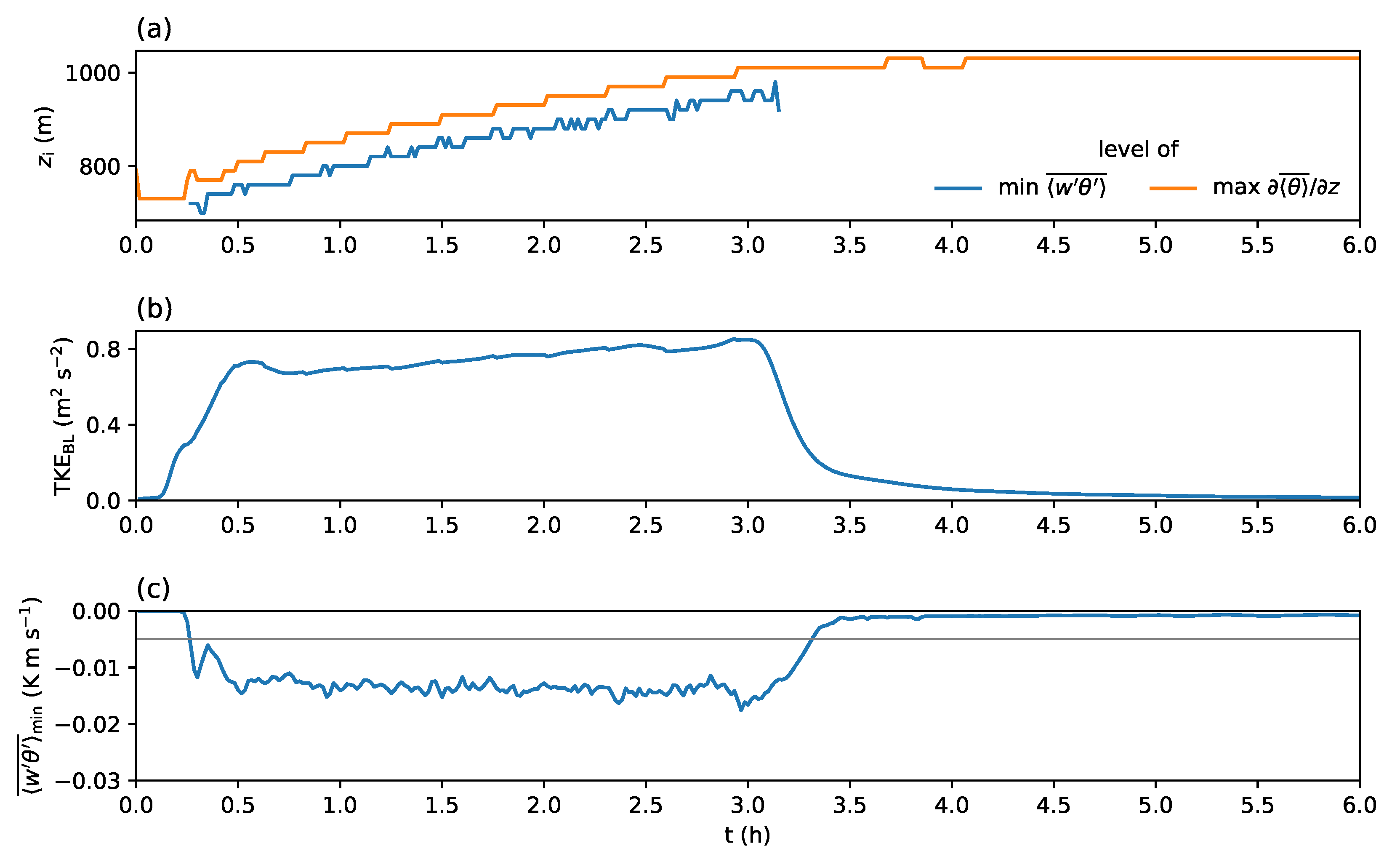
The simulation without backgound wind shows developing and decaying phases of the free CBL and its transition to a residual layer. To illustrate the PBL depth and its time evolution, we calculate the inversion height $z_i$, defined as the level of minimum sensible heat flux, and the level of maximum vertical gradient of potential temperature $z_{ig}$ (Figure 1a) [24]. The periods when the magnitude of minimum heat flux is smaller than 0.005 K m ${\mathrm{s}}^{-1}$ and when the maximum heat flux is negative are excluded from the calculation of $z_i$. The inversion height increases until $t=t_c$ and then stays almost constant for ∼540 s. Then, the heat flux becomes negative at all the vertical levels (see later discussions and Figure 5c), implying that the vertical structure of CBL is broken. The time interval between $t_c$ and the CBL breakage is comparable to $t_{\ast }$ (648 s at $t=t_c$). The level $z_{ig}$ starts from around the bottom of initial capping inversion (0.7 km) and increases to 1010 m at t = $t_c$, and then it is almost constant even after the CBL breakage. Note that $z_{ig}$ is higher than $z_i$ by 30–70 m because of their different definitions [24]. Actually, $z_{ig}$ represents the entrainment interface, irrespective of heat flux profile below, and it is close to the top of entrainment zone or the top of residual layer while $z_i$ is usually located in the middle of the entrainment zone. Figure 1b shows the time series of the TKE averaged below $z_{ig}$. After 45-min spinup, the vertically averaged TKE increases slowly until t = $t_c$, followed by its abrupt decrease after ∼200 s. The time evolution of the minimum heat flux is presented in Figure 1c. The minimum heat flux represents the strength of top entrainment, proportional to the activity of overshooting thermals and downward heat transport [24]. After the spinup, its magnitude increases slightly until t = $t_c$ and then decreases immediately.

Figure 2 shows the vertical velocity fields at $t=t_c$ and z = 40, 460 ($\sim z_i/2$), and 940 m ($z_i$) and the same fields 604, 1204, and 3603 s after $t_c$. Convection cells with narrow branches of near-surface updrafts, downdrafts and narrow circumferential updrafts in the mixed layer, so-called cellular convection, and overshooting thermals (or updrafts) across the entrainment zone are clearly visible at $t=t_c$ (Figure 2a,e,i). Turbulent eddies seem to decay quickly from the bottom up. For example, the narrow branches of updrafts near the surface become weak and broad within a period of $\sim t_{\ast }$ (Figure 2i,j). The number of overshooting updrafts decreases, too, corresponding to the decrease of minimum heat flux after $t=t_c$ (Figure 1c). In contrast, the cellular up- and downdrafts in the middle of CBL maintain their strength and position for more than 604 s. For example, updrafts on the rising branches are still faster than 1 m ${\mathrm{s}}^{-1}$ at $t=t_c$ + 604 s. This illustrates that boundary layer thermals survive for a time period in the order of $t_{\ast }$ whereas near-surface eddies decay quickly. The cellular up- and downdrafts decay and overshooting updrafts disappear completely afterwards. One hour after $t=t_c$, the up- and downdrafts become much weaker than before and they lost their cellular structure at z = $\sim z_i/2$, now in the residual layer.

The vertical velocity fields in the y-z plane (Figure 3) and the potential temperature fields in the same y-z plane (Figure 4) illustrate the vertical structure of decaying convection cells. While the near-surface updrafts decay quickly, the convection cells seem to survive longer. At the initial decaying phase, the individual updrafts of the cells become weak but diffused, filling gaps between updrafts and making wider convection cells (Figure 3b,c). During the decay, small downdrafts penetrate down through cellular updrafts but convective circulation and diffusing motions seem to maintain the boundary layer circulations until $t=t_c$ + 905 s. The large convection cells, however, break into smaller eddies 1202 s after $t=t_c$ (Figure 3e). The black contours of 301.51 K potential temperature in Figure 3c–g illustrate thermal stratification in the middle of PBL briefly, e.g., the air below and above the contours are cooler and warmer than 301.51 K, respectively, as can be confirmed in Figure 4. The value of 301.51 K is selected to visualize the thermal stratification as best as possible. Cellular up- and downdrafts are shown to be located in cooler and warmer regions, respectively, at $t-t_c$ = 604, 905, and 1202 s (Figure 3c–e). Thus, updrafts push cool air upward and downdrafts drag warm air downward during the decay. The potential temperature fields in Figure 4 confirms that cellular up- and downdrafts stack cooler and warmer air, respectively, inducing the undulating distribution of potential temperature at $t-t_c$ = 604, 905, and 1202 s. This kind of undulating distribution appears several hundred seconds more but becomes less and less distinct over time (not shown). Along with the boundary layer scale circulations, local downdrafts touch the bottom surface as the cold pools from deep convective clouds do [25], but they are not spreading out at the bottom surface because they are warmer than near-surface air (not shown). This kind of abnormal and unsustainable circulations weaken gradually with the contours getting flatter over time. Eddies, with scales of several hundred meters, still exist ∼1 h after $t=t_c$ but they disappear completely two more hours later with a stably stratified residual layer (Figure 3f,g).

The vertical structure of the decaying CBL is presented in the time series of vertical profiles of TKE, vertical velocity variance $\overline{\langle {w^{\prime }}^2\rangle }$, and vertical heat flux $\overline{\langle {\theta }^{\prime }{w}^{\prime }\rangle }$ (Figure 5). In this study, overbars and angle brackets denote temporal (60 s) and horizontal averages and primes denote perturbations from the horizontal averages. The TKE in the mixed layer maintains the initial level for several hundred seconds, for example, TKE at $z=z_i/2$ lost 5% in 360 s, and then decays from the bottom up. The e-folding decay time of TKE also increases with height, confirming the bottom-up decay. The variance of vertical velocity, representing vertical turbulence, is larger in the middle of CBL than near the surface or the CBL top. The e-folding decay time increases with height, too, but it is shorter than that of TKE especially near the surface. This indicates that the near-surface TKE is maintained by horizontal diverging and converging motions induced by subsiding downdrafts. The profiles of vertical heat flux illustrate that the vertical thermal structure of CBL, positive and negative heat flux in and above the mixed layer, is maintained until $t=t_c$ + 540 s, then negative heat flux propagates down to the bottom. After the negative heat flux dominates throughout the boundary layer, an oscillation of heat flux occurs despite of its small amplitude. This downward propagation and the following oscillation were simulated in previous numerical studies [10,12] and observed in the real atmosphere [5,7]. These are known to be induced by demixing of air parcels, entrained from above the PBL top, and their returning to equilibrium levels [12]. The e-folding time of vertical heat flux increases vertically in the mixed layer but the time scale is shorter than that of TKE. This is attributable to that potential temperature perturbations decay faster than velocity perturbations [10].

The downward propagating negative heat flux and the following heat flux oscillation have been explained by circulations of demixed (or non-mixed) air parcels after small-scale turbulence decays [10,12] but the explanation has not been proven yet. For this, a quadrant analysis of ${\theta }^{\prime }$ and $w^{\prime }$ is done (Figure 6). Perturbations at every grid point and every ∼60 s are classified into the four quadrants—warm air rising, cool air rising, cool air sinking, and warm air sinking events—and the classified events are averaged to show the contribution of the individual quadrants to vertical heat transport [24,26]. The first and third quadrants represent the contributions by rising thermals and subsidence, respectively. They are the main upward heat transporters in the mixed layer. The other two quadrants do a minor role in the mixed layer, but they are important in the entrainment zone. Overshooting thermals become cooler than the stably stratified environment and thus their contribution to downward heat flux is represented by the second quadrant, cool air rising. The fourth quadrant, representing warm air sinking events, is weaker than the second quadrant not only in the entrainment zone but also in the lower mixed layer. However, the contribution by the fourth quadrant events, especially in the lower mixed layer, becomes stronger several hundred seconds after $t=t_c$. Thus, warm air sinking events appear to induce the downward propagation of negative heat flux. After the cutoff of surface heat flux, near-surface air is a little cooler than previously heated and already lifted air and thus the lower mixed layer becomes weakly stable. We speculate that demixed downdrafts from the entrainment zone or from the middle of CBL are now warmer than the environment (Figure 3c–e) and they contribute to the downward propagating negative heat flux. However, the histories of demixed downdrafts are still questionable and a more sophisticated method (e.g., a Lagrangian tracking) is required to reveal the mechanism of this downward propagation completely.

Time series of the pattern correlation between the perturbations at $t=t_c$ and later perturbations illustrate the decaying characteristics in a different perspective (Figure 7). This kind of analysis is meaningful only for the free CBL because convection cells develop and decay nearly at the same place. The pattern correlation of the vertical velocity shows that convective turbulence in the middle of CBL decays slower than that near the surface or at the CBL top, as the vertical velocity variance decays (Figure 5b). The pattern correlation at $z=z_i/2$, for instance, is higher than 0.4 at 600 s ($\sim t_{\ast }$) after $t=t_c$. The pattern correlation of potential temperature decreases more quickly than that of vertical velocity. In contrast to potential temperature, the pattern correlation of passive scalar concentration decreases slower than that of vertical velocity, implying that passive scalar has a longer memory. It is also notable that the pattern correlation of passive scalar has maximum peaks at higher levels than that of vertical velocity. This may be due to the fact that scalar perturbations have less resistance (or more inertia) in the entrainment zone than thermal and momentum perturbations, but this needs a further investigation.

To demonstrate the height- and scale-dependent characteristics of convective turbulence, two-dimensional spectra of vertical velocity and potential temperature near the surface and at the middle of CBL are calculated and plotted in Figure 8. In this study, Fourier coefficients in a two-dimensional wavenumber space are calculated first, and then the radial averages of the coefficients are computed. While one-dimensional spectra can show only one directional spectral energy, this kind of two-dimensional spectra can represent spectral energy in all horizontal directions, thus illustrating spectral energy of convection cells better than its one-dimensional counterpart. The spectra of vertical velocity have maximum peaks in the wavelength range of 1280–2560 m and monotonically decrease with increasing frequency (decreasing wavelength) at the middle of CBL (Figure 8b). The spectra near the surface are flat in the wavelength range of 320–1280 m with cascading in the smaller wavelength range (Figure 8a). The flat spectral range is attributed to the near-surface local eddies and the near-surface spectral energy decays quickly shortly after the surface heat flux is stopped. In contrast to the fast decay near the surface, the spectrum of vertical velocity at the middle of CBL changes very little for the initial 362 s. This demonstrates that nonlocal eddies are active for the initial several hundred seconds. Then, the nonlocal eddies decay over time along with the decaying near-surface local eddies. The spectral energy of potential temperature near the surface decays quickly over time (Figure 8c). For example, the sum of spectral energies (=variance) of potential temperature decreases by a factor of 67.2 for the initial 362 s. At the middle of CBL, the spectral energy of potential temperature decays more slowly than that near the surface, too (Figure 8d).

3.2. Advective Decaying Convective Boundary Layer

The simulation of advective decaying CBL reveals the role of mechanically generated eddies near the surface. Figure 9 shows vertical velocity fields in the y-z plane, illustrating the vertical structure of convective rolls. Convective rolls, pairs of linearly aligned and circulating up- and downdrafts, are being advected in the streamwise direction during their developing and decaying phases and thus tracking of individual rolls is difficult at a fixed position. Nonetheless, decaying characteristics in this advective CBL are identifiable in the series of vertical velocity fields in the fixed y-z plane (Figure 9) and the characteristics are similar to those in the free CBL. For example, convective rolls become weak but a little wider and then break into much smaller eddies (Figure 9a–e). The abnormal circulations observed in Figure 3, in which cool air rises and warm air sinks, are less distinct in this advective CBL. Moreover, up- and downdrafts in the convective rolls seem to decay more slowly than those in the free CBL. It is also notable that local eddies are generated constantly near the surface even after nonlocal eddies disappear and they survive until the end of the 6-h simulation. However, in the absence of surface cooling and strong stratification, the surface eddies grow up to several hundred meters, thus the eddies do not seem to be local at the end of the simulation.

The potential temperature fields in Figure 10 confirm that the undulating potential temperature distribution in the free decaying CBL (Figure 4) is not very distinct in the advective decaying CBL. It is also remarkable that the regions cooler than 301.4 K in the advective decaying CBL are wider than those in the free decaying CBL. Another remarkable feature is that potential temperature at the end of the simulation seems to be less stratified than in the free decaying CBL (Figure 10g) due to the more active near-surface eddies in the advective decaying CBL (Figure 9g).

The time series of vertical profiles of TKE, vertical velocity variance, vertical heat flux, vertical momentum flux $\overline{\langle u^{\prime }{w}^{\prime }\rangle }$, and horizontally and temporally averaged streamwise velocity $\overline{\langle u\rangle }$ are plotted in Figure 11. While the vertical velocity variance and the heat flux decay from the bottom up as in the free decaying CBL (Figure 5b,c), near-surface TKE is higher and decays slower than TKE in the middle of CBL (Figure 11a). This slower decay is attributable to the near-surface eddies such as sweeps and ejections interacting with the convective rolls (not shown). Note that the e-folding times of TKE, vertical velocity variance, and vertical heat flux in this advective CBL are longer than those in the free convective boundary layer, as shown by the black and gray dots in Figure 11. For instance, the e-folding time of TKE at $z=z_i/2$ is 1261 s in the advective CBL and it is 966 s in the free CBL. We speculate that surface wind shear induces more lasting vertical circulations. Momentum flux decays quickly, too, except near the surface. Downward momentum flux is maintained to a certain degree and the vertical range of negative momentum flux extends upward over time (Figure 11d). This is consistent with the upward growth of the surface eddies seen in Figure 9. As a result, mean flow in the lower CBL or in the lower residual layer (after the CBL breakage) is decelerated over time until the end of the simulation (Figure 11e). In the real atmosphere, however, the growth of the surface eddies is more suppressed in the shallow and stable boundary layer over the radiatively cooled surface.

Two-dimensional spectra of vertical velocity and streamwise velocity in the advective CBL are presented in Figure 12. Near the surface and in the wavelength range of 320–1280 m, the spectra of vertical velocity are quite flat for the initial 181 s but large eddies decay faster than small eddies, and parabolic spectra of vertical velocity are left finally (Figure 12a). The wavelength of the spectral peak ranges between 160 and 320 m, matching with the scale of the near-surface eddies (Figure 9). The spectrum of vertical velocity at the middle of CBL stays almost the same for the initial 361 s as in the free CBL. Since then, the spectra decrease and the gap between two successive spectra becomes narrower over time than the gap in the free CBL (Figure 8b), indicating the slower decay in the advective CBL. The slower decay, distinct in the wavelengths smaller than 640 m, is related to the surface eddies growing up to several hundred meters (Figure 9g). The spectra of streamwise velocity near the surface and in the wavelengths smaller than 320 m decay very slowly for the three hours after $t=t_c$ but the spectra of larger eddies decay faster as the spectra of vertical velocity (Figure 12a,c). At the middle of CBL, the spectral energies of streamwise velocity stay almost the same for the initial 721 s and then decay but the impact of the surface eddies is hardly detectable (Figure 12d).

4. Summary and Conclusions

The characteristics of free and advective decaying CBLs were investigated using an LES model. After surface sensible heat supply is suddenly cut off, coherent circulations such as convection cells and convective rolls last for a period comparable to the convective time scale and then fade away, as the decay of volume-averaged TKE in the previous studies [10,12]. Whereas Nieuwstadt and Brost [10] reported that the decay rate of convective turbulence is the same at all heights, the height dependency of the decay rate is found in this study. For instance, the decay time scale of TKE increases with height in the mixed layer because nonlocal eddies decay slower than near-surface local eddies. Pattern correlation analysis demonstrates that nonlocal eddies survive longer than local eddies and temperature (passive scalar) perturbations decay faster (slower) than momentum perturbations. The downward propagation of negative heat flux is shown to be related to warmer air sinking quadrant events, and the fourth quadrant events may be induced by demixing of air parcels, entrained from above the CBL. The height- and scale-dependent decaying characteristics are reconfirmed in the two-dimensional spectra. In the advective decaying boundary layer, surface wind shear generates long-lasting local eddies and they grow over time, decelerating mean flow in the lower mixed layer and in the lower residual layer. The surface wind shear acts to prolong the decay time scale by generating local eddies near the surface, and this can explain the slower decay of turbulence in the advective decaying CBL in Pino et al. [12].

We demonstrated the characteristics of decaying convective boundary layers in many perspectives. Even in these idealized decaying CBLs, convective turbulence decays differently with time and space. Recently, van Heerwaarden and Mellado [27] showed that the CBL grows and decays simultaneously over the surface with a constant temperature. Thus, convective turbulence actually develops and decays simultaneously but differently with time and space. A challenge is to understand the role of coherent structures in the localized developing and decaying phases. We need a more sophisticated method to identify and track individual coherent structures, as done for shallow cumulus clouds [28]. Then, we can understand more about the time-varying features of PBL and this will help us refine PBL parameterization schemes (e.g., predicting the transitional decrease of TKE more precisely).

References

1. Stull, R.B. An Introduction to Boundary Layer Meteorology; Springer: Dordrecht, The Netherlands, 1988. [Google Scholar] [CrossRef]
2. Acevedo, O.C.; Fitzjarrald, D.R. The early evening surface-layer transition: Temporal and spatial variability. J. Atmos. Sci. 2001, 58, 2650–2667. [Google Scholar] [CrossRef]
3. Svensson, G.; Holtslag, A.A.; Kumar, V.; Mauritsen, T.; Steeneveld, G.J.; Angevine, W.M.; Bazile, E.; Beljaars, A.; de Bruijn, E.I.; Cheng, A.; et al. Evaluation of the diurnal cycle in the atmospheric boundary layer over land as represented by a variety of single-column models: The second GABLS experiment. Bound. Layer Meteorol. 2011, 140, 177–206. [Google Scholar] [CrossRef] [Green Version]
4. Cole, G.S.; Fernando, H.J. Some aspects of the decay of convective turbulence. Fluid Dyn. Res. 1998, 23, 161–176. [Google Scholar] [CrossRef]
5. Caughey, S.J.; Kaimal, J.C. Vertical heat flux in the convective boundary layer. Q. J. R. Meteorol. Soc. 1977, 103, 811–815. [Google Scholar] [CrossRef]
6. Grant, A.L. An observational study of the evening transition boundary-layer. Q. J. R. Meteorol. Soc. 1997, 123, 657–677. [Google Scholar] [CrossRef]
7. Grimsdell, A.W.; Angevine, W.M. Observations of the afternoon transition of the convective boundary layer. J. Appl. Meteorol. 2002, 41, 3–11. [Google Scholar] [CrossRef]
8. Fitzjarrald, D.R.; Freedman, J.M.; Czikowsky, M.J.; Sakai, R.K.; Acevedo, O.C.; Moraes, O.L. Momentum and scalar transport during the decay of CBL turbulence. In Proceedings of the 16th AMS Symposium on Boundary Layers and Turbulence, Portland, ME, USA, 8–13 August 2004; pp. 187–189. [Google Scholar]
9. Lothon, M.; Lohou, F.; Pino, D.; Couvreux, F.; Pardyjak, E.R.; Reuder, J.; Vilà-Guerau de Arellano, J.; Durand, P.; Hartogensis, O.; Legain, D.; et al. The BLLAST field experiment: Boundary-Layer Late Afternoon and Sunset Turbulence. Atmos. Chem. Phys. 2014, 14, 10931–10960. [Google Scholar] [CrossRef] [Green Version]
10. Nieuwstadt, F.T.; Brost, R.A. The decay of convective turbulence. J. Atmos. Sci. 1986, 43, 532–546. [Google Scholar] [CrossRef] [Green Version]
11. Sorbjan, Z. Decay of convective turbulence revisited. Bound. Layer Meteorol. 1997, 82, 501–515. [Google Scholar] [CrossRef]
12. Pino, D.; Jonker, H.J.; Vilà-Guerau de Arellano, J.; Dosio, A. Role of shear and the inversion strength during sunset turbulence over land: Characteristic length scales. Bound. Layer Meteorol. 2006, 121, 537–556. [Google Scholar] [CrossRef]
13. Beare, R.J.; Edwards, J.M.; Lapworth, A.J. Simulation of the observed evening transition and nocturnal boundary layers: Large-eddy simulation. Q. J. R. Meteorol. Soc. 2006, 132, 81–99. [Google Scholar] [CrossRef]
14. Edwards, J.M.; Beare, R.J.; Lapworth, A.J. Simulation of the observed evening transition and nocturnal boundary layers: Single-column modelling. Q. J. R. Meteorol. Soc. 2006, 132, 61–80. [Google Scholar] [CrossRef]
15. Darbieu, C.; Lohou, F.; Lothon, M.; Vilà-Guerau de Arellano, J.; Couvreux, F.; Durand, P.; Pino, D.; Patton, E.G.; Nilsson, E.; Blay-Carreras, E.; et al. Turbulence vertical structure of the boundary layer during the afternoon transition. Atmos. Chem. Phys. 2015, 15, 10071–10086. [Google Scholar] [CrossRef] [Green Version]
16. Couvreux, F.; Bazile, E.; Canut, G.; Seity, Y.; Lothon, M.; Lohou, F.; Guichard, F.; Nilsson, E. Boundary-layer turbulent processes and mesoscale variability represented by numerical weather prediction models during the BLLAST campaign. Atmos. Chem. Phys. 2016, 16, 8983–9002. [Google Scholar] [CrossRef] [Green Version]
17. Deardorff, J.W. Convective velocity and temperature scales for the unstable planetary boundary layer and for Rayleigh convection. J. Atmos. Sci. 1970, 27, 1211–1213. [Google Scholar] [CrossRef] [Green Version]
18. Maronga, B.; Gryschka, M.; Heinze, R.; Hoffmann, F.; Kanani-Sühring, F.; Keck, M.; Ketelsen, K.; Letzel, M.O.; Sühring, M.; Raasch, S. The Parallelized Large-Eddy Simulation Model (PALM) version 4.0 for atmospheric and oceanic flows: Model formulation, recent developments, and future perspectives. Geosci. Model Dev. 2015, 8, 2515–2551. [Google Scholar] [CrossRef] [Green Version]
19. Moeng, C.H.; Sullivan, P.P. A comparison of shear- and buoyancy-driven planetary boundary layer flows. J. Atmos. Sci. 1994, 51, 999–1022. [Google Scholar] [CrossRef] [Green Version]
20. Arakawa, A.; Lamb, V.R. Computational design of the basic dynamical processes of the UCLA general circulation model. Methods Comput. Phys. Adv. Res. Appl. 1977, 17, 173–265. [Google Scholar] [CrossRef]
21. Williamson, J. Low-storage Runge-Kutta schemes. J. Comput. Phys. 1980, 35, 48–56. [Google Scholar] [CrossRef]
22. Wicker, L.J.; Skamarock, W.C. Time-splitting methods for elastic models using forward time schemes. Mon. Weather Rev. 2002, 130, 2088–2097. [Google Scholar] [CrossRef]
23. Deardorff, J.W. Stratocumulus-capped mixed layers derived from a three-dimensional model. Bound. Layer Meteorol. 1980, 18, 495–527. [Google Scholar] [CrossRef]
24. Sullivan, P.P.; Moeng, C.H.; Stevens, B.; Lenschow, D.H.; Mayor, S.D. Structure of the entrainment zone capping the convective atmospheric boundary layer. J. Atmos. Sci. 1998, 55, 3042–3064. [Google Scholar] [CrossRef] [Green Version]
25. Gentine, P.; Garelli, A.; Park, S.-B.; Nie, J.; Torri, G.; Kuang, Z. Role of surface heat fluxes underneath cold pools. Geophys. Res. Lett. 2016, 43, 874–883. [Google Scholar] [CrossRef] [PubMed]
26. Park, S.-B.; Baik, J.-J. Large-eddy simulations of convective boundary layers over flat and urbanlike surfaces. J. Atmos. Sci. 2014, 71, 1880–1892. [Google Scholar] [CrossRef]
27. Van Heerwaarden, C.C.; Mellado, J.P. Growth and decay of a convective boundary layer over a surface with a constant temperature. J. Atmos. Sci. 2016, 73, 2165–2177. [Google Scholar] [CrossRef]
28. Park, S.-B.; Böing, S.; Gentine, P. Role of surface friction on shallow nonprecipitating convection. J. Atmos. Sci. 2018, 75, 163–178. [Google Scholar] [CrossRef]
Figure 1. Time series of (a) levels of minimum sensible heat flux and maximum vertical gradient of potential temperature, (b) vertically averaged TKE below z = z i g , and (c) minimum sensible heat flux. The gray line in (c) indicates the criterion value 0.005 K m s 1 in the calculation of z i .
Atmosphere 11 00434 g001
Figure 2. Vertical velocity fields at z = 940 m and t t c = (a) 0, (b) 604, (c) 1202, and (d) 3603 s and the same fields at z = (eh) 460 and (il) 40 m. The upperleft quarter of the horizontal domain is shown. The black lines indicate the position of the y-z plane in Figure 3.
Atmosphere 11 00434 g002
Figure 3. Vertical velocity fields at x = 1270 m and t t c = (a) 0, (b) 300, (c) 604, (d) 905, (e) 1202, (f) 3603, and (g) 10,811 s. Contours of 301.51 K potential temperature are added in (cg).
Atmosphere 11 00434 g003
Figure 4. Potential temperature fields at x = 1270 m and t t c = (a) 0, (b) 300, (c) 604, (d) 905, (e) 1202, (f) 3603, and (g) 10,811 s.
Atmosphere 11 00434 g004
Figure 5. Time series of vertical profiles of (a) TKE, (b) vertical velocity variance, and (c) vertical heat flux. The horizontal axis indicates the time after the cutoff of surface heat flux and it is in logarithmic scale to highlight the initial decay. The black dots indicate the e-folding decay times below z = z i .
Atmosphere 11 00434 g005
Figure 6. Time series of vertical profiles of heat flux contributions by (a) warm air rising, (b) cool air rising, (c) cool air sinking, and (d) warm air sinking quadrant events. The horizontal axis is logarithmic.
Atmosphere 11 00434 g006
Figure 7. Time series of horizontal pattern correlations of (a) vertical velocity, (b) potential temperature, and (c) scalar concentration. Correlations between the values at t = t c and those at the corresponding moment at every horizontal plane are calculated. The gray lines indicate z i .
Atmosphere 11 00434 g007
Figure 8. Two-dimensional spectra of vertical velocity at z = (a) 40 and (b) 460 m and those of potential temperature at z = (c) 50 and (d) 470 m in the free CBL. Dashed lines of 5 / 3 slope are added.
Atmosphere 11 00434 g008
Figure 9. Vertical velocity fields at x = 1270 m and t t c = (a) 0, (b) 300, (c) 600, (d) 901, (e) 1200, (f) 3600, and (g) 10,800 s in the advective CBL. Contours of 301.51 K potential temperature are added in (cg).
Atmosphere 11 00434 g009
Figure 10. Potential temperature fields at x = 1270 m and t t c = (a) 0, (b) 300, (c) 600, (d) 901, (e) 1200, (f) 3600, and (g) 10,800 s in the advective CBL.
Atmosphere 11 00434 g010
Figure 11. Time series of vertical profiles of (a) TKE, (b) vertical velocity variance, (c) vertical heat flux, (d) vertical momentum flux, and (e) time- and slab-averaged streamwise velocity in the advective CBL. The logarithmic horizontal axis indicates the time after t = t c . The black and gray dots indicate the e-folding decay times in the advective and free CBL simulations, respectively.
Atmosphere 11 00434 g011
Figure 12. Two-dimensional spectra of vertical velocity at z = (a) 40 and (b) 480 m and those of streamwise velocity at z = (c) 50 and (d) 490 m in the advective CBL. Dashed lines of 5 / 3 slope are added.
Atmosphere 11 00434 g012