Investigation of the Weather Conditions During the Collapse of the Morandi Bridge in Genoa on 14 August 2018 Using Field Observations and WRF Model

Abstract

On 14 August 2018, Morandi Bridge in Genoa, Italy, collapsed to the ground that was 40 m below. This tragedy killed 43 people. Preliminary investigations indicated poor design, questionable building practices, and insufficient maintenance—or a combination of these factors—as a possible cause of the collapse. However, around the collapse time, a thunderstorm associated with strong winds, lightning, and rain also developed over the city. While it is unclear if this thunderstorm played a role in the collapse, the present study examines the weather conditions before and during the bridge collapse. The study particularly focuses on the analysis of a downburst that was observed around the collapse time and a few kilometers away from the bridge. Direct and remote sensing measurements are used to describe the evolution of the thunderstorm during its approached from the sea to the city. The Doppler lidar measurements allowed the reconstruction of the gust front shape and the evaluation of its displacement velocity of 6.6 m s⁻¹ towards the lidar. The Weather Research and Forecasting simulations highlighted that it is still challenging to forecast localized thunderstorms with operational setups. The study has shown that assimilation of radar reflectivity improves the timing and reconstruction of the gust front observed by local measurements.

1. Introduction

Morandi Bridge in Genoa, Italy—named after its designer Riccardo Morandi—was built during 1963–1967, and it collapsed on 14 August 2018 at 11:36 a.m. local Italian time (09:36 UTC). The collapse caused 43 fatalities. Preliminary investigations after the collapse indicated poor design, questionable building practices, and insufficient maintenance, or a combination of them, as possible causes of the collapse. At the time of the collapse, a violent thunderstorm was striking the city, but it is still not clear whether it played a role in this disaster due to the lack of meteorological measurements in the vicinity of the bridge at the collapse time.

Thunderstorms are severe weather phenomena associated with strong winds, sometimes hail, lightning, and heavy rain. On average, there are 20:00 thunderstorms around the world at any given moment in time [1]. In the Gulf of Genoa, thunderstorms are usually associated with low-pressure systems (e.g., the Alps orographic cyclogenesis) [2], and the region has previously been identified as the area with high frequency cyclones [3,4,5,6,7,8,9]. Similar to our study, Zolt et al. [10] used field observations and model simulations to analyze meteorological conditions of severe storm that occurred on 4 November 1966 over Italy and caused 118 casualties. Parodi et al. [11] simulated a macroburst that occurred over the Genoa region on 14 October 2016. Their study used an ensemble of kilometer-scale simulations and tested the performances of different microphysics and planetary boundary layer schemes at simulating this severe event.

Downburst outflows are created when a cold downdraft that originates from a thunderstorm cloud (i.e., cumulonimbus cloud) impinges on the surface causing radially advancing winds that are characterized with high velocities in the near-surface layer. The negative buoyancy of the downdraft is caused by evaporation, melting and/or sublimation of precipitation particles, such as raindrops, hail, and graupel, and additionally amplified by the drag due to the falling precipitation. Fujita [12] reported that the wind gusts in the strong downburst outflows can reach 75 m s⁻¹, which is equivalent to a wind gust in an EF3-rated tornado based on the Enhanced Fujita scale of tornadoes [13]. In addition, downburst outflows are highly transient and three-dimensional (3D), which makes them profoundly more difficult to analyze and accurately represent in space and time in comparison to the large-scale atmospheric boundary layer (ABL) winds. Downbursts are classified into microbursts (<4 km) and macrobursts (>4 km) based on the horizontal dimensions of the outflow, as well as wet and dry, depending on whether or not the precipitation reaches the surface. The leading edge of the cold outflow that advances radially once the downdraft in the precipitation zone hits the surface is known as the thunderstorm gust front. Over the last several years many studies focused on field measurements of downburst winds in the Ligurian and the northern Tyrrhenian Sea in the Mediterranean (e.g., Reference [2,14,15]). Indeed, a collaborative effort between meteorologists and wind engineers seems to be the most efficient way of conducting multidisciplinary and cross-disciplinary research on thunderstorm winds with the end goal of mitigating downburst-caused damages on structures and the environment [2,15,16]. This article is also a result of such collaboration.

Burlando et al. [15] documented damages caused by thunderstorm downbursts in the Port of Genoa on 31 August 1994. The severe winds that occurred on that day overturned more than 80% of the big cranes used to load and unload containers from cargo ship. Shehata et al. [17] reported that the Manitoba Hydro Company in Canada lost approximately USD 10 million in a failure of 18 transmission line towers due to the thunderstorm winds. When it comes to bridges and other horizontal structures, it has been well documented that winds can produce different along-and cross-wind instabilities that ultimately might cause the structural collapse of the whole bridge. Solari [18] discussed a variety of examples of wind-induced bridge collapses and the physical processes that cause these structural instabilities. However, the structural analysis and bridge responses to thunderstorm winds are beyond the scope of this study.

Instead, the goal of this paper is to examine the weather conditions and their dynamics before and during the collapse of the Morandi Bridge in Genoa on 14 August 2018. The current study makes use of a variety of meteorological measurements from different platforms, such as the standard meteorological measurements from weather stations, satellite, and radar observations, lightning counters, and high-resolution ultrasonic anemometer measurements from the Port of Genoa, as well as the Doppler wind data from a lidar scanner also installed at the Port of Genoa. In addition, the field observations are complemented with numerical simulations conducted using the Weather Research and Forecasting (WRF) model with different forcing and boundary conditions, including the assimilated radar data in some cases. At this point, the authors want to explicitly state that this article does not suggest that the collapse of the Morandi Bridge was directly or even indirectly caused by the thunderstorm downburst or any associated thunderstorm phenomena that occurred on 14 August 2018 in that region. However, since the exact cause and triggers to the bridge collapse are still under investigation and largely unknown, this paper intends to provide the needed information on the weather conditions and their dynamics at different spatiotemporal scales before and during the collapse.

The rest of this paper is organized in the following manner. Section 2 describes the data and numerical simulations that were used in the analyses of weather conditions on 14 August 2018 over Genoa and the broader region. Section 3 analyzes the weather scenario before and during the bridge collapse with the emphasis on the thunderstorm that occurred over Genoa. This section analyzes the meteorological precursors for the observed thunderstorm, as well as the local scale observations of thunderstorm characteristics making use of weather station data (anemometer, thermometer, etc.), Doppler radar, and lidar measurements. Section 4 describes the spatiotemporal evolution of the thunderstorm using the WRF simulations and presents several derived quantitative indices used to characterize the severity of observed thunderstorm winds. Section 5 provides a concluding discussion of the most relevant findings presented in this study.

2. Data and Numerical Simulations

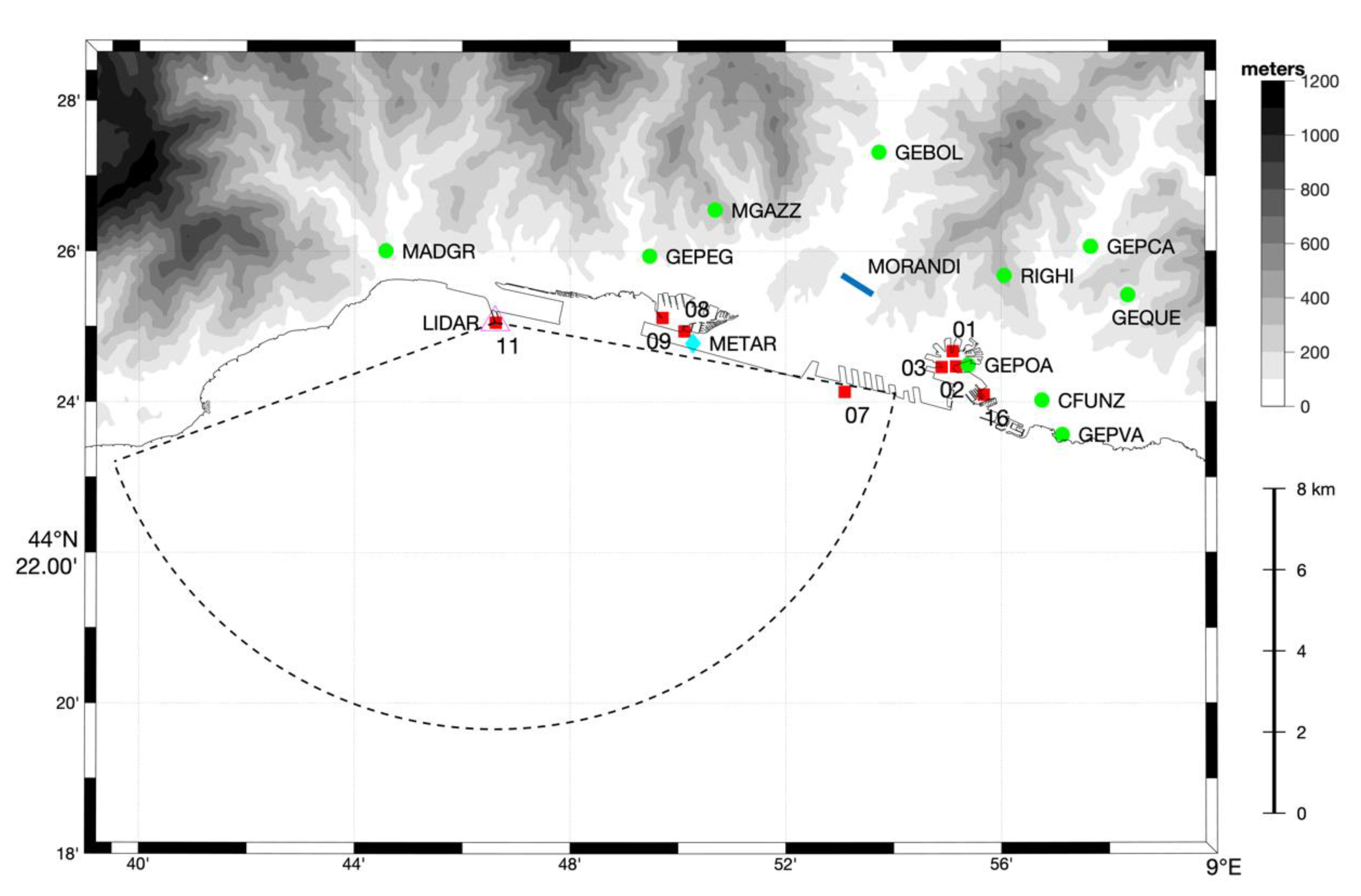
2.1. Meteorological Data

Different data sources were used to describe this event from the synoptic to the local scale. The synoptic meteorological conditions were analyzed utilizing the Global Forecast System (GFS) analyses of the National Centers for Environmental Prediction (NCEP) that are available on a 0.5° × 0.5° grid every 6 h. The development of the thunderstorm that approached Genoa from the southwest was monitored using the meteorological radar of the Liguria Region, which is operated by the Italian Meteo-radar Network. The radar range is approximately 100 km. The lightning strikes were recorded through the Blitzortung network (http://www.blitzortung.org/), as well as the LAMPINET (Lightning Network of the Italian Air Force Meteorological Service) system [19,20,21]. The local weather conditions were monitored using the meteorological stations of the Meteo-Hydrological Observatory of Liguria Region, operated by the Regional Agency for Environmental Protection (ARPAL), and the weather METAR station of the Genoa Airport. Lastly, the gust front evolution in time and space was analyzed employing the anemometric stations available in the Port of Genoa (managed by the Port Authority, Genoa, Italy) and the lidar scanner (property of the University of Genoa, Genoa, Italy). The lidar scanner was also used to partially reconstruct a gust front that occurred in the precipitation zone of the thunderstorm cloud.

Table 1. Meteorological stations managed by the Regional Agency for Environmental Protection of Liguria Region available in the coastal area affected by the thunderstorm on 14 August 2018.

Station ID	Coordinates (Lon ° E, Lat ° N, Altitude m ASL)	Parameters 1
GEBOL	(8.89561, 44.45530, 47)	T, PR
RIGHI	(8.93433, 44.42797, 360)	T, PR, W
CFUNZ	(8.94591, 44.40035, 30)	P, T, R, PR, RAD
GEPCA	(8.96109, 44.43439, 30)	PR
GEPEG	(8.82460, 44.43227, 69)	T, PR
GEQUE	(8.97260, 44.42367, 200)	T, RH, PR
MADGR	(8.74299, 44.43344, 104)	T, RH, PR
MGAZZ	(8.84485, 44.44247, 310)	T, PR
GEPOA	(8.92317, 44.40816, 25)	W
GEPVA	(8.95222, 44.39278, 10)	W

¹ P = pressure (hPa), T = temperature (°C), RH = relative humidity (%), PR = cumulated precipitation, RAD = mean solar radiation (W/m²), W = wind speed (m/s) and direction (deg).

lists the available meteorological stations in the area that was affected by the investigated thunderstorm. Except for the GEPOA and GEPVA stations (see Table 1 and Figure 1), all other weather stations measured precipitation (PR), but only three of these stations measured wind speed and direction (W). All available measurements are either averaged or cumulated over the 1 h period around the collapse.

Anemometric stations available within the port area are shown in

Table 2. Specification of the anemometric stations managed by the Port Authority of Genoa.

Station ID	Coordinates (Lon ° E, Lat ° N, Altitude m ASL)	Data Coverage 14 August 2018	Data Coverage 09:00–10:00 UTC
01	(8.91838, 44.41119, 16)	66.6	78.8
02	(8.91939, 44.40780, 17)	64.9	81.6
03	(8.91501, 44.40771, 15)	72.4	79.8
07	(8.88499, 44.40220, 15)	84.4	85.7
08	(8.83541, 44.41562, 16)	66.5	90.8
09	(8.82859, 44.41862, 15)	65.9	87.9
11	(8.77698, 44.41754, 25)	62.7	88.0
16	(8.92797, 44.40157, 18)	72.4	78.0

. Unfortunately, wind speed measurements were available with a resolution of 1 m s⁻¹ only, whereas wind direction was available with a 1° resolution. The anemometers’ sampling rate of about 4 s is high enough to allow the evaluation of gust front movement in space and its evolution in time. However, the higher sampling frequency would be needed to report the actual maximum wind speed and turbulence intensity characteristics during the collapse. Data coverage around the collapse time shows the high recovery percentage of valid velocity readings in a period of 1 h centered on the bridge collapse time.

The employed lidar that has been continuously in operation since April 2018 is a 3D scanning WindCube 400S lidar, developed by Leosphere (Orsay, France). Lidar’s PPI (Plan Position Indicator) mode of operation scans the azimuthal range of 100–250° and up to a maximum distance of 14 km in the radial direction. The scanning elevations are between 2.5° and 10° from the horizontal with a 2.5° increment. Each PPI scan requires approximately 50 s to complete. The position of the lidar (and its scanning area) is shown in Figure 1 (magenta triangle) together with the location of anemometer 11 (red square) that is located next to the lidar. The lidar was acquired in the context of the European Project THUNDERR [22] (Detection, Simulation, Modeling and Loading of Thunderstorm Outflows to Design Wind-Safer and Cost-Efficient Structures) with the purpose of thunderstorm monitoring and detection. The instrument has been used to measure the fine structure of gust fronts and downbursts associated with thunderstorm activity. This lidar measures the radial component (i.e., Doppler velocity) of the 3D wind speed in the range ±30 m s⁻¹, and with a gate resolution of 150 m.

Figure 1 shows the position of all meteorological and anemometric stations included in Table 1 and Table 2, as well as the METAR station and the lidar scanner location. The lidar scanner is side by side with anemometer 11, thus the two symbols overlapping each other. The position of Morandi Bridge is also shown in blue. The bridge was in a suburban and industrial area along the Valley of Polcevera, which stretches for approximately 10 km in the south-north direction. The riversides are reaching 600 m ASL (above sea level) in the northernmost part of the valley and around 200 m ASL close to the bridge. Anemometer 07—the closest anemometer to the bridge—was 2.7 km southward from the center of the bridge. The weather station GEBOL was 3.2 km northward from the bridge.

2.2. WRF Model Setup

The Weather Research and Forecasting (WRF) model results are used here to investigate the possibility of predicting this kind of events with numerical weather prediction (NWP) models in operational configuration.

The WRF model [23] is a compressible non-hydrostatic model with mass-based terrain-following coordinates developed at the National Center for Atmospheric Research (NCAR) in collaboration with several institutes and universities for operational weather forecasting and atmospheric science research. This work adopted the WRF version 3.8.1 (Advanced Research WRF dynamic core) and the data assimilation package (WRFDA) version 3.9.1. The two different domain configurations used in the current study are both operationally used since 2018 at the CIMA (Centro Internazionale in Monitoraggio Ambientale) Research Foundation on behalf of ARPAL (Liguria Region Environment Protection Agency).

The first configuration is without data assimilation and uses three nested domains with the horizontal resolutions of 13.5 (250 × 250 grid points), 4.5 (451 × 450) and 1.5 km (943 × 883) and 50 vertical levels (Figure 2a; top of the domains at 50 hPa). This setup was used to produce two different forecasts: (1) the first using the initial and lateral boundary conditions from the NCEP-GFS (National Centers for Environmental Prediction—Global Forecast System) with the horizontal resolution of 0.25° × 0.25° and a 3-h time resolution (hereafter WRF-GFS); and (2) the second using ECMWF-IFS (European Center for Medium-Range Weather Forecasts—Integrated Forecasting System) forcing with the horizontal resolution of 0.125° × 0.125° and a 3-h time resolution (hereafter WRF-IFS).

The second domain setup is composed out of three nested domains with the horizontal resolution of 22.5 (76 × 73 grid points), 7.5 (172 × 163), and 2.5 km (346 × 316) and 50 vertical levels (Figure 2b). The two numerical simulations performed using this setup, as in the previous case, relied on the NCEP-GFS and ECMWF-IFS initial and boundary conditions, but with the additional implementation of a Three-Dimensional Variational (3DVAR) data assimilation. In this study, the 3DVAR method is employed with a 3-h cycling update technique. The basic goal of this technique is to provide an optimal estimate of the true state of the atmosphere through the minimization of a proper cost function [24]. To distinguish them from the first setup, these two simulations are hereafter referred to as the WRF-GFS-DA and WRF-IFS-DA, respectively.

The WRF-GFS-DA and WRF-IFS-DA runs include a first 3DVAR assimilation at 00:00 UTC. The model then produces a 3-h forecast followed by the second assimilation cycle at 03:00 UTC and later the third assimilation cycle at 06:00 UTC; afterwards, the model generated a 24-h forecast. The 3DVAR method was employed here consistently with the WRF operational configuration to assimilate radar reflectivity into the WRF model. The data assimilation was performed following the procedure in Lagasio et al. [25] by using the modified direct operator described in Equation (11) in Reference [25]. All simulations in this study were initialized at 00:00 UTC on 14 August 2018.

All simulations were performed with the same set of physical parameterizations that have been successfully tested in several studies of similar events [25,26,27]. The surface layer was modeled using the Mesoscale Model 5 (MM5) scheme that uses the stability functions from Reference [28,29,30] to compute surface exchange coefficients for heat, moisture, and momentum. Convective velocity calculations from Reference [31] were used to enhance surface fluxes of heat and moisture. The Rapid Update Cycle (RUC) scheme with 6 soil levels (0, 5, 20, 40, 160, 300 cm) was utilized for the parameterization of land surface processes. The soil model solves the heat diffusion and Richards moisture transfer equations with the layered discretization [32,33]. The planetary boundary layer (PBL) dynamics was parameterized with the diagnostic non-local Yonsei University PBL scheme [34], which accounts for counter gradient terms to represent fluxes due to non-local gradients and has explicit treatment of the entrainment layer at the PBL top. The entrainment is made proportional to the surface buoyancy flux in line with results from studies using large eddy simulation models [35]. This study used the WRF-single-moment 6 (WSM6) microphysics scheme with six classes that include the prediction of graupel and other microphysics processes [36]. Finally, the radiative processes were parameterized using the longwave and shortwave Rapid Radiative Transfer Model for General Circulation Models (RRTMG) schemes [37]. The results of Parodi et al. [11] are used to derive the deterministic model setup used here. The model setup chosen is the best-performing one among the ensemble previously studied in Reference [11] for similar conditions over the same area.

3. Results and Discussion: Observations

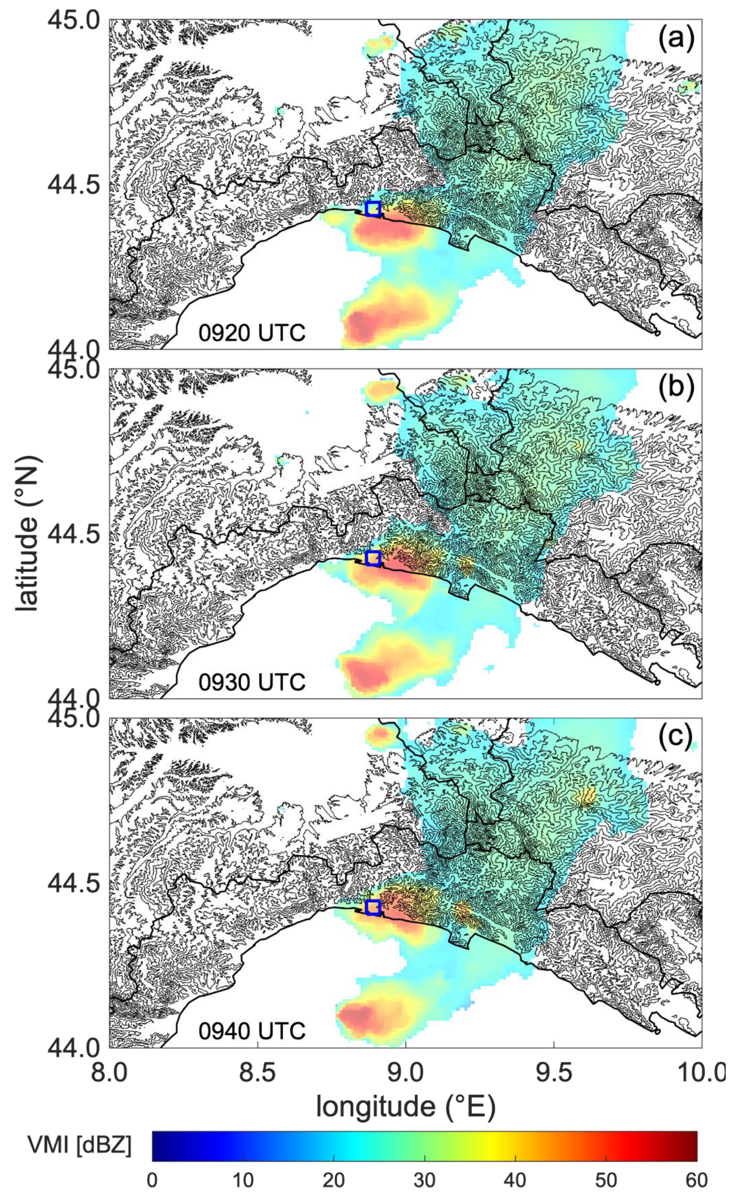
3.1. Weather Conditions at Large Scales

Between 16 and 19 August 2018, two low-pressure systems, Querida and Roswitha (following the naming convention used by the Institute of Meteorology of the Freie Universität Berlin, Berlin, Germany), initially located at the latitudes approximately between 55–65° N, traveled eastward following the main sub-arctic zonal flow along the storm track through the Atlantic Ocean to Northern Europe. On 18 August, at 00:00 UTC, these two depressions were situated over the northwestern Scandinavia (Querida I and II) and to the east of Iceland (Roswitha) (Figure 3a). Along with these depressions, a trough that extended in the meridional direction down to the Northern Mediterranean caused instability along its path as it moved from the Bay of Biscay to the north of Italy. On the morning of 18 August, a secondary pressure minimum developed over the Gulf of Lion and moved eastward over the Ligurian Sea bringing an intensive thunderstorm activity. While this severe weather was particularly pronounced in the coastal areas of northwestern and central Italy, it rapidly disappeared in the afternoon. The tropopause height contour at 11,000 m (Figure 3b; green contour) indicates that the position of the tropopause cutoff was associated with the secondary cyclogenesis that occurred in the lee of the Alps. The similar triggering mechanism of severe weather in the Gulf of Genoa was also reported in Reference [2].

Slow time evolution of deep convective clouds above the Gulf of Genoa can be observed between 09:15 and 10:00 UTC (Figure 4) from satellite images. Although the four instances of cloud top heights shown in Figure 4 look similar, the noticeable feature in these images is the convection that started to develop between two previously disjoint cloud clusters. We observe that the clouds above the Genoa region at 09:15 UTC were not connected to the cloud system that developed south from Genoa and west from Corsica. Over the next 45 min, the two regions merged to form a long convective line that stretched in the south-north direction. Around 09:45 UTC, the tops of convective clouds above Genoa were still at 12,000 m, thereby indicating the strong and well-developed convection. These deep cumuliform clouds were responsible for the observed gust front that was detected before the bridge collapse and are discussed later in Section 3.3.

The radar images in Figure 5 show the existence of two dominant precipitation cells characterized by a strong radar reflectivity that exceeded 55 dBZ. The north cell was initially situated southwest of Genoa (Figure 5a), but, in the next 20 min it moved in the northeast direction, and finally between 09:30 and 09:40 UTC, it was situated above the city. The south cell, on the other hand, stayed stationary throughout this process. One of the interesting features of the northern precipitation cell is its deformation that is manifested as deeper propagation of the central precipitation zone in the north direction. Between 09:20 and 09:40 UTC, the isoecho of 40 dBZ propagated approximately 6800 m inland from the coastline, where it was at 09:20 UTC. Therefore, the northward propagation velocity of precipitation cell that traversed Genoa around the bridge collapse time was about 5.7 m s⁻¹. The northward movement of the precipitation cell is likely to be influenced by the orographic channeling that can be inferred from Figure 5. While the bottom of the two valleys is below 100 m ASL, the mountains on both sides of the valleys that run across Genoa rise to almost 10:00 m ASL. The location of Morandi Bridge in the west valley of Genoa is shown in Figure 5, with respect to the precipitation cell. The influence of orography and river valley on thunderstorm propagation was investigated in Reference [38]. The authors concluded that thunderstorms influenced by orographic effects are more compact in comparison to thunderstorms over flat terrain. This difference is caused by the smaller and unidirectional (only along the direction of the valley) supply of low-level moisture in the orographic case. However, the numerical study of Ćurić et al. [38] was carried out for a different geographic region (the Balkan Peninsula), and more research is needed on the influence of orography on gust fronts and thunderstorm propagation, particularly in coastal regions.

The 5-min Surface Rainfall Intensity (SRI) estimates from the national mosaic of the Italian Meteo-Radar Network is here used to evaluate the storm cell motion towards the coast in the period between 09:00 and 10:00 UTC. The application of the region growth algorithm to the binary image rain/no rain [39] shows that the cell was isolated from the rest of the precipitation field observed at larger scales. The center of mass of the precipitating cell was identified, and the cell centroid displacement between subsequent images was used to evaluate speed and direction of the cell.

The results in Figure 6 demonstrate that the precipitation cell was moving north-eastward until 09:25 UTC, when the cell reached the coast. Once landed, the cell intensity decayed, its shape from approximately elliptical changed to an arrowhead-like shape pointing northward as it wedged along the Polcevera Valley. At the same time, the translation speed reduced to almost 2 m s⁻¹, and the propagation direction backed almost 90° from 09:25 to 09:45 UTC. The translational speed of the cell approaching the coast was around 4 m s⁻¹, with a highest speed being exceeding 6 m s⁻¹ between 09:15 and 09:25 UTC.

This pronounced convective activity above Genoa and south from the city was also detected by the Blitzortung network for lightning strikes detection (Figure 7a). We observe that the lightning strikes were organized along the south-north line that stretched from the north part of Corsica to the north of Genoa. These results show that the lighting was predominantly concentrated over the convective line situated above the sea, and the number of lightning strikes above Genoa was less significant.

The position of lightning strikes measured through LAMPINET has an accuracy of 500 m (Figure 7b,c). In the bridge collapse hour, lightning strikes were mostly recorded over the sea (Figure 7b) and later over the coast and east part of Genoa (Figure 7c). The largest number of strikes occurred between 09:35 and 09:40 UTC at 4–5 km from the bridge, in the area around the Old Port of Genoa. The spatial extent of the cumuliform clouds in Figure 4 was predominantly in the west-east direction, which is not necessarily the dominant direction of the zone characterized by the highest frequency of lightning strikes around Genoa (Figure 7b,c). We also report that the lightning strikes were not observed by LAMPINET in the vicinity of the Morandi Bridge (thick black line).

Due to the high lightning activity, the initial speculation that appeared in newspapers was that lighting could have struck the stays or rain could have destabilized the base, thereby causing a landslide. While these hypotheses were abandoned soon after, the possibility that strong winds could have played a role in the bridge collapse was considered an unlikely option by experts at the beginning of their investigations. This study also demonstrated that the possibility a lightning strike triggered the bridge collapse is minimal. Despite this lack of wind investigation, the weather is officially ruled out as a contributing factor for the bridge collapse, at least at the time of writing this study. Nevertheless, the current meteorological analysis of weather conditions that occurred in Genoa at the time of the bridge collapse is a relevant study to support the weather hypothesis in bridge collapse or possibly reconsider the role of weather in this disaster.

3.2. Local Observations

Even if quantitative measurements of weather conditions in the immediate bridge vicinity are not available, it is evident based only on the video available very close to the accident (released by the Italian Finance Guard on 1 July 2019 and taken from a security camera placed about 150 m to the west of the bridge), as well as many eyewitnesses, that severe weather conditions were present at the bridge around the time of the collapse. Figure 8 shows two frames extracted from the video at the time of collapse (Figure 8a) and few seconds immediately after the bridge had fallen (Figure 8b). The arrow in Figure 8a shows the lighting that occurred to the east-southeast of the bridge during the collapse, while Figure 8b depicts the cloud of dust and debris at the ground that was caused by the collapsed bridge (see Arrow 1). The finest particles in the dust cloud were suspended in the air and advected to the left of the photo by the wind that was blowing from south to north. Arrow 2 in Figure 8b shows the strong inclination of a tree to the left, therefore confirming that a strong wind was likely blowing at the time of the collapse. The full event recorded in the video, which is considered relevant to this study, is available at: http://www.gdf.gov.it/stampa/ultime-notizie/anno-2019/luglio/video-del-crollo-del-viadotto-polcevera-ponte-morandi-del-14-agosto-2018#null.

The standard METAR meteorological measurements from the Air Force weather station of the Genoa Airport are shown in Figure 9. The temporal resolution of data is not consistent throughout the records, but, on average, the wind velocity and air temperature data are available every 20–30 min. The temporal resolution of pressure data is at every approximately 2.5 h. Figure 9a shows that the wind direction at the time of bridge collapse abruptly changed for almost full circle (i.e., from 350° to approximately 10° from 08:50 to 10:20 UTC) in the counterclockwise direction. At the exact time of the bridge collapse, the wind was blowing from 140° (southeast). Around the same period, the mean wind speed increased from approximately 2 m s⁻¹ to 7.7 m s⁻¹ at the time of collapse (Figure 9a). Afterwards, the wind speed declined to about 4.5 m s⁻¹ at 1000 UTC. Bearing in mind that the values are 10 min averages, the mean velocity of ~8 m s⁻¹ demonstrates that the event was characterized with relatively low wind speeds. For example, this value corresponds to a wind speed with return periods lower than two years in Liguria [40]. This is further confirmed by observing the recorded wind gust of 16 m s⁻¹ at 09:50 UTC (14 min after the collapse), which is the overall maximum value that was measured from 09:40 to 09:50 UTC. Note that, in the time interval between 09:40 and 09:50 UTC, the mean (maximum) wind speeds measured at the ARPAL weather stations GEPOA and GEPVA (see Figure 2) were 7.9 (16.1) m s⁻¹ and 5.9 (15.5) m s⁻¹, respectively. The prevailing wind directions were from south and west-southwest, respectively.

An important validation that the event was a thunderstorm downburst comes from the analysis of wind velocity records in conjunction with air temperature and pressure data (Figure 9b,c). In our case, the air temperature is a more useful quantity due to the higher temporal resolution of these data. Figure 9b shows that a decrease in temperature occurred simultaneously with the increase of surface wind speed and abrupt shifts in wind direction (Figure 9a). The decrease of temperature at 08:50 UTC coincides precisely with both the increase of wind speed and abrupt change of wind direction. In the next hour (until 09:50 UTC), the temperature dropped for 4 °C. The subsequent increase of surface air pressure (Figure 6c) also follows the kinematics and dynamics theory of gust fronts, but the low temporal resolution of data prevents a more comprehensive analysis.

The accumulated surface precipitation in the collapse hour increased in the eastward direction (Figure 10). While precipitation was not observed in the western parts of the port, the east side received 33.8 mm h⁻¹ of rain between 09:00 and 10:00 UTC. The weather station situated in the same valley as Morandi Bridge (GEBOL; Figure 10) and approximately 3.2 km north of the bridge, received 12 mm h⁻¹ of rain. Therefore, the zone of the strongest precipitation coincided with the area characterized by the highest activity of lightning strikes (Figure 8). We also observe that the heavy rain (i.e., >10 mm h⁻¹) was localized at the GEBOL, RIGHI, and CFUNZ stations (Figure 10), thereby indicating that Morandi Bridge probably received around 10 mm h⁻¹ of rain in the collapse hour. However, since the weather stations cover approximately two times longer area in the zonal direction than in the meridional direction, the observation that the variability of precipitation in the west-east direction is larger than in the south-north direction might be skewed. No hail nor other ice particles were observed in this period at any weather station in the Genoa region.

Further, we discuss the high-frequency velocity records from the anemometers located along the Port of Genoa. The position of these stations is reported in Table 2 and is shown in Figure 2. In the hour centered around the collapse time (09:36 UTC), for the majority of stations, the wind direction was continuously changing in the counterclockwise direction starting around the north direction at the beginning of the hour (about 09:00 UTC) and returning to the north direction at the end of the hour (about 10:00 UTC) (Figure 11). Notice that the same trend was also observed in Figure 9. Although the counterclockwise change of wind direction is observed at all eight anemometers, the shift is less pronounced at the anemometers 08, 09, and 11. These three anemometers are in the west part of the port area and approximately 5–10 km away from the other five stations. The wind direction at the time of the bridge collapse was approximately 180° at the anemometer station 07. At the same time, in the east stations (03, 01, 02, 16), the wind was blowing from the third quadrant (between 180° and 270°), whereas the west stations (08, 09, 11) recorded the wind direction from the second quadrant (between 90° and 180°). This spatial distribution of wind directions resembles the cloud-scale (~10 km) radial outflow produced by the gust front, which was spreading from underneath the cloud base.

Similarly, the wind speed records also exhibit noticeable differences between the west and east parts of the port (Figure 11). The differences between the peak wind speed close the bridge collapse time and the wind speed at the beginning of that hour are higher at the anemometer stations located in the east part of the port (Figure 11e–h). The velocity records in the west and central parts of the port (Figure 11a–d), on the other hand, show pronounced nonstationary signature before the velocity peak that occurred around the collapse time. Figure 11 shows clearly that the maximum wind speed—which occurred before 09:36 UTC for stations 07, 08, 09, 11, and after the collapse time for stations 01, 02, 03, 16—had a slight time shift from the westernmost to the easternmost anemometer. This can be interpreted as the signature of the gust front passage that follows the cloud translation from south-west to north-east over approximately 15 km of the coast. This result is in accordance with the estimated movement of precipitation zone in Figure 7 and Figure 8. All anemometer measurements (Figure 9 and Figure 11) show that the near-surface wind velocities around the collapse time were approximately two times smaller than a velocity in the weakest tornado (EF0-rated; 29 m s⁻¹).

Overall, these results demonstrate that the thunderstorm produced a gust front that originated over the sea and approached the anemometers, as well as the bridge, from the prevailingly south direction. This is shown in Figure 12, which is a representation of the wind velocity vectors (1 min averaged) obtained from the measurements of the 8 anemometers in the Port of Genoa: Figure 12a depicts the situation prior to the thunderstorm occurrence, at 08:50 UTC when the wind was blowing from the mountains; Figure 12b shows the gust front that, at 09:25 UTC, had reached the western stations; afterwards, the outflow intensifies and affects all stations (Figure 12c), which, at 09:35 UTC, showed a radial outflow-like diverging pattern (notice the southerly flow at station 07 that possibly produced a flow channeling in the Polcevera Valley towards the bridge location, indicated by the blue line); finally, at 09:40, the outflow center had moved to the east of the stations, as all the wind vectors pointed westward.

Recently, Burlando et al. [15] demonstrated that the majority of thunderstorm downbursts in this region are generated over the sea and then advance towards the shore. A similar trend in terms of downburst formation and movement was also reported by Burlando et al. [2] for a downburst event in the Port of Livorno, Italy, on 1 October 2012. As already discussed in relation to the METAR measurements presented in Figure 9, the gust front was relatively low-intensity as the maximum velocity recorded at all anemometer stations was in the order of 15 m s⁻¹.

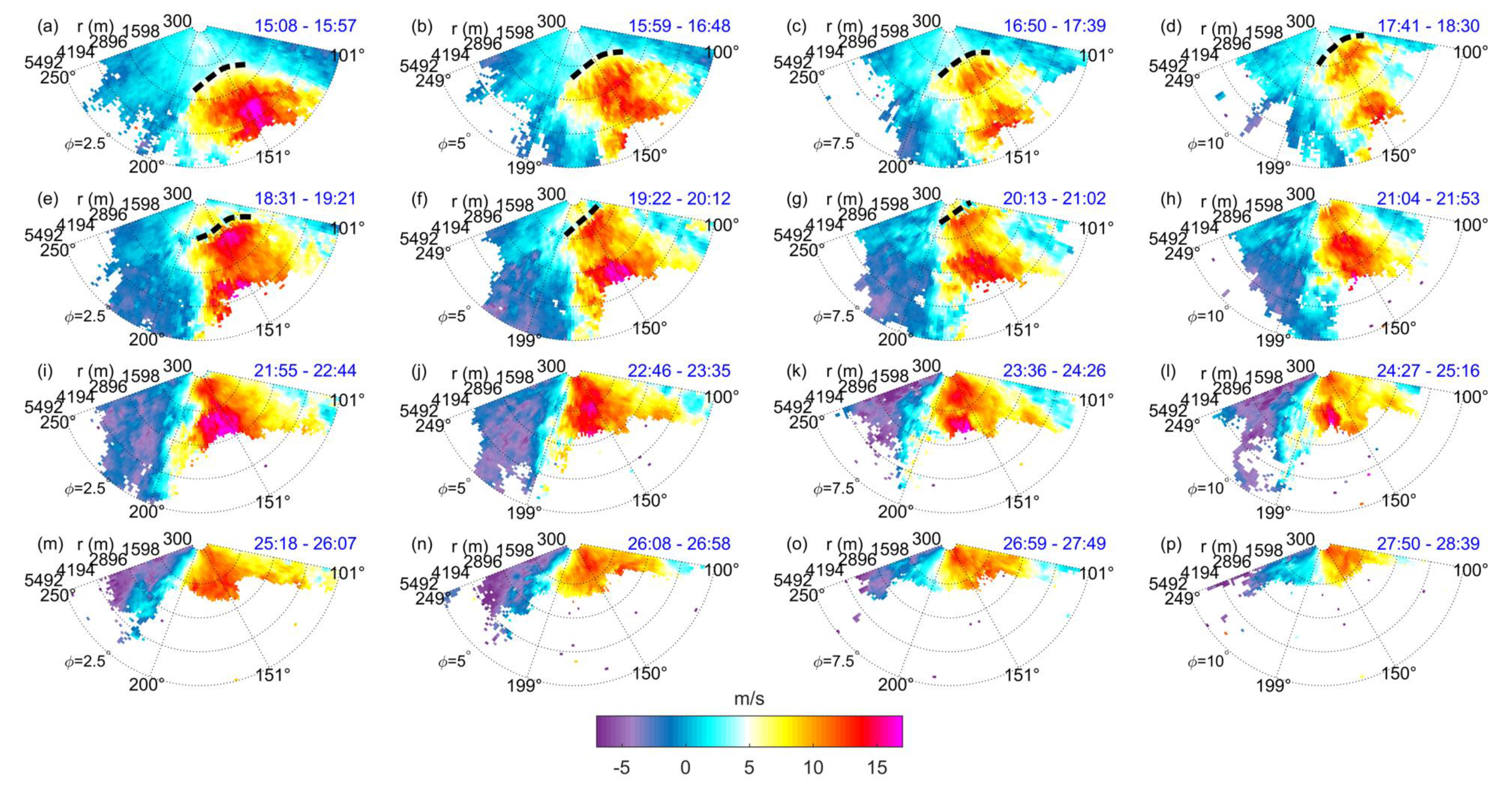
3.3. Lidar Gust Front Detection and Analysis

Approximately 15 min prior to the bridge collapse (i.e., between 09:20 and 09:35 UTC), the thunderstorm gust front was also captured by the Doppler lidar installed in the Port of Genoa (Figure 13). Note that the timing of the gust front in Figure 13 is coherent with the maximum wind speeds recorded by anemometer 11 (Figure 11). The lidar scanned four different elevation angles ($\phi$) between 2.5° and 10° above the horizontal plane with a 2.5° increment. These results are particularly interesting because Figure 13 is among the few sets of published lidar velocity measurements of a thunderstorm gust front [41]. Unfortunately, the heavy rain that occurred behind the gust front affected the lidar measurements by reducing the range of data acquisition from about 5 km at 09:15 UTC to 1–2 km at 09:30 UTC.

This thunderstorm gust front was characterized with the velocities exceeding 20 m s⁻¹ (Figure 13). The highest positive velocities (i.e., towards lidar) are observed at the lowest $\phi$ and between 09:15 and 09:23 UTC. Besides, Figure 13 shows the propagation of the region characterized by the maximum velocity towards lidar (observed for all $\phi$ angles). The direction of the maximum velocity is from 150° until approximately 09:23 UTC (Figure 13i), and then it starts shifting in the clockwise direction eventually reaching ~170° (Figure 13k). The width of this region is at least 3.5 km. However, the width of this region could have been larger but not detectable by the lidar due to the limited azimuthal scans. The azimuthal orientation ($\theta$) of the zone with the maximum velocity seems to be independent of height, which indicates that the advancing gust front is not (significantly) inclined in the $\phi -\theta$ plane. However, it is particularly important to note that, with increasing $\phi$, this region of the maximum velocity is inclined towards lidar. For example, when benchmarked against Figure 13a ($\phi =2.5°$), this region is closer to lidar in Figure 13d ($\phi =10°$) than it is in Figure 13e ($\phi =2.5°$), although the velocity slice in Figure 13e is later than the one in Figure 13d. The continuous advancements of this front between the elevations of $\phi =2.5°$ and $\phi =10°$ are nicely observed in Figure 13b,c for $\phi =5°$ and $\phi =7.5°$, respectively. Moreover, the same trend is found in the next set of four velocity slices, shown in Figure 13e–h. That is, at $\phi =2.5°$ (Figure 13e), the front is approximately 2000 m away from lidar, while, at $\phi =10°$ (Figure 13h), the front is already above lidar (or within 300 m away from the instrument). The distances between these two are found at the other two intermediate elevations.

This displacement of the region of the maximum velocity with height is a characteristic of the radially advancing gust front of cold air in front of the thunderstorm cloud [42,43,44,45,46]. Further, Figure 13 enables the estimates of the displacement velocity of the gust front towards the lidar. Figure 14 shows the height ASL of the gust front (black dashed line in panels a–g) at different radial distances from the instrument along $\theta =151°$. For the height corresponding to 120 m ASL (i.e., 115 m above lidar level plus 5 m ASL, which is the height of the lidar ASL), we estimate the displacement velocity ($V_d$) of the gust front to be $V_{d1}=6.3{\mathrm{m}\mathrm{s}}^{-1}$ towards the instrument. A similar displacement velocity, $V_{d2}=6.9{\mathrm{m}\mathrm{s}}^{-1}$, is obtained at 70 m ASL (i.e., 65 m above lidar). Thus, an average displacement velocity component towards the lidar is evaluated to be $V_d=6.6{\mathrm{m}\mathrm{s}}^{-1}$. Note that this velocity is about 1–2 m s⁻¹ larger than the estimated velocity of the north-eastward propagation of the precipitation cell in the radar images (Figure 6). The displacement velocities calculated above are very similar to the one estimated by Mueller and Carbone [44] by tracking radar reflectivity and Doppler velocity of a gust front associated with a thunderstorm outflow measured in Denver, Colorado, USA, in 1984. They obtained a value of 6.9 m s⁻¹.

When combined with the meteorological measurements from the Genoa Airport weather station (Figure 9) and precipitation measurements in the area (Figure 10), this displacement velocity can further be used to estimate the mean height of the cold inflow [42]. We used the Genoa Airport weather station in this analysis due to its proximity to the coastline and effectively the same elevation as the lidar. The other weather stations listed in Table 1 are located at higher elevations; therefore, the gust front structure and atmospheric conditions differ from those observed at the sea level. First, we estimate the mean air densities of the ambient and gust front air masses. The air density ($\rho$) is calculated using the equation of state for wet air:

$$\rho =\frac{p_d}{R_{d}T}+\frac{e}{R_{w}T} ,$$

(1)

where $p_d$ and $e$ are the pressure of dry air and water vapor (in Pa), respectively, $T$ is the air temperature (in K), $R_d=287.058$ J kg⁻¹ K⁻¹ is the gas constant of dry air, and $R_w=461.495{\mathrm{J}\mathrm{kg}}^{-1}{\mathrm{K}}^{-1}$ is the gas constant of water vapor. Since the relative humidity during the investigated period was ~100%, $e$ is equal to the saturation water vapor pressure ($e_s$) because the dew point is equal to air temperature. The relationship between $e_s$ and air temperature can be expressed through the August-Roche-Magnus formula as [47]:

$$e_s=e_{s0}\exp \left(\frac{A_{1}t}{A_2+t}\right),$$

(2)

where $e_{s0}=610.94\mathrm{Pa}$, $A_1=7.625$, $A_2=243.04℃$ [48], and $t$ is the air temperature (in °C). Further, the pressure of dry air is calculated using Dalton’s law of partial pressures as:

$$p_d=p-e=p-e_s,$$

(3)

because of $e=e_s$ (i.e., the relative humidity of ~100%). Here, $p$ is the measured (total) atmospheric pressure of wet air (in Pa). Plugging in the temperature drop of 4 K (from 296.15 K, i.e. 23.2 °C, to 292.15 K, i.e. 19.0 °C) and the pressure rise of ~130 Pa (~1.3 mb) into the above Equations results in the air densities of cold (gust front) and ambient air being ~1.2024 kg m⁻³ and ~1.1833 kg m⁻³, respectively.

Then, we further use the equation for displacement velocity ($V_d$) of gravity currents (e.g., Reference [42,49,50,51]) to estimate the mean depth of the cold inflow:

$$V_d=k\sqrt{gd\frac{{\rho }_2-{\rho }_1}{{\rho }_1}},$$

(4)

where ${\rho }_1$ and ${\rho }_2$ are the densities of warm (ambient) and cold (gust front) air masses (in kg m⁻³), $g=9.8053{\mathrm{m}\mathrm{s}}^{-1}$ is the gravitational acceleration at 44° N and sea level, and $k=0.77$ [45,52] is the constant that represents the ratio of internal to gravitational forces [42]. Lastly, $d$ is the unknown mean depth of the cold inflow (in m) that will be obtained. The value of $k$ is uncertain and other numbers were proposed, too [50,51]. Solving Equation (4) for $d$ yields the value of $d=464\mathrm{m}$. A value of 478 m is obtained if the air is assumed to be dry. For instance, Charba [42] used Equation (4) to estimate the displacement velocity of 22.7 m s⁻¹, but the measured value of $d$ in his study was 1350 m. The surface air pressure rise (~677 Pa) and temperature drop (~5 °C) in his work were larger than in our case. In addition, our velocity estimate is only the component towards the lidar of the overall propagation velocity. However, smaller values of $V_d$ and $d$ than in Charba [42] were also reported by Goff [53] and Mueller and Carbone [44].

Besides the value of $k$, another uncertainty associated with the above analysis is related to the usage of surface air densities in Equation (4), instead of the mean air density along the height of the gust front inflow. Unfortunately, temperature and pressure profiles at this location are not available for this event. Since the air density difference ${\rho }_2-{\rho }_1$ is usually constant with height [42] and ${\rho }_1\left(z>0\right)<{\rho }_1\left(z=0\right)$, the obtained value likely represents the upper limit of $d$. The higher wind speeds associated with the gust front passage (Figure 11 and Figure 13) in comparison to displacement velocity of the gust front (Figure 14) are expected and reported elsewhere, too [42]. According to Goff [53], the slowly moving gust fronts, such as the one reported in this paper, are usually associated either with intensifying storms and accelerating outflow or with dissipating storms and decelerating outflows.

The gust front leading edge was inclined in the direction of propagation (i.e., towards lidar) due to the increase of wind speed with height in the outflow (dashed line in Figure 14). The angle of inclination depends on density differences between ambient and gust front air masses, and wind speed, among other factors. In the analyzed case, the inclination angle is −10.1° from the horizontal plane, with the minus sign indicating the negative inclination concerning the measurement location. That is, the gust front surge line increases for 177 m km⁻¹, which is very similar to the result of Charba [42], who obtained the value of 150 m km⁻¹ for a gust front that occurred in central Oklahoma, USA. This comparative analysis indicates that the surface roughness might not be the dominant factor that governs the slope of the gust front leading edge (i.e., gust front surge line) because similar values are obtained for two profoundly different surface roughness characteristics. However, this subject deserves more research and a larger sample of data to confirm this assumption.

Further partial reconstruction of this event is possible by applying various relationships between the height of cold inflow ($d$) and other features of the gust front. According to several studies that investigated gust fronts at full scale or using physical experiments and numerical simulations (e.g., Reference [42,43,45,53]), the height of the leading edge ($H$; called gust front head) is usually $H\cong 2d$. This relationship enables us to further sketch the likely shape of the gust front that occurred over the sea approximately 15 min before the bridge collapse (Figure 15). The height of the gust front nose (265 m) is estimated from Reference [42], where it was reported this height is approximately $d/1.8$. However, other relationships were proposed in Reference [53], too; hence, there is an uncertainty associated with this estimate. Recall that the height of the gust front nose is not the height of the maximum horizontal wind speed in the outflow. The maximum wind speed in downburst outflows is usually observed in the layer between 80 and 120 m above ground [54]. This is in accordance with the findings in Figure 13, which shows that the highest Doppler velocities are measured at the elevation $\phi =2.5°$. The slope of ~70° of the gust front head outline in the region above the gust front nose is simply adapted from Goff [53], while the gust front head height (928 m) is estimated through the relationship $H\cong 2d$. The region behind the gust front head is characterized by pronounced turbulence due to the Kelvin-Helmholtz instability [55]; therefore, there is no clear outline of the gust front edge in that part (notice that the blue dotted lines are not connected behind the gust front head in Figure 15). In accordance with the gust front and downburst outflow theories [42,44,45,46], Figure 13c–h demonstrate that the gust front was associated with two high-speed regions that were separate with the zone of smaller wind speeds. The above-referenced studies demonstrated that the cold inflow typically comes in periodic surges, which is further schematically depicted in Figure 15.

To conclude the discussion on lidar data, Figure 16 shows the lidar velocities around the collapse time. The gust front that was observed in Figure 13 moved away from the lidar, and only small radial velocities (below 10 m s⁻¹) were measured around the bridge collapse time. A positive (towards lidar) and negative (away from lidar) velocity regions were detected for $\theta <150°$ and $\theta >200°$, respectively, at all four elevation angles. Wind speed was slightly increasing with height. Around the collapse time (09:36 UTC), the core of precipitation cell in Figure 7 had already passed over the lidar; therefore, the negative Doppler velocities for $\theta >200°$ are observed. After 09:40 UTC, Figure 7 shows that the precipitation zone was located east of the lidar, which results in the observed easterly winds at the location of the lidar (Figure 16).

4. Results and Discussion: WRF Numerical Simulations

The WRF numerical simulations results have been firstly analyzed by computing 5-min maximum wind speeds at 10 m above ground and the location of the eight anemometers in the Port of Genoa. The considered period is 06:00–15:00 UTC. The WRF-IFS, WRF-GFS, WRF-GFS-DA, and WRF-IFS-DA predictions have been interpolated at the anemometer locations employing the nearest neighbor interpolation method. The results in Figure 17 show that the WRF-IFS experiment is capable of predicting a maximum wind speed up to 11 m s⁻¹ in the period between 08:00 and 09:00 UTC. The same model predicts even higher maximum wind speed between 12:00 and 13:00 UTC. The WRF-IFS-DA forecasts a maximum wind speed up to about 10 m s⁻¹ in the period between 08:00 and 09:00 UTC, whereas the maximum wind speeds around 13 m s⁻¹ are predicted for the period 11:00–12:00 UTC (Figure 17d). Conversely, the WRF-GFS and WRF-GFS-DA simulations produce significantly lower values of the 5-min maximum wind speeds at all eight locations.

To gain a deeper understanding of this thunderstorm system, the Vertical Maximum Intensity (VMI) maps of radar reflectivity from the four WRF simulations were plotted at the time of the wind speed maxima indicated with dashed vertical lines in Figure 17. The first two peaks in all time-series are assumed to occur roughly at the same time in all WRF configurations, i.e., the velocity peaks at 08:30 and 09:55 UTC (Figure 17). The last velocity peak, which is also the most intense event, occurs at 1240 UTC in the WRF-IFS simulation, at 13:25 UTC in the WRF-GFS, at 13:10 UTC in the WRF-GFS-DA, and at 11:30 UTC in the WRF-IFS-DA. For further comparison between the mode and observations, Figure 18a–c show the VMI measurements at 08:30, 09:55, and 13:25 UTC and their modeled counterparts. The VMI observed at 12:40 and 13:10 UTC are not reported in Figure 18 because reflectivity patterns were analogous to the ones at 13:25 UTC (Figure 18c). In general, one can observe that there is no correspondence between the concurrent reflectivity patterns of numerical simulations and observations. This finding is not surprising because numerical weather prediction models often introduce a time and space shift between forecast and measurements. This bias is usually more pronounced for small-scale phenomena, such as a single-cell thunderstorm. Some deep convective spots with the VMI values above 40 dBZ occur in all the four WRF simulations at 08:30 and 09:55 UTC (Figure 18d,g,j,m,e,h,k,n), but these structures are rather small, organized along narrow stripes from southwest to northeast, and they do not resemble the VMI patterns in Figure 18a,b.

Instead, the observations at 08:30 and 09:55 UTC are more similar to the convection developed by WRF-IFS in the early afternoon at 1325 UTC (Figure 18c) and WRF-IFS-DA at 1130 UTC (Figure 18i). In particular, the near-surface wind speeds in the WRF-IFS-DA simulation reach approximately 20 m s⁻¹ at 10 m above ground level (AGL) between 11:00 and 11:55 UTC in the central-eastern Liguria coastline. This value is close to the maximum velocities observed in anemometric measurements around the collapse time (Figure 11). Furthermore, the model shows the development of a gust front that originates from underneath the thunderstorm cloud. We also notice that the assimilation of the radar data into the GFS seems to initiate a convective motion between 11:00 and 12:00 UTC (Figure 17c), but the velocities do not reach the values observed in the WRF-IFS-DA (Figure 17d). Because the WRF-IFS-DA run provided the most accurate simulations of this thunderstorm event, the focus of the following discussion is mainly on these results.

The thermodynamic conditions from the WRF-IFS-DA run at 11:30 UTC are favorable for the onset of strong single-cell thunderstorms (Figure 19), such as the one observed during the bridge collapse. The skewT-logp diagram has been extracted for the central region of the convective system (Figure 19b; Lon 8.97° E, Lat 44.422° N). The diagram shows the Most Unstable Convective Available Potential Energy (MUCAPE) equal to 1245 J kg⁻¹, which is a value associated with the likely development of thunderstorms in the area. The precipitable water of 49 mm indicates potentially high precipitation rates at the ground. This value is comparable to the accumulated surface precipitation measurements at the CFUNZ station in the east part of Genoa (Figure 10). Further, the high values of the Severe Weather Threat (SWEAT) and Showalter Index (SWI) (391 and −4.6 °C, respectively) indicate a high probability of a severe thunderstorm in the area. Similar conclusions are drawn from the analysis of the Total Totals, K-Index, and Lifted Index (Figure 19). The relatively low values of the wind shear and the Storm-Relative Helicity (SREH) depict the atmospheric conditions that are not favorable for the development of supercell thunderstorms. Finally, it is worth highlighting that the value of the Microburst Windspeed Potential Index (MWPI), which ranges between 0 and 5, is equal to 2.2. This value is indicative of the thermodynamic conditions prone to the occurrence of downbursts [56].

For comparison against WRF simulations, Figure 19a shows the radiosounding measurements at 12:00 UTC taken at Milan Linate Airport, which is approximately 120 km to the north-northeast of Genoa. In Milan, the air very close to the surface is drier with respect to the conditions simulated in WRF. This difference is expected because Genoa is along the sea, and, in August, the sea surface temperature is at the yearly maximum. Moreover, Figure 19b shows a profile extracted in the center of the cloud where the dew-point temperature depression is zero up to 500 hPa. Conversely, in Milan only a very thin cloud layer existed at about 600 hPa, which separated a mid-level layer of drier air between 700 and 800 hPa from a thicker high-level layer of dry air between 550 and 300 hPa. This upper layer is characterized by a nearly pseudoadiabatic lapse rate. A very similar thermodynamic behavior, both from qualitative and quantitative points of view, is observed in the WRF simulation above 500 hPa. The radiosounding profile recorded in Milan depicts the environment prone to wet downburst formation [57,58]. The higher moisture at the low levels due to sea evaporation around Genoa acted to reduce convective inhibition and played a role in increasing the probability of thunderstorm formation.

The WRF-IFS-DA simulation nicely depicts the existence of a strong near-surface outflow that shows diverging pattern of winds in the region south from Genoa (Figure 20). The strongest velocities at 10 m above the ground are observed in south and southwest part of the outflow, and the intensity of the winds increases throughout the hour. The peak wind speeds are around 20 m s^–1. The WRF simulation shows that the highest winds occurred along the south part of the thunderstorm system. This result is somewhat counterintuitive because the thunderstorm was translating towards the north and northeast. Assuming the addition of thunderstorm translation to the radially advancing downburst outflow, the maximum winds would be expected in the northern regions of the outflow. Figure 20 further shows that our measuring network, as well as the bridge (purple cross in Figure 20), were not exposed to the highest velocities in the outflow.

Figure 21a shows an updraft and downdraft (isosurfaces equal to ±1 m s⁻¹) in combination with the maximum 10 m wind speed (shaded colors and vectors). The simulated radar reflectivity in the vertical plan is shown in Figure 21b. Similar to the earlier discussion, the WRF-IFS-DA results show an intense convective activity ahead of the Liguria coastline at 11:30 UTC. The larger scale cyclonic flow patter near the surface (Figure 21a) acts as the main provider of the inflow for the updraft in the forward flank of the thunderstorm. We also observe that the cold downdraft that originated inside the cloud reduces the air temperature at 2 m ASL upon its impingement (Figure 21b). The temperature difference between the cold pool and the ambient air around the thunderstorm is similar to the temperature drop of ~4 K (from 296 K (23.2 °C) to 292 K (19.0 °C)) that was observed at the Genoa airport station around the collapse time (Figure 9). This result also further validates the analytical procedure that was used in the derivation of Figure 15 in Section 3.3.

The WRF-IFS-DA numerical simulation demonstrates that the forecast of radar reflectivity, thermodynamic properties of the atmosphere at larger scales, and wind field at the local scale can potentially be used as a useful tool for determining the meteorological precursors and contributing factors to the development of thunderstorms in this region. The most significant drawback of the current simulations is the delay of the forecasted thunderstorm with respect to the observed event. Similar results in terms of delayed precipitation were also reported in another case study of a severe storm prediction using the WRF model [59]. In addition, in perspective, the current simulations might be used to model gust fronts and downbursts at much finer scales by adopting the proper downscaling techniques or coupling the WRF with other higher resolution and small-scale models (e.g., Reference [60,61,62]). This is further supported by the results of Fiori et al. [26], which concluded the cloud-resolving model resolutions (~200 m) are needed to properly represent the triggering mechanisms of deep convection in this region. However, as mentioned earlier, the goal of this paper was not to test a research setup of the WRF model, but rather the operational configurations that are employed in the daily meteorological practice of Liguria, Italy.

5. Summary and Conclusions

This article analyzed the weather conditions and their dynamics before and during the collapse of the Morandi Bridge on 14 August 2018. This disastrous event that occurred at 09:36 UTC caused 43 casualties. Since the forensic investigation of the collapsed bridge has not pinpointed the exact factors that caused the collapse, the goal of this paper was to provide the contributions in terms of observed and modeled weather conditions around the collapse time. Therefore, the analyses in this study were based on direct meteorological measurements from the weather stations in the area, wind velocity records from eight anemometers installed along the Port of Genoa, remote satellite and radar observations, and the Global Forecast System (GFS) analysis. The local weather station of Genoa Airport recorded the wind gust of 16 m s⁻¹ a few minutes after the collapse time. The time records of air temperature, pressure, and wind velocity from this weather station, as well as the higher frequency velocity measurements from the eight anemometers located along the coastline, showed the well-known signature of transient thunderstorm conditions during the collapse hour. This observation was confirmed using the satellite (i.e., cloud top heights) and radar (i.e., composite radar reflectivity) data. The radar data showed the existence of two cells close to Genoa with a strong radar reflectivity exceeding 55 dBZ. The satellite images, on the other hand, depicted a convective line that stretched in the south-north direction and extended from Corsica to northern Italy (thus, crossing Genoa). The event was also characterized by the high frequency of lightning strikes, but they were not recorded in the close vicinity of Morandi Bridge, but rather a few kilometers east of it.

In addition,, this study presented the rare lidar measurements of downburst outflow in the form of a gust front that advanced ahead of the parent cumulonimbus cloud. Furthermore, we developed and applied a technique for gust front surge reconstruction using lidar measurements and theoretical relationships that analytically link the main parameters of this phenomenon. The displacement velocity of the gust front in the direction of the lidar approximately 20 min before the bridge collapse was estimated to be 6.6 m s⁻¹, and the height of the cold pool behind the gust front head was calculated to be at 464 m. The front was advancing from the sea towards the land and the observed features were measured approximately 10–15 km south from the bridge. Besides, the lidar velocities showed multiple high-velocity regions behind the leading edge of the gust front. These results corroborate well with the estimated translation of the convective precipitation zone from the radar reflectivity observations.

The numerical simulations of this event were carried out using the Weather Research and Forecasting (WRF) model with four different initial and boundary conditions: (1) WRF-IFS (from the European Center for Medium-Range Weather Forecast); (2) WRF-GFS (from the National Centers for Environmental Prediction); (3) WRF-GFS-DA; and (4) WRF-IFS-DA. The WRF-GFS-DA simulation uses the assimilated radar reflectivity data into the GFS analysis, whereas the WRF-IFS-DA run assimilated the radar reflectivity data into the WRF-IFS. While the first three numerical simulations under-estimated the maximum velocity during the bridge collapse hour, the WRF-IFS-DA simulation proved the good matching with the observations. However, it should be noted that all simulations have the tendency to delay the event for several hours (WRF-IFS-DA again provided the smallest delay). The simulated radar reflectivity, near-surface wind field, and thermodynamic indices demonstrated that these products can be used as a valuable tool in the analysis of weather precursors for severe thunderstorms in this region.

In conclusion, this paper demonstrated the existence of a severe thunderstorm in the Genoa region during the collapse of the Morandi Bridge on 14 August 2018. While the strong and transient wind conditions in the form of wet downburst, the associated gust front, and lightning were all present in the minutes before and during the bridge collapse, this study does not firmly conclude that the severe weather was the major triggering factor for the collapse. However, we do acknowledge that the investigated weather conditions might have played some role in the failure of the Morandi Bridge. Future studies on the structural integrity of the bridge under these wind actions are needed.

This article will be complemented in the future with a study that will resolve the entire thunderstorm flow field from the lidar and radar measurements. This activity is ongoing, and the authors are currently facing the difficulty to link together lidar and radar data, as well as to properly reconstruct the three-dimensional wind field inside the cloud from the radial velocity measurements of a single Doppler radar and single lidar. Furthermore, in perspective, the three-dimensional wind field could be assimilated in a cloud model in order to extrapolate the wind flow conditions at the bridge location considering the real thunderstorm evolution and its interaction with topography.

Finally, WRF model is used here to investigate the predictive capability of this thunderstorm by the operational model setup, which assimilates radar reflectivity only. The assimilation of more observations, like radial wind from Doppler radar, could improve the model forecast and will be the subject of future investigations that are currently ongoing.

References

1. NSSL. Thunderstorm Basics. Available online: http://www.nssl.noaa.gov/education/svrwx101/thunderstorms/ (accessed on 27 June 2019).
2. Burlando, M.; Romanić, D.; Solari, G.; Hangan, H.; Zhang, S. Field data analysis and weather scenario of a downburst event in Livorno, Italy, on 1 October 2012. Mon. Weather Rev. 2017, 145, 3507–3527. [Google Scholar] [CrossRef]
3. Radinović, D. Mediterranean Cyclones and Their Influence on the Weather and Climate; WMO: Geneva, Switzerland, 1987. [Google Scholar]
4. Maheras, P.; Flocas, H.A.; Patrikas, I.; Anagnostopoulou, C. A 40 year objective climatology of surface cyclones in the Mediterranean region: Spatial and temporal distribution. Int. J. Clim. 2001, 21, 109–130. [Google Scholar] [CrossRef]
5. Trigo, I.F.; Bigg, G.R.; Davies, T.D. Climatology of Cyclogenesis Mechanisms in the Mediterranean. Mon. Weather Rev. 2002, 130, 549–569. [Google Scholar] [CrossRef]
6. Flocas, H.A.; Simmonds, I.; Kouroutzoglou, J.; Keay, K.; Hatzaki, M.; Bricolas, V.; Asimakopoulos, D. On Cyclonic Tracks over the Eastern Mediterranean. J. Clim. 2010, 23, 5243–5257. [Google Scholar] [CrossRef]
7. Kouroutzoglou, J.; Flocas, H.A.; Keay, K.; Simmonds, I.; Hatzaki, M. Climatological aspects of explosive cyclones in the Mediterranean. Int. J. Clim. 2011, 31, 1785–1802. [Google Scholar] [CrossRef]
8. Drobinski, P.; Ducrocq, V.; Alpert, P.; Anagnostou, E.; Béranger, K.; Borga, M.; Braud, I.; Chanzy, A.; Davolio, S.; Delrieu, G.; et al. HyMeX: A 10-year multidisciplinary program on the Mediterranean water cycle. Bull. Am. Meteor. Soc. 2013, 95, 1063–1082. [Google Scholar] [CrossRef]
9. Romanić, D.; Ćurić, M.; Lompar, M.; Jovičić, I. Contributing factors to Koshava wind characteristics. Int. J. Clim. 2016, 36, 956–973. [Google Scholar] [CrossRef]
10. Zolt, S.D.; Lionello, P.; Nuhu, A.; Tomasin, A. The disastrous storm of 4 November 1966 on Italy. Nat. Hazards Earth Syst. Sci. 2006, 6, 861–879. [Google Scholar] [CrossRef] [Green Version]
11. Parodi, A.; Lagasio, M.; Maugeri, M.; Turato, B.; Gallus, W. Observational and Modelling Study of a Major Downburst Event in Liguria: The 14 October 2016 Case. Atmosphere 2019, 10, 788. [Google Scholar] [CrossRef] [Green Version]
12. Fujita, T.T. Downbursts: Meteorological features and wind field characteristics. J. Wind Eng. Ind. Aerodyn. 1990, 36, 75–86. [Google Scholar] [CrossRef]
13. McDonald, J.R.; Mehta, K.C.; Mani, S. A Recommendation for an Enhanced Fujita Scale (EF-Scale); Wind Science and Engineering Center, Texas Tech University: Lubbock, TX, USA, 2006; p. 111. [Google Scholar]
14. De Gaetano, P.; Repetto, M.P.; Repetto, T.; Solari, G. Separation and classification of extreme wind events from anemometric records. J. Wind Eng. Ind. Aerodyn. 2014, 126, 132–143. [Google Scholar] [CrossRef]
15. Burlando, M.; Zhang, S.; Solari, G. Monitoring, cataloguing, and weather scenarios of thunderstorm outflows in the northern Mediterranean. Nat. Hazards Earth Syst. Sci. 2018, 18, 2309–2330. [Google Scholar] [CrossRef] [Green Version]
16. Solari, G. Emerging issues and new frameworks for wind loading on structures in mixed climates. Wind Struct. 2014, 19, 295–320. [Google Scholar] [CrossRef]
17. Shehata, A.Y.; El Damatty, A.A.; Savory, E. Finite element modeling of transmission line under downburst wind loading. Finite Elem. Anal. Des. 2005, 42, 71–89. [Google Scholar] [CrossRef]
18. Solari, G. Wind Science and Engineering: Origins, Developments, Fundamentals and Advancements, 1st ed.; Springer International Publishing: Basel, Switzerland, 2019; ISBN 978-3-030-18814-6. [Google Scholar]
19. Biron, D.; De Leonibus, L.; Zauli, F. The lightning network LAMPINET of the Italian Air Force Meteorological Service. In Proceedings of the 19th International Lightning Detection Conference, Tucson, AZ, USA, 24–25 April 2006. [Google Scholar]
20. Biron, D. LAMPINET—Lightning Detection in Italy. In Lightning: Principles, Instruments and Applications: Review of Modern Lightning Research; Betz, H.D., Schumann, U., Laroche, P., Eds.; Springer: Dordrecht, The Netherlands, 2009; ISBN 978-1-4020-9079-0. [Google Scholar]
21. De Leonibus, L.; Biron, D.; Sist, M.; Labate, D.; Zauli, F.; Melfi, D. Wind intensity reconstruction over Italy through lampinet lightning data. In Proceedings of the 21st International Lighting Detection Conference, Orlando, FL, USA, 19–20 April 2010. [Google Scholar]
22. Solari, G.; Burlando, M.; Repetto, M.P. Detection, simulation, modelling and loading of thunderstorm outflows to design wind-safer and cost-efficient structures. J. Wind Eng. Ind. Aerodyn. 2020, 200, 104142. [Google Scholar] [CrossRef]
23. Skamarock, W.C.; Klemp, J.B.; Dudhia, J.; Gill, D.O.; Barker, D.M.; Duda, M.; Huang, X.-Y.; Wang, W.; Powers, J.G. A Description of the Advanced Research WRF Version 3; National Center for Atmospheric Research: Boulder, CO, USA, 2008; p. 113. [Google Scholar]
24. Ide, K.; Courtier, P.; Ghil, M.; Lorenc, A.C. Unified notation for data assimilation: Operational, sequential and variational. J. Meteorol. Soc. Jpn. Ser. II 1997, 75, 181–189. [Google Scholar] [CrossRef] [Green Version]
25. Lagasio, M.; Silvestro, F.; Campo, L.; Parodi, A. Predictive capability of a high-resolution hydrometeorological forecasting framework coupling WRF cycling 3DVAR and continuum. J. Hydrometeor. 2019, 20, 1307–1337. [Google Scholar] [CrossRef]
26. Fiori, E.; Ferraris, L.; Molini, L.; Siccardi, F.; Kranzlmueller, D.; Parodi, A. Triggering and evolution of a deep convective system in the Mediterranean Sea: Modelling and observations at a very fine scale. Q. J. R. Meteorol. Soc. 2017, 143, 927–941. [Google Scholar] [CrossRef]
27. Lagasio, M.; Parodi, A.; Procopio, R.; Rachidi, F.; Fiori, E. Lightning Potential Index performances in multimicrophysical cloud-resolving simulations of a back-building mesoscale convective system: The Genoa 2014 event. J. Geophys. Res. Atmos. 2017, 122, 4238–4257. [Google Scholar] [CrossRef]
28. Paulson, C.A. The mathematical representation of wind speed and temperature profiles in the unstable atmospheric surface layer. J. Appl. Meteor. 1970, 9, 857–861. [Google Scholar] [CrossRef]
29. Dyer, A.J.; Hicks, B.B. Flux-gradient relationships in the constant flux layer. Q. J. R. Meteorol. Soc. 1970, 96, 715–721. [Google Scholar] [CrossRef]
30. Webb, E.K. Profile relationships: The log-linear range, and extension to strong stability. Q. J. R. Meteorol. Soc. 1970, 96, 67–90. [Google Scholar] [CrossRef]
31. Beljaars, A.C.M. The parametrization of surface fluxes in large-scale models under free convection. Q. J. R. Meteorol. Soc. 1995, 121, 255–270. [Google Scholar] [CrossRef]
32. Smirnova, T.G.; Brown, J.M.; Benjamin, S.G. Performance off different soil model configurations in simulating ground surface temperature and surface fluxes. Mon. Weather Rev. 1997, 125, 1870–1884. [Google Scholar] [CrossRef]
33. Smirnova, T.G.; Brown, J.M.; Benjamin, S.G.; Kim, D. Parameterization of cold-season processes in the MAPS land-surface scheme. J. Geophys. Res. Atmos. 2000, 105, 4077–4086. [Google Scholar] [CrossRef]
34. Hong, S.-Y.; Noh, Y.; Dudhia, J. A new vertical diffusion package with an explicit treatment of entrainment processes. Mon. Weather Rev. 2006, 134, 2318–2341. [Google Scholar] [CrossRef] [Green Version]
35. Noh, Y.; Cheon, W.G.; Hong, S.Y.; Raasch, S. Improvement of the K-profile model for the planetary boundary layer based on large eddy simulation data. Bound.-Layer Meteorol. 2003, 107, 401–427. [Google Scholar] [CrossRef] [Green Version]
36. Hong, S.-Y.; Lim, J.-O.J. The WRF single-moment 6-class microphysics scheme (WSM6). J. Korean Meteorol. Soc. 2006, 42, 129–151. [Google Scholar]
37. Iacono, M.J.; Delamere, J.S.; Mlawer, E.J.; Shephard, M.W.; Clough, S.A.; Collins, W.D. Radiative forcing by long-lived greenhouse gases: Calculations with the AER radiative transfer models. J. Geophys. Res. 2008, 113, D13103. [Google Scholar] [CrossRef]
38. Ćurić, M.; Janc, D.; Vujović, D.; Vučković, V. The effects of a river valley on an isolated cumulonimbus cloud development. Atmos. Res. 2003, 66, 123–139. [Google Scholar] [CrossRef]
39. Gonzalez, R.C.; Woods, R.E. Digital Image Processing, 2nd ed.; Prentice Hall: Upper Saddle River, NJ, USA, 2002; ISBN 978-0-201-18075-6. [Google Scholar]
40. Zhang, S.; Solari, G.; De Gaetano, P.; Burlando, M.; Repetto, M.P. A refined analysis of thunderstorm outflow characteristics relevant to the wind loading of structures. Probabilistic Eng. Mech. 2018, 54, 9–24. [Google Scholar] [CrossRef]
41. Pantillon, F.; Adler, B.; Corsmeier, U.; Knippertz, P.; Wieser, A.; Hansen, A. Formation of wind gusts in an extratropical cyclone in light of Doppler lidar observations and large-eddy simulations. Mon. Weather Rev. 2019, 148, 353–375. [Google Scholar] [CrossRef]
42. Charba, J. Application of gravity current model to analysis of squall-line gust front. Mon. Weather Rev. 1974, 102, 140–156. [Google Scholar] [CrossRef] [Green Version]
43. Wakimoto, R.M. The life cycle of thunderstorm gust fronts as viewed with Doppler radar and rawinsonde data. Mon. Weather Rev. 1982, 110, 1060–1082. [Google Scholar] [CrossRef] [Green Version]
44. Mueller, C.K.; Carbone, R.E. Dynamics of a thunderstorm outflow. J. Atmos. Sci. 1987, 44, 1879–1898. [Google Scholar] [CrossRef] [Green Version]
45. Droegemeier, K.K.; Wilhelmson, R.B. Numerical simulation of thunderstorm outflow dynamics. Part I: Outflow sensitivity experiments and turbulence dynamics. J. Atmos. Sci. 1987, 44, 1180–1210. [Google Scholar] [CrossRef] [Green Version]
46. Lompar, M.; Ćurić, M.; Romanic, D. Implementation of a gust front head collapse scheme in the WRF numerical model. Atmos. Res. 2018, 203, 231–245. [Google Scholar] [CrossRef]
47. Lawrence, M.G. The relationship between relative humidity and the dewpoint temperature in moist air: A simple conversion and applications. Bull. Am. Meteor. Soc. 2005, 86, 225–234. [Google Scholar] [CrossRef]
48. Alduchov, O.A.; Eskridge, R.E. Improved Magnus form approximation of saturation vapor pressure. J. Appl. Meteor. 1996, 35, 601–609. [Google Scholar] [CrossRef]
49. Von Kármán, T. The engineer grapples with nonlinear problems. Bull. Am. Math. Soc. 1940, 46, 615–683. [Google Scholar] [CrossRef] [Green Version]
50. Middleton, G.V. Experiments on density and turbidity currents: I. Motion of the head. Can. J. Earth Sci. 1966, 3, 523–546. [Google Scholar] [CrossRef]
51. Daly, B.J.; Pracht, W.E. Numerical study of density-current surges. Phys. Fluids 1968, 11, 15–30. [Google Scholar] [CrossRef]
52. Seitter, K.L. The effect of arc cloud generation on thunderstorm gust front motion. In Proceedings of the Preprints, 13th Conference on Severe Local Storms, Boston, MA, USA, 17–20 October 1983; pp. 249–252. [Google Scholar]
53. Goff, R.C. Vertical structure of thunderstorm outflows. Mon. Weather Rev. 1976, 104, 1429–1440. [Google Scholar] [CrossRef]
54. Hjelmfelt, M.R. Structure and life cycle of microburst outflows observed in Colorado. J. Appl. Meteor. 1988, 27, 900–927. [Google Scholar] [CrossRef]
55. Britter, R.E.; Simpson, J.E. Experiments on the dynamics of a gravity current head. J. Fluid Mech. 1978, 88, 223–240. [Google Scholar] [CrossRef]
56. Pryor, K.L. Progress and Developments of Downburst Prediction Applications of GOES. Weather Forecast. 2015, 30, 1182–1200. [Google Scholar] [CrossRef]
57. Caracena, F.; Maier, M.W. Analysis of a microburst in the face meteorological mesonetwork in southern Florida. Mon. Weather Rev. 1987, 115, 969–985. [Google Scholar] [CrossRef] [Green Version]
58. Burlando, M.; Romanic, D. The ground-breaking contributions to downburst monitoring, modelling, and detection. In Oxford Handbook on Non-Synoptic Wind Storms; Oxford University Press: Oxford, UK, 2020. [Google Scholar]
59. Lompar, M.; Ćurić, M.; Romanic, D. Simulation of a severe convective storm using a numerical model with explicitly incorporated aerosols. Atmos. Res. 2017, 194, 164–177. [Google Scholar] [CrossRef]
60. Chen, F.; Kusaka, H.; Bornstein, R.; Ching, J.; Grimmond, C.S.B.; Grossman-Clarke, S.; Loridan, T.; Manning, K.W.; Martilli, A.; Miao, S.; et al. The integrated WRF/urban modelling system: Development, evaluation, and applications to urban environmental problems. Int. J. Clim. 2011, 31, 273–288. [Google Scholar] [CrossRef]
61. Solari, G.; Repetto, M.P.; Burlando, M.; De Gaetano, P.; Pizzo, M.; Tizzi, M.; Parodi, M. The wind forecast for safety management of port areas. J. Wind Eng. Ind. Aerodyn. 2012, 104–106, 266–277. [Google Scholar] [CrossRef]
62. Burlando, M.; Carassale, L.; Georgieva, E.; Ratto, C.F.; Solari, G. A simple and efficient procedure for the numerical simulation of wind fields in complex terrain. Bound.-Layer Meteorol. 2007, 125, 417–439. [Google Scholar] [CrossRef]
Figure 1. Topographic map of the Genoa region showing the position of Morandi Bridge (blue line), Regional Agency for Environmental Protection (ARPAL) meteorological stations (green circles), Port Authority anemometric stations (red squares), airport METAR station (cyan diamond), and lidar scanner of the University of Genoa (magenta triangle).
Atmosphere 11 00724 g001
Figure 2. The Weather Research and Forecasting (WRF) domains used in the simulations (a) without and (b) with data assimilation.
Atmosphere 11 00724 g002
Figure 3. Mean sea level pressure (contours in hPa) and tropopause height (shaded contours in m) over Europe from the Global Forecast System (GFS) analysis (a) at 00:00 UTC and (b) at 12:00 UTC. The green contour shown in the panel below corresponds to the cutoff that occurred over the Ligurian Sea in the morning on 14 August 2018.
Atmosphere 11 00724 g003
Figure 4. Cloud top heights above Italy and surrounding regions from the MSG (Meteosat Second Generation) satellite data. The retrieval time of images, every 15-min from 0915 UTC (a) to 1000 UTC (d), is indicated in each plot and the red (dashed) circle represents a wider region around Genoa.
Atmosphere 11 00724 g004
Figure 5. Radar reflectivity (dBZ) measured by the Ligurian Doppler radar. The panels (ac) show three consecutive VMI (Vertical Maximum Intensity) images at 09:20, 09:30, and 09:40 UTC, respectively. The position of Morandi bridge is indicated by the black cross.
Atmosphere 11 00724 g005
Figure 6. Rain cell observed offshore the Port of Genova on 4 August 2018 between 09:00 UTC (panel (a)) and 09:50 UTC (panel (f))), every 10-min. The arrow is placed in the cell’s center of mass and its length is proportional to cell’s translational velocity. Observed 5-min mean intensities were as high as 100 mm h−1.
Atmosphere 11 00724 g006
Figure 7. (a) Lightning strikes recorded between 09:30 and 10:00 UTC on 14 August 2018 over Italy and the surrounding regions (source: Blitzortung.org). (b),(c) Lightning Network of the Italian Air Force Meteorological Service (LAMPINET) counts of lightning strikes above Genoa in two different time intervals (background maps source in (b),(c): “© Google Earth”). The thick black line in (b),(c) shows the location of Morandi Bridge.
Atmosphere 11 00724 g007
Figure 8. Two snapshots of the video that was recorded by a security camera located nearby and to the west of the bridge. The video was taken (a) during the collapse of Morandi Bridge and (b) immediately after the collapse. Arrow 1 in (a) indicates the lightning captured by the camera during the collapse. Arrow 1 and 2 in (b) show qualitatively the strength of wind that affects, respectively, the advection of dust and tilts the tree.
Atmosphere 11 00724 g008
Figure 9. Meteorological measurements from the Genoa Airport weather station on 14 August 2018: (a) wind speed (black line; primary 𝑦-axis) and wind direction (grey line; secondary 𝑦-axis); (b) air temperature at 2 m above ground; and (c) sea level pressure at 2 m above ground. In (a), the asterisk symbol shows the velocity peak. The vertical red (dotted) lines indicate the bridge collapse time.
Atmosphere 11 00724 g009
Figure 10. Accumulated surface precipitation between 09:00 and 10:00 UTC in Genoa. The accumulated precipitation at the CFUNZ station shown in mm h−1 and the size of other droplets scaled accordingly. Background map source: “© Google Earth”.
Atmosphere 11 00724 g010
Figure 11. Wind speed (black dots; primary y -axis) and wind direction (grey dots; secondary y -axis) from 8 anemometers in the Port of Genoa. The vertical red (dotted) lines indicate the bridge collapse time. Panels (a)–(d) represent the stations west and south from the Morandi Bridge, while panels (e)–(h) are the stations southeast from the bridge (see Figure 2 for details).
Atmosphere 11 00724 g011
Figure 12. Vectors of the wind velocity measured by the 8 anemometers in the Port of Genoa before (a) and during (b)–(d) the thunderstorm.
Atmosphere 11 00724 g012
Figure 13. Doppler velocity measured by the WindCube Scanning Lidar 400S lidar located in the Port of Genoa. The beam elevation ( φ ) and the scanning time interval in MM:SS (blue text; the hour in all plots is 09:00 UTC) provided in each figure. The black dashed line in (a)–(g) shows the leading edge of the maximum velocity region. (h)–(p) panels show the evolution of the thunderstorm outflow from 21:04 UTC to 28:39 UTC.
Atmosphere 11 00724 g013
Figure 14. Post-processed lidar data shown the height of gust front at different elevation angles (symbols) and different scanning times (colored lines). Two black arrows show the estimated value of displacement velocity at 115 m ( V d 1 ) and 65 m ( V d 2 ) above lidar. The black dotted line depicts the inclination of the gust front head.
Atmosphere 11 00724 g014
Figure 15. Conceptual model of the gust front that occurred prior to the collapse of the Morandi Bridge in Genoa on 14 August 2018. The blue dashed line represents the estimated shape of the gust front. The blue and red colors indicate the regions of cold and warm air, while the black V d arrow shows the direction of gust front propagation. The black arrows within the gust front portray the air movement relative to the front. See text for full interpretation and underlying assumptions.
Atmosphere 11 00724 g015
Figure 16. Doppler velocity measured during the time of bridge collapse by the WSL400s lidar located in the Port of Genoa. The beam elevation ( φ ) and the scanning time interval in MM:SS (blue text; the hour in all plots is 09:00 UTC) provided in each figure (a)–(d).
Atmosphere 11 00724 g016
Figure 17. Maximum 5-min wind speeds at 10 m above ground at the eight anemometers location in the Genoa port (see Figure 2 and Figure 11 for anemometer locations and measurements, respectively): (a) WRF-IFS; (b) WRF-GFS; (c) WRF-GFS-DA; (d) WRF-IFS-DA. The vertical dashed lines show the time instances used for the analysis of radar reflectivity and thermodynamics diagrams.
Atmosphere 11 00724 g017
Figure 18. Radar reflectivity (dBZ) measured by the Ligurian Doppler radar. Vertical Maximum Intensity (VMI) maps from observations (a)–(c) and WRF simulations (d)–(l). The position of Morandi bridge is indicated by the black cross.
Atmosphere 11 00724 g018
Figure 19. The WRF-IFS-DA thermodynamic diagram at 11:30 UTC in the middle of the convective structure shown in Figure 18i (b) compared with the radiosounding taken at Milan Linate at 12:00 UTC (a). IFS = Integrated Forecasting System; DA = data assimilation.
Atmosphere 11 00724 g019
Figure 20. Ten-minute maximum wind speed maps at 5-min temporal resolution for the WRF-IFS-DA experiment (11:00–11:55 UTC). Wind vectors are also shown. The purple cross indicates the former position of the Morandi Bridge.
Atmosphere 11 00724 g020
Figure 21. The WRF-IFS-DA results at 11:30 UTC above the Genoa region. (A) The updraft and downdraft system (red and green isosurfaces are ±1 m s−1) in combination with the 10 m maximum wind speed (m s−1, vectors and colors). (B) A vertical cross section of the reflectivity field (dBZ) and the 2 m temperature (K).
Atmosphere 11 00724 g021