Article

A Weighting Scheme in A Multi-Model Ensemble for Bias-Corrected Climate Simulation

1
Department of Statistics, Chonnam National University, Gwangju 500-757, Korea
2
Data Science Lab, Korea Electric Power Corporation, Seoul 60732, Korea
*
Author to whom correspondence should be addressed.
Atmosphere 2020, 11(8), 775; https://doi.org/10.3390/atmos11080775
Submission received: 28 May 2020 / Revised: 18 July 2020 / Accepted: 21 July 2020 / Published: 23 July 2020

Abstract

:
A model weighting scheme is important in multi-model climate ensembles for projecting future changes. The climate model output typically needs to be bias corrected before it can be used. When a bias-correction (BC) is applied, equal model weights are usually derived because some BC methods cause the observations and historical simulation to match perfectly. This equal weighting is sometimes criticized because it does not take into account the model performance. Unequal weights reflecting model performance may be obtained from raw data before BC is applied. However, we have observed that certain models produce excessively high weights, while the weights generated in all other models are extremely low. This phenomenon may be partly due to the fact that some models are more fit or calibrated to the observations for a given applications. To address these problems, we consider, in this study, a hybrid weighting scheme including both equal and unequal weights. The proposed approach applies an “imperfect” correction to the historical data in computing their weights, while it applies ordinary BC to the future data in computing the ensemble prediction. We employ a quantile mapping method for the BC and a Bayesian model averaging for performance-based weighting. Furthermore, techniques for selecting the optimal correction rate based on the chi-square test statistic and the continuous ranked probability score are examined. Comparisons with ordinary ensembles are provided using a perfect model test. The usefulness of the proposed method is illustrated using the annual maximum daily precipitation as observed in the Korean peninsula and simulated by 21 models from the Coupled Model Intercomparison Project Phase 6.

1. Introduction

Over the last few decades, ensemble methods based on global climate models have become an important part of climate forecasting owing to their ability to reduce uncertainty in prediction. The multi-model ensemble (MME) methods in climatic projection have proven to improve the systematic bias and general limitations of single simulation models. It has been argued that model uncertainty can be reduced by giving more weight to those models that are more skillful and realistic for a specific process or application. A number of model weighting techniques have been proposed to produce a suitable probability density function of the changes in climatic variables of interest [1,2,3,4,5,6].
Of the many possible ensemble methods, the method we apply here is Bayesian model averaging (BMA), which determines static weights for each model using the posterior probability [3,7,8,9,10]. Other weighting methods such as reliability ensemble averaging [1] and combined performance-independence weighting [6,11] are similarly applicable to the proposed method in this study, though they were not actually considered here. One advantage of the BMA is that the uncertainty in the BMA ensemble prediction is separated into two variances: uncertainty due to the within-model and due to the among-model. It is therefore relatively easy in BMA to differentiate and quantify the main sources of uncertainty in simulating future climate.
Our interest is in predicting extreme climatic events; the generalized extreme value distribution (GEVD) is typically used as an assumed probability distribution in BMA and accordingly can be used for our propose. The GEVD encompasses all three possible asymptotic extreme value distributions predicted by the large sample theory [12]. In this study, we use the approach by Zhu et al. [13], which is a BMA method embedded with GEVD in projecting the future extreme climate using several climate models. The model weights in the BMA are determined by the distance between the observations and historical data generated by each model. This distance is viewed as the performance or skill of the model.
There is a high probability that the simulation model is biased systematically. To solve this problem, one can apply the bias-correction (BC) technique which constructs a transfer function that matches the observations and the historical data well. The transfer function is then applied to the future simulation outputs [14]. While not without controversy, the BC can be useful in confidence in climate projection and is, in practice, a common component of climate change impacts studies [15,16].
Some BC methods, such as quantile mapping or delta change [14], make a perfect matching in the sense that the quantiles of the observations and the historical data are same.
When BC such as quantile mapping is used, all the model weights from the BMA method become equal because of a perfect matching, and consequently, the prediction is the simple average of bias-corrected model outputs. This equal-weighted ensemble may be accepted by researchers by acknowledging the conceptual and practical difficulties in quantifying the absolute uncertainty of each model [17]. Annan and Hargreaves [18] presented evidence that the models are “statistically indistinguishable” from one another and their observations, and they determined that equal weighting of models is a reasonable approach. Wang et al. [19] conclude that it is likely that using BC and equal weighting is viable and sufficient for hydrological impact studies. Another perspective is that it is futile to assign weighting factors to models in order to create probability distributions from climate model ensembles, but rather to view the ensemble as the “non-discountable range of possibilities” [20]. Nonetheless, the simple average or “model democracy” [21] can be criticized because it does not take into account the performance, uncertainty, and independency of each model in constructing an ensemble, i.e., it is not an optimal strategy [5,6,22,23,24].
In our experience, when non-bias-corrected (non-BC) historical data are used in BMA, only a few models exhibit extreme weights and most others have very low weights [25] (see Figure 3). Specifically, the posterior distribution may excessively depend on a few “outlier models” close to the observation, when all other models fail to capture observations of the historical period—a common situation for precipitation metrics [26]. This phenomenon may be due to the fact that some models are more “fit for purpose” (or calibrated) to the observations for a given applications (e.g., variable, region, or lead time) than others, and thus, receive very high weights in (or dominate) the multi-model estimate of change [27]. This occurrence is also a result of the BMA weights being obtained based only on the performance of the model. It would be dangerous to weight a few models too strongly based on the performance when observational uncertainty is large. Moreover, weighting may not be robust in quantifying uncertainty in a multi-model ensemble. Some researchers [5,6,28,29] considered a weighting method that accounts for model performance and independency simultaneously. The weights obtained from these research turned out to the tendency of smoothing the performance-based weights.
In this study, we do not take the model dependency into account, but investigate another method to control both unfairly high weights and distinctionless simple averaging. The weighting scheme proposed in this article prevents the situation where only a few models have very high weights and the most others have very low weights, which happens frequently in the BMA approach. Our method strives to drive the weights far from those that are equal. Therefore, it searches for a balanced “sweet spot” between the BMA weights and simple averaging. One can view it as a technique for smoothing the performance-based weights. The proposed approach applies the level of BC differently to the historical data and to the future simulation data. An “imperfect” BC of the historical data to the observations is employed in computing the weights, while ordinary BC is used for the future data in computing the weighted average for projection.
To illustrate the usefulness of our approach, we use the annual maximum daily precipitation (AMP1) as simulated by the Coupled Model Intercomparison Project Phase 6 (CMIP6) models in historical and future experiments over the Korean peninsula. The AMP1 is employed here because the authors are interested in the variable in Korea. The proposed method in this study can be applied similarly to other climate variables in the other regions, with some modification.
The objective of this study is to assess the impacts of weighting schemes on the skill of the future projections, and to find the optimal distribution of weights that leads to an increase in the skill score when the BC is applied to the future simulation data. As a measure of the skill, the continuous ranked probability score (CRPS) is used based on a perfect model test (or model-as-truth).

2. Data and Simulation Models

Several types of data are used for this study. These comprise observations for past years at each grid cell, the historical data obtained from each simulation model for the reference period, and the future data generated by each model for certain scenarios of future periods. Each simulation model generates R × P future datasets for both R scenarios and P future periods. Thus, for each grid cell, there is one observation dataset, K historical datasets where K is the number of simulation models, and K × R × P future datasets. The statistical BC is done for each grid cell and each simulation’s data. The observations and historical data in the reference period are sometimes referred to as “in-sample”, while the future data is called “out-of-sample” [30].
For clarity, the following notations are employed.
  • x f : future value
  • x ^ f : bias corrected value in the future
  • x o b s : observed value in the reference period
  • x h : historical value in the reference period
Here, the subscript h stands for the historical data in the reference period, o b s stands for the observations, and f stands for the future. The reference period is 1973–2014, and future period is 2021–2060 (p1) and 2061–2100 (p2). The scenario levels for the future climate are the shared socioeconomic pathway (SSP) 3 and 5 [31].
For regridding to common grid points of 1.5 ° × 1.5 ° , the iterative Barnes interpolation scheme [32] was employed for the observations and simulation data from 21 models. The Barnes technique produces a rainfall field on a regular grid from irregularly distributed observed rainfall stations. It has gained large importance in the mesoscale analysis (see, e.g., in [33,34,35]). Figure 1 shows a map of the Korean peninsula, the spatial distribution of 127 rainfall observed stations, and the 15 grid cells used in this study. The observations for the 42-year reference period were obtained from the Korea Meteorological Administration. Table 1 is the list of 21 CMIP6 climate models used in this study.

3. Preliminary Methods

Model weighting or model averaging is a statistical method used to improve the accuracy of a set of models [36] and estimate the conceptual uncertainty of climate model projections. Generally, model averaging can improve the skill of projections and forecasts from multi-model prediction systems [6,24,37]. The model-weighting approach that we propose in this study is applied to the bias-corrected extreme precipitation in the BMA framework [13]. The main features of the GEVD, the BMA, and the BC method are briefly described here.

3.1. Generalized Extreme Value Distribution

The GEVD is widely used to analyze univariate extreme values. The three types of extreme value distributions are sub-classes of GEVD. The cumulative distribution function of the GEVD is as follows,
G ( x ) = e x p 1 + ξ x μ σ 1 / ξ ,
when 1 + ξ ( x μ ) / σ > 0 , where μ , σ , and ξ are the location, scale, and shape parameters, respectively. The particular case for ξ = 0 in Equation (1) is the Gumbel distribution, whereas the cases for ξ > 0 and ξ < 0 are known as the Fréchet and the negative Weibull distributions, respectively [12].
Assuming the data approximately follow a GEV distribution, the parameters can be estimated by the maximum likelihood method [12,38] or the method of L-moments estimation. The L-moments estimator is more efficient than the maximum likelihood estimator in small samples for typical shape parameter values [39]. The L-moments method is employed in this study using the “lmom” package in R [40] because a relatively small number of samples, about 40 years worth, are analyzed for each comparison period. Moreover, the formulae used to obtain the L-moments estimator are simple compared to that of obtaining the maximum likelihood estimator, which needs an iterative optimization until convergence.
It can be helpful to describe changes in extremes in terms of changes in extreme quantiles. These are obtained by inverting (1) z p = μ σ ξ [ 1 { l o g ( 1 p ) } ξ ] , where G ( z p ) = 1 p . Here, z p is known as the return level associated with the return period 1 / p , as the level z p is expected to be exceeded on average once every 1 / p years [12]. For example, a 20-year return level is computed as the 95th percentile of the fitted GEVD and a 50-year return level as the 98th percentile.

3.2. Bayesian Model Averaging

Among the various ensemble methods, the BMA method is commonly used to integrate over multi-model ensembles of climate series. It combines the forecast distributions of different models and builds a weighted predictive distribution from them. Many empirical studies including those in [8,9,22,41,42,43] have shown that various BMA approaches outperform other competitors, including a single best model and a simple averaging in prediction performance.
Zhu et al. [13] proposed a bootstrap-based BMA in which the weight of each model was calculated by comparing the observations with the historical data from a simulation model. For each model and each bootstrap realization (from i = 1 to B), the GEV parameters and rainfall intensity (i.e., return level) in return period T were estimated.Then, they used the Gaussian likelihood function as follows,
L ( M k , T ) = 1 2 π σ I ( T ) e x p 1 B i = 1 B [ I i ( T ) I i k ( T ) ] 2 2 σ I 2 ( T ) ,
where I i ( T ) is the rainfall intensity of the i-th bootstrap from the observations, I i k ( T ) is the intensity of the i-th bootstrap from the historical data of model M k , and σ I 2 ( T ) = 1 B i = 1 B [ I i ( T ) I ¯ ( T ) ] 2 is the variance in intensity based on the observations, where I ¯ ( T ) = 1 B i = 1 B I i ( T ) . The overall likelihood for model M k is calculated as the average Gaussian likelihood over certain return periods, L ( M k ) = L ( M k , T ) ¯ = 1 4 T L ( M k , T ) , where 5, 10, 20, and 50 years are used for T in this study. Using Bayes’ theorem, we have the following posterior probability of M k ,
p ( M k | R ) = p ( R | M k ) p ( M k ) l = 1 K p ( R | M l ) p ( M l ) ,
where p ( M k ) is the prior probability of M k , and p ( R | M k ) can be approximated by L ( M k ) [44]. Equal priors are used for all models in this study.
The BMA prediction of rainfall intensity I over K models is then given by
E ( I | R ) = k = 1 K E [ I | R , M k ] w k ,
with the posterior variance
V a r ( I | R ) = k = 1 K [ E ( I | R , M k ) E ( I | R ) ] 2 w k + k = 1 K V a r [ I | R , M k ] w k ,
where w k = p ( M k | R ) is the weight of each model k given in (3). For the historical data, these quantities are calculated from the B parametric bootstrap samples used in (2): E ^ [ I | R , M k ] = I ¯ ( T , M k ) = 1 B i = 1 B I i k ( T ) , and
V ^ a r [ I | R , M k ] = σ I 2 ( T , M k ) = 1 B i = 1 B [ I i k ( T ) I ¯ ( T , M k ) ] 2 .
For the future simulation data, the above equations are not used, but the intensity estimates are obtained by fitting GEVDs to each model’s future data, i.e., E ^ ( I | R , M k ) = I ^ f k ( T ) .

3.3. Bias Correction by Quantile Mapping

Although simulations from climate or meteorological models provide much information, the simulated data are associated with potential biases that their statistical distribution differs from the distribution of the observations. This is partly because of unpredictable internal variability that differs from the observations, and because global climate models (GCMs) have a very low spatial resolution to be employed directly in most of the impact models [45,46]. For example, in GCM precipitation fields, the bias may be due to errors in convective parameterizations and unresolved subgrid-scale orography [16]. BC methods are commonly applied to transform the simulated data into new data with no or at least fewer statistical biases with respect to a reference, this being generally an observed time series. Many BC methods are available including delta change, quantile mapping, transfer function method, trend preserving BC, stochastic BC, and multivariate BC methods [14]. Among these, quantile mapping (QM) is simple, classical, and most famous [46,47,48,49].
QM adjusts different quantiles individually using the cumulative distribution functions (cdf) of observations and modeled historical values. From all modeled values ( x h , i ) and observations ( x o b s , i ) over the reference period, the corresponding cdfs F h and F o are estimated. The modeled value ( x f , i ) for the future, which are specific quantiles of the modeled distribution, are then mapped onto the corresponding observed quantiles as
x ^ f = F o b s 1 ( F h ( x f ) ) .
QM is used if trust in model simulations at the daily scale is high. Then, the full advantage of the dynamical model, including changes in dynamical properties such as the temporal dependence structure, can be exploited [14]. Implementations differ in the model used to estimate the cdf. Some authors consider empirical cdf with linear interpolation, while others employ parametric models such as a normal distribution for temperature, a gamma distribution for precipitation, and a GEV distribution for extreme events.

4. Proposed Method

4.1. α -Correction

We consider a cdf representing the data between the historical data and the observations. The new cdf is defined as a linear combination of F o b s and F h ( k ) with a parameter α for 0 α 1 ,
F α ( k ) = α F o b s + ( 1 α ) F h ( k ) ,
where F h ( k ) is the cdf of the historical data from the k-th model with k = 1 , , K . If α = 1 , F α = F o b s . If α = 0 , then F α = F h . We refer to α as “correction rate”. The α -corrected value of x h is given by
x ^ h ( k ) ( α ) = F α ( k ) 1 ( F h ( k ) ( x h ) ) .
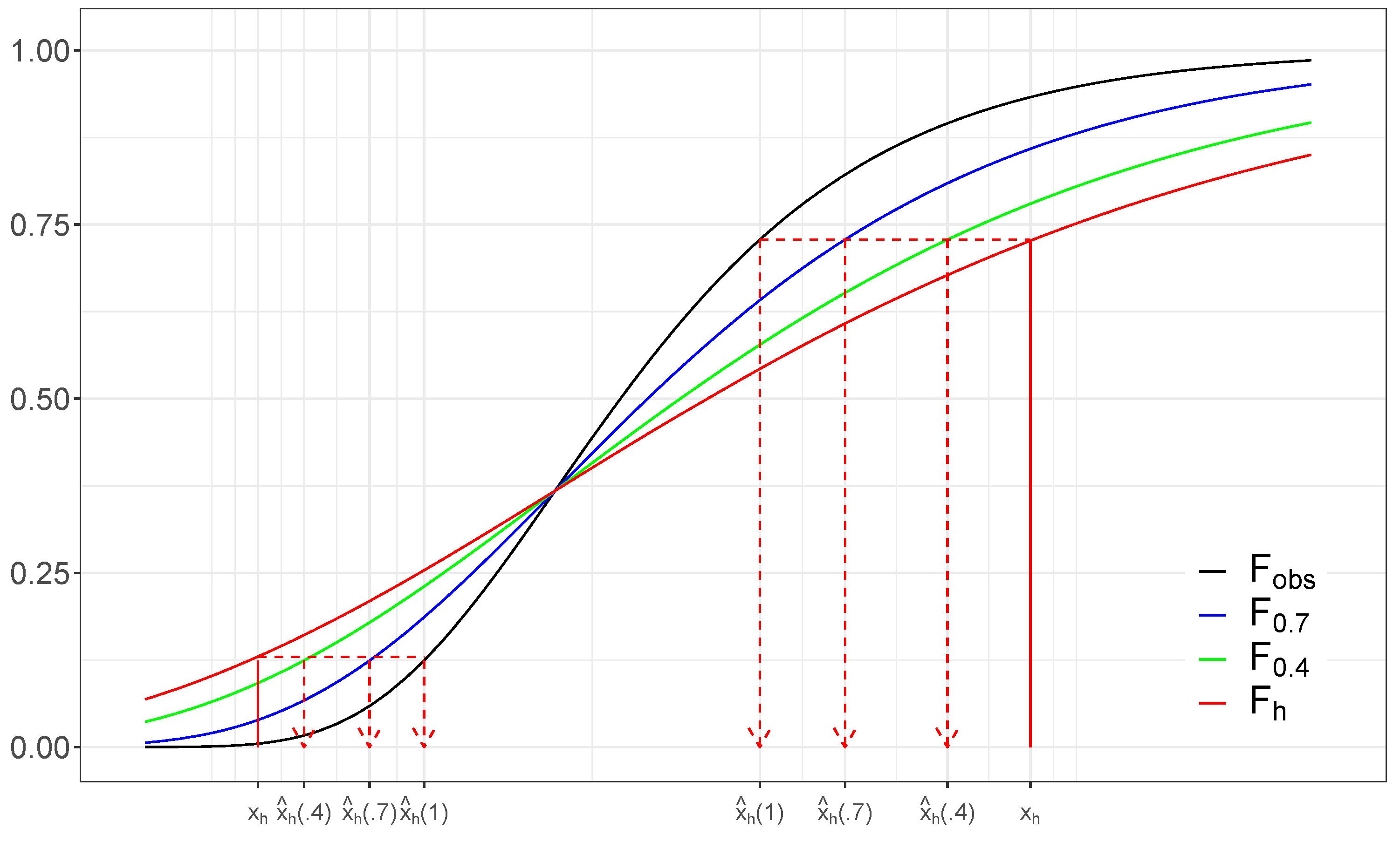
We refer (9) the “ α -correction” of the historical data to the observations. If α = 1 , then the α -correction is an ordinary QM. If α = 0 , then no BC is performed for the historical data. A sketch of the method with α = 0.4 and 0.7 is given in Figure 2. Note that x ^ h ( k ) ( 1 ) is not same as x o b s , but the cdf F 1 ( k ) from x ^ h ( k ) ( 1 ) is equal to F o b s for all k. The idea for the α -correction was inspired from examining various QM graphs in [48,49].

4.2. α -Weights

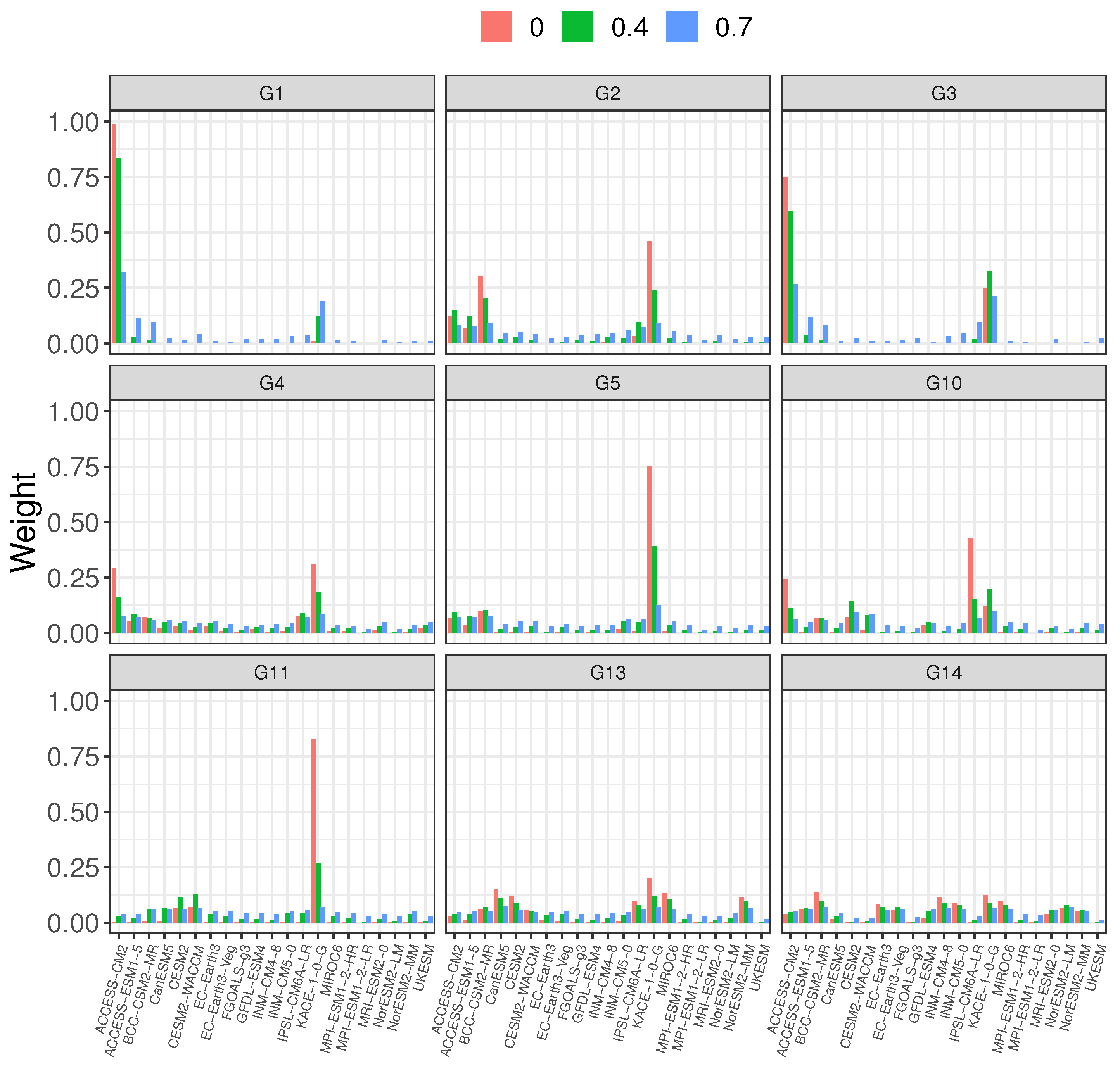
As α approaches 1, the BMA weights obtained from (3) become almost equal. When α = 0 , the usual BMA weights without any BC are obtained. In the latter case, sometimes a few excessively high weights dominate, while the remainder is very low (see Figure 3). If equal weights or a few dominating weights are undesirable, a hybrid one between these two situations may be an alternative. We expect that such hybrid weights can be obtained from the α -correction with a α value between 0 and 1, perhaps close to 0.5 . We call it “ α -weighting”, and denote the weights by w k ( α ) . See Figure 3 for the weights with α = 0 , 0.4 , and 0.7 , where a few very high weights for α = 0 decrease and few very low weights increase. The 0.4 -weights follow approximately the pattern of weights obtained by the original ( α = 0 ) BMA, whereas the 0.7 -weights go toward an even distribution. A figure depicting the the weights of additional α values is presented in the Supplementary Material.
Next, we describe the details of computing w k ( α ) . Here, to obtain the BMA weights or the α -weights, the historical data and observations are included without the future data. To obtain the α -weights in this study, we just followed the same procedure for calculating model weights as in the BMA, but with “nonzero” α .
We denote M k ( α ) as the α -corrected historical data of k-th model. The Gaussian likelihood is now modified to be dependent on α ; L ( M k ( α ) , T ) is the same as in (2) except that I i k ( T ) is replaced by I i k ( α , T ) , which is the intensity of the i-th bootstrap from the M k ( α ) . Then, we have the posterior probability of M k ( α ) for given the observations R :
p ( M k ( α ) | R ) = p ( R | M k ( α ) ) p ( M k ( α ) ) l = 1 K p ( R | M l ( α ) ) p ( M l ( α ) ) ,
where p ( R | M k ( α ) ) can be approximated by L ( M k ( α ) ) = 1 4 T L ( M k ( α ) , T ) as in [44], where 5, 10, 20, and 50 years are used for T in this study. Note that this averaged likelihood L ( M k ( α ) ) is actually a type of distance between G E V D ( R ) and G E V D ( M k ( α ) ) . When equal priors are given, the α -weights are
w k ( α ) = p ( M k ( α ) | R ) = L ( M k ( α ) ) l = 1 K L ( M l ( α ) ) .
The bias-corrected values in the future from the k-th model are obtained by the ordinary QM in our proposed method.
x ^ f ( k ) = F o b s 1 ( F h ( k ) ( x f ) ) .
The α -correction does not apply to the future data, but only to the past data to obtain the α -weights. The ensemble prediction for a quantity such as a 20-year return level ( r ^ 20 E ) in the future is obtained by
r ^ 20 E ( α ) = k = 1 K w k ( α ) r ^ 20 ( k ) ,
where r ^ 20 ( k ) is the 20-year return level estimated from the bias corrected future data ( x ^ f ( k ) ) for the k-th model. It should be noted that in (13), the quantity for r ^ 20 ( k ) does not depend on α (the result was obtained using α = 1 ).

4.3. Selection of the Correction Rate

Researchers may want to fix the α at one value. For this purpose, two methods applicable to each grid are presented here: The first method is the chi-square statistic for testing the null hypothesis of uniform (or equal) distribution of the weights, where H 0 : w k ( α ) = 1 / K for every k, and we let g k ( α ) = w k ( α ) × 100 . Then, for each grid, the chi-square statistic to test the above H 0 given by [38]
χ 0 2 ( α ) = k = 1 K ( g k ( α ) 100 / K ) 2 100 / K .
The values of g k ( α ) that are less than 5 are summed up to one category such that the total frequency is greater than 5. Let us denote K as the number of the categories that have the summed frequency greater than 5. If g k ( α ) are far from equal values, then χ 0 2 ( α ) will not be small. The null hypothesis is rejected at the 5% significance level when χ 0 2 ( α ) > χ 0.05 2 ( d f ) , where χ 0.05 2 ( d f ) is 95 percentile of a chi-square distribution with d f = K 1 degree of freedom.
There is more chance to reject H 0 for smaller α , and less chance to reject for α near to 1, because the α -weights become equal to each other as α goes up to 1. By changing the α from 0 to 1 in increments of 0.05, we can select the optimal α such that the null hypothesis is rejected, as follows,
α * = m a x 0 α 1 { α : χ 0 2 ( α ) > χ 0.05 2 ( d f ) } .
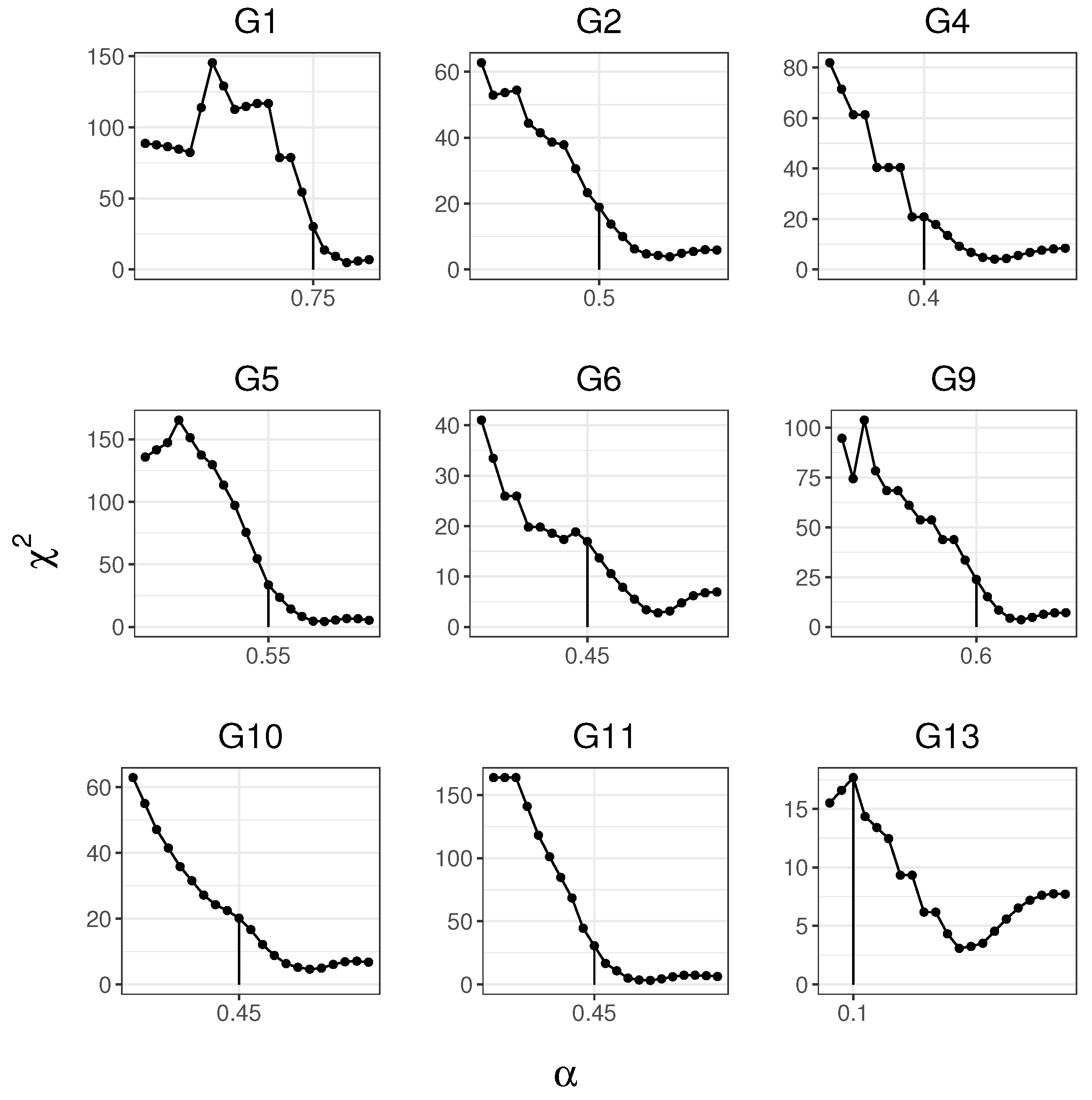
If there is no such α * in [0, 1], we set α * = 0 . As this selection is done for each grid cell, the α * value is determined independently for each cell. Figure 4 shows the chi-square test statistics calculated from various α -weights and the selected optimal α j * for select j-th grid cell.
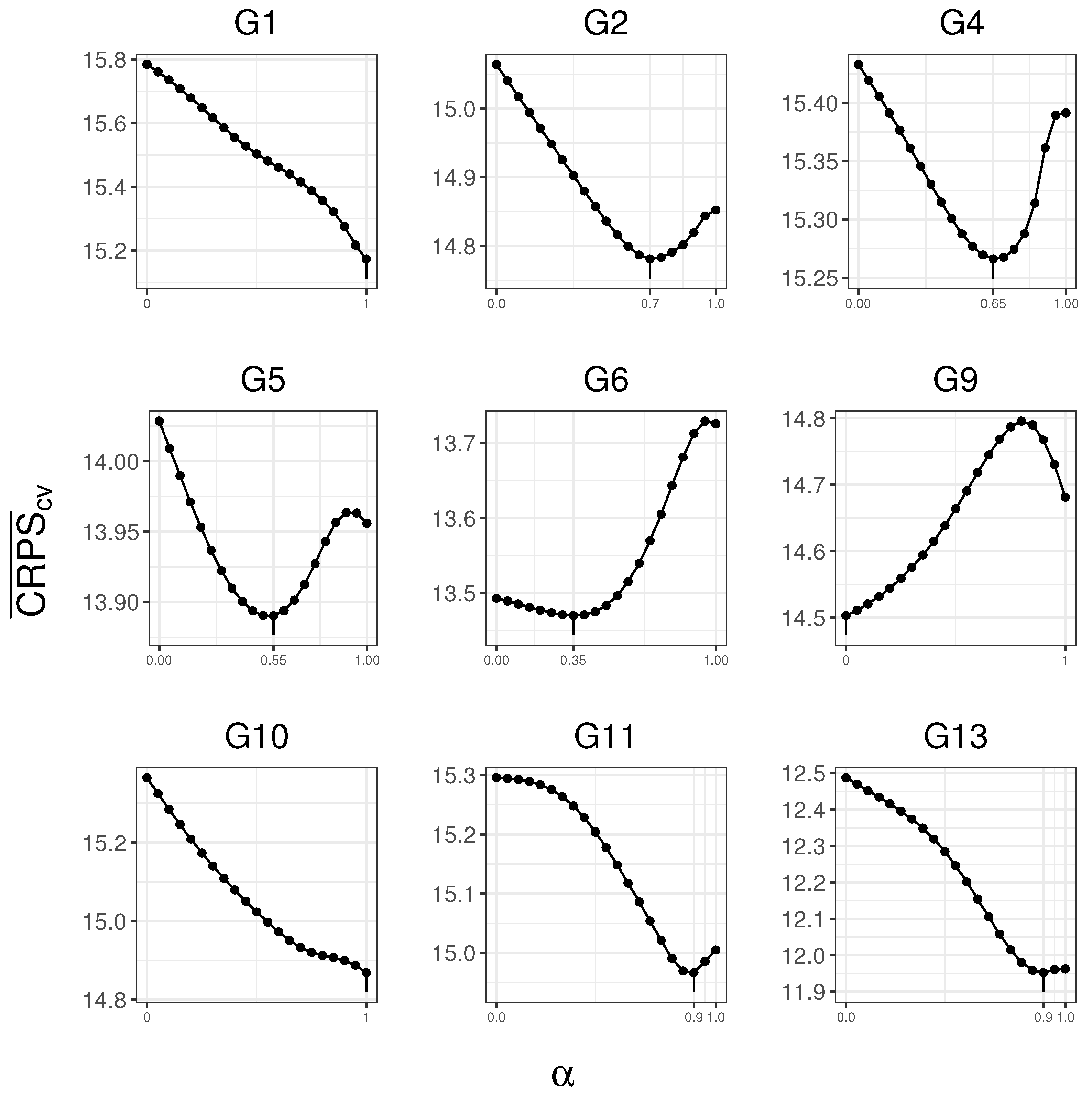
As another way of selecting an optimal α , we consider the use of the continuous ranked probability score (CRPS), which can be employed to evaluate the impact of the weighting on the skill of the future projections. The CRPS defined for a single forecast can be extended for multiple occasions by averaging it, which is detailed in [50]. The averaged CRPS can be formulated as a function of α -weights, denoted by C R P S ¯ ( α ) . In the next section, the leave-one-model-out version is averaged to compute C R P S ¯ c v ( α ) as in Equation (16). Thus, an optimal α can be chosen at the minimum of the C R P S ¯ c v ( α ) . These optimal α j s values, selected differently from each grid, can lead to an increase in skill while minimizing the probability of overfitting [27]. In selecting an appropriate α , one can consider other criterion such as entropy [19] or the cross-validated mean squared error.
Figure 5 shows the selected optimal α j and the values of C R P S ¯ c v ( α ) as α increases from 0 to 1 for each j-th grid. More figures for different future periods and scenarios are available in the Supplementary Material.
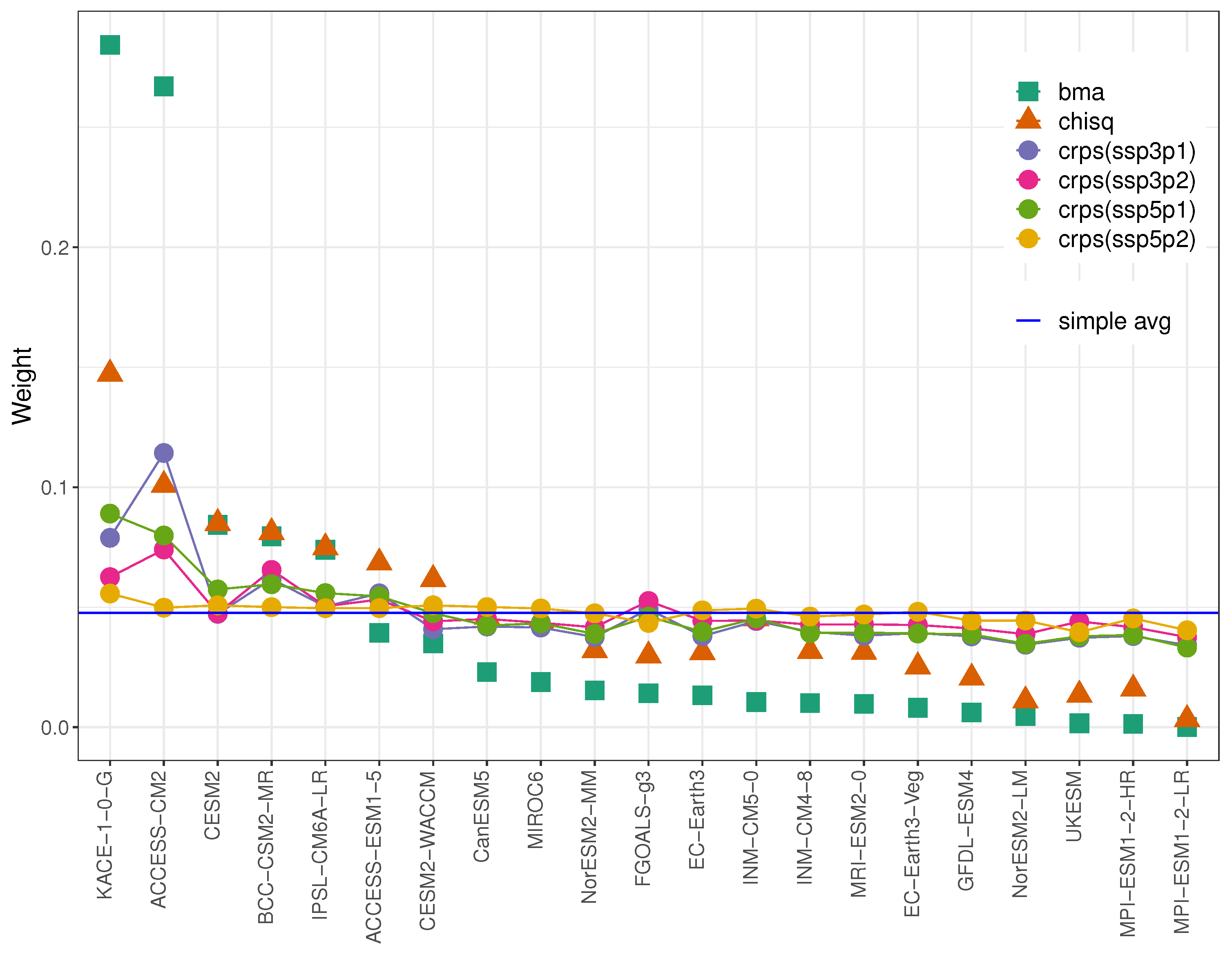
Figure 6 shows the weights for 21 models obtained from various α -weighting methods. We see that two high weights from BMA decrease significantly, while most small weights increase slightly by the α -correction methods. It seems that the methods based on C R P S alter the weights by bringing them closer to equal in value. The α selection method based on the chi-square statistic is relatively easier to computate and it smooths the BMA weights well, but may lack climatological meaning. The method based on the C R P S has a clear climatological meaning, but for this study at least, shifts the weights towards being different in value.
Instead of using one set of weights, one can apply several sets of weights that are obtained from various values of α . For example, α can be set to 0, 0.25, 0.5, 0.75, and 1. Several different prediction results from such α values are available. These multiple results provide various plausible shapes of the future climate change which may not be detected by a single ensemble.

5. Comparison of Weighting Schemes

Some metrics can be used to compare weighting schemes and assess the skill of “out-of-sample” ensemble prediction. Those metrics include absolute error, ensemble spread, overconfidence bias, and ranked probability skill score [30]. The latter is based on C R P S ¯ and is essentially a combination of accuracy (absolute error of prediction) and precision (the width of predictive distribution) [30]. These are computed under the following models-as-truth experiments. In this study, however, we consider only C R P S ¯ c v ( α ) as a metric.

5.1. Leave-One-Model-Out Validation

This approach picks each model from a multi-model ensemble in turn and treats it as the true representation of the climate system. The data from this perfect model are treated as true observations, termed as “pseudo-observations”. Then, the α -weights are obtained by following the same process presented in the above Section 4.2. Actually, the pseudo-observations from the perfect model and the α -corrected historical data for the remaining models are used. This leave-one-model-out method is called a model-as-truth experiment or a perfect model test [27,30]. This allows for an evaluation of the impact of the weighting in the future based on each model representing the truth once.
As a measure of the method’s skill, we use the C R P S ¯ ( α ) as mentioned in the above section. Here, the leave-one-model-out cross-validated version, C R P S ¯ ( k ) ( α ) , is employed. This is basically the average of the mean squared error between the distribution of the k-th perfect model and the distribution of all other models except for the k-th model [27]. The distribution of all other models is composed of α -weighted average of the distributions of the K 1 models. Then, the C R P S ¯ c v ( α ) is averaged over the K models as. Thus,
C R P S ¯ c v ( α ) = 1 K k = 1 K C R P S ¯ ( k ) ( α ) .
Small values for this quantity may represent a better performance in projecting future climate. For numerical computation, we used the “scoringRules” package in R [51].
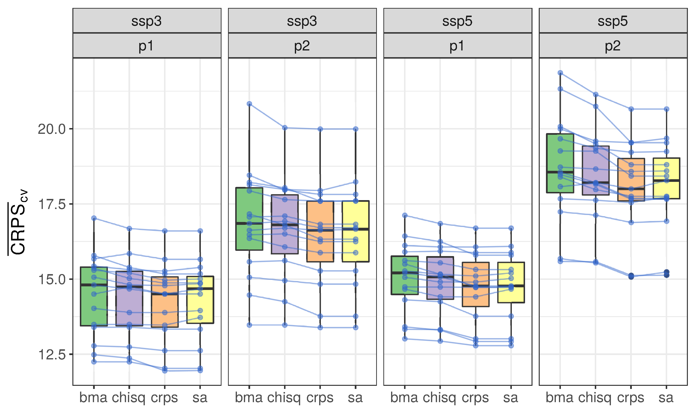
Figure 7 shows parallel coordinated box-plots of C R P S ¯ c v ( α ) calculated over 15 grid cells for future periods P1 and P2 under both SSP3 and SSP5 scenarios. The details of the parallel coordinated box-plots are described in the Supplementary Material. The optimal α -weights based on C R P S ¯ c v ( α ) produces the best performance among those considered in this study. Its performances in P2 of the SSP3 scenario and P1 of the SSP5 scenario are, however, similar to those of the simple average. This is because the selected optimal α s based on the C R P S are equal to 1 in many of the grid cells. In addition, we see that the chi-square-based approach works better than the BMA.
The C R P S ¯ ( k ) ( α ) can be interpreted as the difficulty in predicting the k-th model from all other K 1 models. When its value is small, the k-th model is more explicable by a combination of other K 1 models than when it is large. Considering this, it is notable that the C R P S values for P2 (SSP5) are greater than those for P1 (SSP3) in Figure 7. This may mean that the mutual predictability or the coherence among the models is weaker for the far future and the SSP5 scenario than those for the near future and the SSP3.
In calculating the LOOCV based on C R P S on 15 grid cells for 21 models, we experienced too much computing time, as α changes from 0 to 1 by 0.05. It took more than 120 min on an Intel i5 PC with 16 GB memory. Therefore, a parallel computing using “foreach” package [52] in R program was executed on a GPU server (Xeon*G 6230) with 80 cores. It took approximately 5 min. When the study region gets wider or the number of grid cells are large for several weather variables and for more than 21 models in CMIP6, it seems the parallel computing is necessary. In the sense of computing time only, selection of the correction rate based on the chi-square statistic may be preferred to that based on C R P S with a perfect model test.

5.2. Quantile Estimation

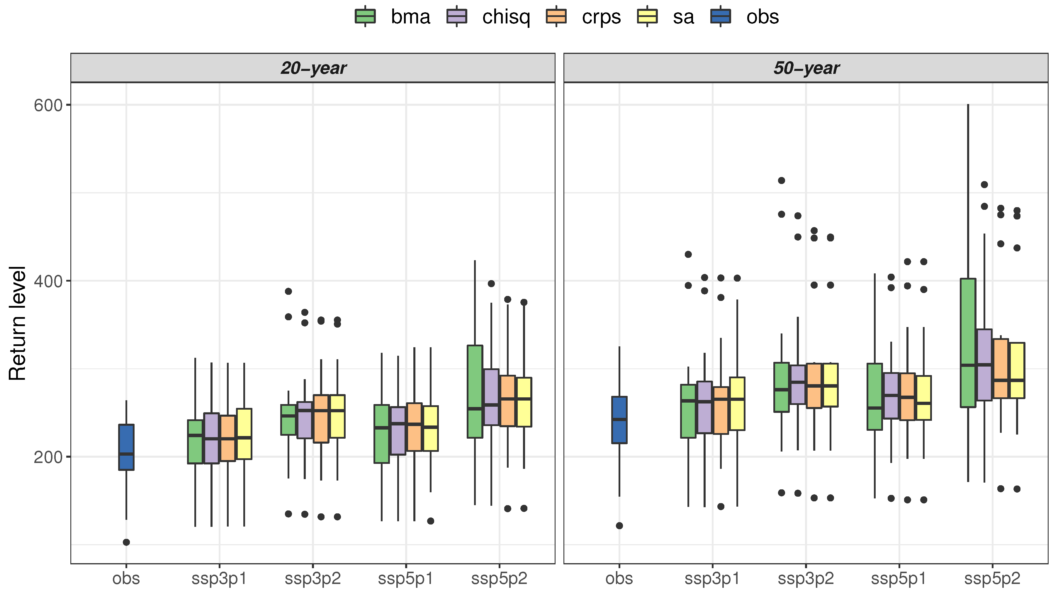
Figure 8 shows schematic box-plots of the 20- and 50-year return levels of the annual maximum daily precipitation for 15 grid cells over the Korean peninsula obtained from various α -weights based on the BMA, the chi-square statistic, the C R P S , and the simple averaging (SA). Compared to the observations, the return levels for all cases increase in the future; more in P2 and the SSP5 scenario than in P1 and the SSP3, respectively. Figure 9 depicts the similar plots as Figure 8 but for 20- and 50-year return periods (i.e., waiting time) relative to the observations from 1973 to 2014.
The results from Figure 7, Figure 8 and Figure 9 show the differences due to the weighting schemes, but the differences may not be as distinctive as they appear. Because the results from the weighted and unweighted means are similar, one may question why the simple average could not be used. Lorenz et al. [29] argued that although the resulting numbers may be similar, the interpretation of the spread is different between the unweighted and the weighted multi-model means. In that paper, they wrote the following. “The spread of the simple average is just a spread and is not a measure of uncertainty. It is an ad hoc measure of spread reflecting the ensemble design, or lack thereof, whereas the spread in the weighted multi-model mean can be interpreted as a measure of uncertainty given everything we know. We thus should have more confidence in the latter”.
Plots in Figure 9 indicate that the 20-year return periods for P2 are about 0.75 times shorter than those for P1. Specially, the 20-year return period for P2 under the SSP5 is very short, about 7 years in median. By reading the right-hand plots too, we realize that a 1-in-20 year (1-in-50 year) annual maximum daily precipitation in the Korean peninsula will likely become a 1-in-10 (1-in-20) year and a 1-in-7 (1-in-15) year event in median by the end of the 21st century based on the SSP3 (the SSP5) scenarios, respectively, when compared to the observation from 1973 to 2014. These show that the 20-year and 50-year return periods will likely reduce to approximately half (40%) under the SSP3 scenario and approximately one-third (30%) under SSP5 by the end of the 21st century. This is approximately of equal frequency as that in the result by Lee et al. [25], which was obtained by a multi-model ensemble with the BMA weights based on 17 CMIP5 simulation models. They showed that both 20- and 50-year return periods across the Korean peninsula will likely reduce to approximately half for RCP 4.5 and to approximately one-quarter for RCP 8.5 by the end of the 21st century, compared to the observations from 1971 to 2005.

6. Discussion

The idea of the α -correction based on QM proposed in this paper is only based only on the at-site BC, which may be unreasonable and, and therefore is a limitation of this approach. The α -correction can be applied to the BC based on some variants of QM [14]. The variation of the C R P S ¯ c v ( α ) values among the grid cells is larger than those among various α -weights, as seen in Figure 5. This high variation among grid cells may be reduced by using the regional BC, which takes into account the spatial dependence between nearby grids. Some multivariate spatial BC methods [16,46] with the α -correction may lead to reduce uncertainty, consideration of spatial pattern or correlation, and to increased skill of ensembles more than an at-site BC.
Ensembles from various sets of α -weights can be recombined to produce another ensemble. This ensemble of ensembles is referred to the double ensemble (DE) or stacking [36]. If there are L number of ensembles in which each ensemble is constructed from a set of α l -weights, for l = 1 , , L , the prediction is a form of I ^ D E = l = 1 L v ( α l ) I ^ ( α l ) , where v ( α l ) is another weight for the l-th ensemble, and I ^ ( α l ) is the predicted value from the l-th ensemble with a set of α l . One can choose α l = 0 , 0.5 , 1 or α l = 0 , 1 / 4 , 0.5 , 3 / 4 , 1 for simple examples. In this case, the selection of a specific α is no longer required. As another example, in addition to α l = 0 , 1 , one can include the ensembles with α 1 * and α 2 * , which are the optimal correction rates obtained by the chi-square test statistic and by the C R P S ¯ c v ( α ) , respectively, for each grid cell. It is known that this DE generally leads to better prediction than a single ensemble in the sense of reducing the variance [36], but this requires more computational efforts. Equal values can be set to v ( α l ) for a simple average calculation. One may assign different values for v ( α l ) based on a cross-validated criterion as in statistical learning.
The leave-one-out (LOO) cross-validation (CV) based on C R P S was employed in this study to find an optimal correction rate and to compare weighting schemes. The LOOCV perfect model test and the model-as-truth experiment have been used to select hyperparameters in the weights and to evaluate the weighting scheme, respectively, in multi-model ensemble studies [6,27,29,37]. In the statistical learning community, however, the k-fold CV is preferred over LOOCV due to the higher variance of LOOCV, than does that of k-fold CV [36]. The k-fold CV approach involves randomly dividing the set of models into k groups or folds of approximately same size. The first fold is treated as a validation set, and the method calculates the C R P S ( 1 ) based on the remaining k 1 folds. This is repeated for all k-folds; each time, a different fold is treated as a validation set. It finally produces the averaged value C R P S ¯ c v similarly to a formula in Equation (16). LOOCV is a special case of k-fold CV in which k is set to equal the number (K) of models. In practice, one can perform k-fold CV using k = 5 or k = 10 (when K is large). LOOCV is not involved with randomness, whereas the k-fold CV is dependent on random divisions of models into k groups. The latter approach requires further considerations to be applicable to the weighting scheme in the multi-model climate ensemble study. If we employed the k-fold CV instead of LOOCV in the above section, the results might be altered.
The weights in the BMA employed in this study are obtained based on the performance of the model. The performance is defined by the distance between the historical data and the observations, which measures how well the model reproduces the historical data close to the observations. This performance, however, may not guarantee the reliability of future climate change. In some cases, nonetheless, past trends are strongly related to future trends, e.g., for large-scale greenhouse gas-induced warming [53] or Arctic sea ice decline [54]. The study by Smith and Chandler [55] in this issue shows that present-day climate and variability are related to the predicted change in precipitation in parts of Australia [21]. Therefore, a performance criterion based on the distance between the historical data and the observations may be necessary in calculating the model weights, but is not sufficient. In addition to the performance measure, one can include others such as uncertainties in the model or in the observations, the model convergence criterion [1], or the model independence [5,6]. The α -weighting proposed in this study is related to uncertainties in data. Large uncertainties in the model or in the observations weaken the confidences on the model performance and on the weights based on the performance. We can infer that the weights in this situation are determined by more chance than in the situation with lower uncertainties. Especially, a few models with very high weights which dominate most other models with very low weights would be unfair and may result in an unreliable and unrobust prediction. The method in this study was thus proposed to smooth or regulate such weights.
If we have another set of weights, for instance, d m , such as for the independence of the m-th model, then a new weighting scheme of combining both weights is obtained by, for m = 1 , , K ,
u m ( α ) = w m ( α ) d m l = 1 K w l ( α ) d l .
This approach can lead to a weighting scheme accounting for performance and independence simultaneously [5,6,27].
One can further consider the α -weighting to the future model data too. It may introduce another “semi”-bias correction, which adds complexity to the situation. Nevertheless, this would enrich the methodology of ensemble prediction. We leave this undertaking future work.

7. Conclusions

Multi-model ensemble methods in climatic projection have proved to improve upon the systematic bias and general limitations of a single simulation model. It has been argued that model uncertainty can be reduced by attributing more weight to those models that are more skillful and realistic for a specific process or application. As both bias-correction (BC) and model weighting are common procedure in impact studies, we considered a weighting scheme that includes both equal and unequal weights for a bias-corrected simulation model output. The proposed approach applies an “imperfect” BC or α -correction to the historical data in computing the model weights, while it applies ordinary BC to the future data in computing the weighted average for projection.
The proposed weighting scheme prevents the situation where only a few models have very high weights and the most majority have very low weights, which frequently occurs in the BMA approach. Our method, conversely, seeks to shift the high weights far from those that are equal. It, therefore, searches for a balanced “sweet spot” between BMA weights and simple averaging. A weighting scheme in which an optimal correction rate is selected based on the chi-square test statistic smooths unfairly high or low weights, while it continues to reject the hypothesis of the uniform distribution.
Based on this generalized or hybrid scheme, researchers can present their optimal results between equal and BMA weights. We illustrated from model-as-truth experiments that an ensemble with a set of weights obtained by minimizing the C R P S ¯ c v ( α ) can improve the skill to a greater extent than the BMA and simple averaging. One may provide multiple results from several weighted ensembles to capture various plausible shapes and uncertainties of future changes.
The numerical results and the selected α s illustrated here using the annual maximum daily precipitation in the Korean peninsula depend strongly on variables, regions, and simulation model outputs. The introduction of α -correction and α -weights, however, is a step that can serve to combine simulation models optimally and with more flexibility. A more refined α -weights method, such as the one we developed in this study, can deserve to be included in a discourse about tactics to build a better multi-model ensemble in predicting future climate.

Supplementary Materials

The following are available online at https://www.mdpi.com/2073-4433/11/8/775/s1, Figure S1: Distributions of the weights obtained from various α -corrections for each grid cell. Red, green, and blue bars represent the α -weights with α = 0 , 0.4 , 0.7 , respectively. Figure S2: Distributions of the weights obtained from various α -corrections for each grid cell. Red, green, and blue bars represent the α -weights with α = 0.2 , 0.5 , 0.8 , respectively. Figure S3: Plots of the chi-square test statistics as α changes from 0 to 1, and the selected optimal correction rate α * for 15 grid cells. Figure S4: Computed values of C R P S ¯ c v ( α ) defined as in Equation (16) and the selected optimal correction rate α for 15 grid cells and for the future period 1 (2021–2060) under the SSP3 scenario. Figure S5: Same as Figure S4 but for the future period 2 (2061–2100) under the SSP3 scenario. Figure S6: Same as Figure S4 but for the future period 1 (2021–2060) under the SSP5 scenario. Figure S7: Same as Figure S4 but for the future period 2 (2061–2100) under the SSP5 scenario.

Author Contributions

Conceptualization, Y.L. and J.-S.P.; methodology, Y.L.; software, Y.S.; validation, Y.S. and Y.L.; formal analysis, Y.S. and Y.L.; investigation, Y.S. and Y.L.; resources, Y.S. and Y.L.; data curation, Y.S.; writing—original draft preparation, J.-S.P.; writing—review and editing, Y.L.; visualization, Y.S.; supervision, Y.L.; project administration, J.-S.P.; funding acquisition, J.-S.P. All authors have read and agreed to the published version of the manuscript.

Funding

This study was supported by the National Research Foundation of Korea (NRF) grant funded by the Korea government (No. 2020R1I1A3069260) and funded by the Korea Meteorological Administration Research and Development Program under Grant KMI2018-03414.

Acknowledgments

The authors would like to thank the reviewers and the guest editors of the special issue for helpful comments and suggestions, which have greatly improved the presentation of this paper. We acknowledge the World Climate Research Programme Working Group on Coupled Modelling, which is responsible for CMIP, and we thank the climate modeling groups for producing and making available their model output. For CMIP, the U.S. Department of Energy Program for Climate Model Diagnosis and Intercomparison provides coordinating support and led the development of software infrastructure in partnership with the Global Organization for Earth System Science Portals. We thank all contributors to the numerical R packages which were crucial for this work. The authors are also grateful to Juyoung Hong for collecting data and for administrative management on research grant.

Conflicts of Interest

The authors declare no conflict of interest.

References

  1. Georgi, F.; Mearns, L.O. Calculation of average, uncertainty range and reliability of regional climate changes from AOGCM simulations via the ‘Reliability Ensemble Averaging (REA)’ method. J. Clim. 2002, 15, 1141–1158. [Google Scholar] [CrossRef]
  2. Tebaldi, C.; Knutti, R. The use of multi-model ensemble in probabilistic climate projections. Phil. Trans. R. Soc. A 2007, 365, 2053–2075. [Google Scholar] [CrossRef] [PubMed]
  3. Smith, R.L.; Tebaldi, C.; Nychka, D.; Mearns, L.O. Bayesian modeling of uncertainty in ensembles of climate models. J. Am. Stat. Assoc. 2009, 104, 97–116. [Google Scholar] [CrossRef]
  4. Coppola, E.; Giorgi, F.; Rauscher, S.; Piani, C. Model weighting based on mesoscale structures in precipitation and temperature in an ensemble of regional climate models. Clim. Res. 2010, 44, 121–134. [Google Scholar] [CrossRef] [Green Version]
  5. Sanderson, B.M.; Knutti, R.; Caldwell, P. A representative democracy to reduce interderpendency in a multimodel ensemble. J. Clim. 2015, 28, 5171–5194. [Google Scholar] [CrossRef] [Green Version]
  6. Knutti, R.; Sedlacek, J.; Sanderson, B.M.; Lorenz, R.; Fischer, E.M.; Eyring, V. A climate model projection weighting scheme accounting for performance and independence. Geophys. Res. Lett. 2017, 44, 1909–1918. [Google Scholar]
  7. Hoeting, J.A.; Madigan, D.; Raftery, A.E.; Volinsky, C.T. Bayesian model averaging: A tutorial. Stat. Sci. 1999, 14, 382–417. [Google Scholar]
  8. Raftery, A.E.; Gneiting, T.; Balabdaoui, F.; Polakowski, M. Using Bayesian model averaging to calibrate forecast ensembles. Mon. Weather Rev. 2005, 133, 1155–1174. [Google Scholar] [CrossRef] [Green Version]
  9. Sloughter, J.M.; Raftery, A.E.; Gneiting, T.; Fraley, C. Probabilistic quantitative precipitation forecasting using Bayesian model averaging. Mon. Weather Rev. 2007, 135, 3209–3220. [Google Scholar] [CrossRef]
  10. Darbandsari, P.; Coulibaly, P. Inter-comparison of different Bayesian model averaging modifications in streamflow simulation. Water 2019, 11, 1707. [Google Scholar] [CrossRef] [Green Version]
  11. Sanderson, B.M.; Knutti, R.; Caldwell, P. Addressing interdependency in a multimodel ensemble by interpolation of model properties. J. Clim. 2015, 28, 5150–5170. [Google Scholar] [CrossRef]
  12. Coles, S. An Introduction to Statistical Modelling of Extreme Values; Springer: New York, NY, USA, 2001; p. 224. [Google Scholar]
  13. Zhu, J.; Forsee, W.; Schumer, R.; Gautam, M. Future projections and uncertainty assessment of extreme rainfall intensity in the United States from an ensemble of climate models. Clim. Chang. 2013, 118, 469–485. [Google Scholar] [CrossRef]
  14. Maraun, D.; Widmann, M. Statistical Downscaling and Bias Correction for Climate Research; Cambridge University Press: Cambridge, UK, 2018. [Google Scholar]
  15. Wehner, M.F.; Easterling, D.R.; Lawrimore, J.H.; Heim, R.R., Jr.; Vose, R.S.; Santer, B. Projections of future drought in the continental United States and Mexico. J. Hydrometeorol. 2011, 12, 1359–1377. [Google Scholar] [CrossRef]
  16. Cannon, A.J. Multivariate quantile mapping bias correction: An N-dimensional probability density function transform for climate model simulations of multiple variables. Clim. Dyn. 2018, 50, 31–49. [Google Scholar] [CrossRef] [Green Version]
  17. Brekke, L.D.; Barsugli, J.J. Uncertainties in projections of future changes in extremes. In Extremes in a Changing Climate: Detection, Analysis and Uncertainty; AghaKouchak, A., Eatering, D., Hsu, K., Schubert, S., Sorooshian, S., Eds.; Springer: Dordrecht, The Netherlands, 2013. [Google Scholar]
  18. Annan, J.D.; Hargreaves, J.C. Reliability of the CMIP5 ensemble. Geophys. Res. Lett. 2010, 37, L02703. [Google Scholar] [CrossRef]
  19. Wang, H.M.; Chen, J.; Xu, C.Y.; Chen, H.; Guo, S.; Xie, P.; Li, X. Does the weighting of climate simulation result in a better quantification of hydrological impacts? Hydrol. Earth Syst. Sci. 2019, 23, 4033–4050. [Google Scholar] [CrossRef] [Green Version]
  20. Stainforth, D.A.; Allen, M.R.; Tredger, E.R.; Smith, L.A. Confidence, uncertainty and decision-support relevance in climate predictions. Philos. Trans. R. Soc. A 2007, 365, 2145–2161. [Google Scholar] [CrossRef]
  21. Knutti, R. The end of model democracy? Clim. Chang. 2010, 102, 394–404. [Google Scholar] [CrossRef]
  22. Massoud, E.C.; Espinoza, V.; Guan, B.; Waliser, D.E. Global Climate Model Ensemble Approaches for Future Projections of Atmospheric Rivers. Earth’s Future 2019, 7, 1136–1151. [Google Scholar] [CrossRef] [Green Version]
  23. Wenzel, S.; Cox, P.M.; Eyring, V.; Friedlingstein, P. Emergent constraints on climate-carbon cycle feedbacks in the CMIP5 Earth system models. J. Geophys. Res. Biogeosci. 2014, 119, 794–807. [Google Scholar] [CrossRef] [Green Version]
  24. Eyring, V.; Cox, P.M.; Flato, G.M.; Gleckler, P.J.; Abramowitz, G.; Caldwell, P.; Collins, W.D.; Gier, B.K.; Hall, A.D.; Hoffman, F.M.; et al. Taking climate model evaluation to the next level. Nat. Clim. Chang. 2019, 9, 102–110. [Google Scholar] [CrossRef] [Green Version]
  25. Lee, Y.; Shin, Y.G.; Park, J.S.; Boo, K.O. Future projections and uncertainty assessment of precipitation extremes in the Korean peninsula from the CMIP5 ensemble. Atmos. Sci. Lett. 2020, e954. [Google Scholar] [CrossRef] [Green Version]
  26. Xu, D.; Ivanov, V.; Kim, J.; Fatichi, S. On the use of observations in assessment of multi-model climate ensemble. Stoch. Environ. Res. Risk Assess. 2019, 33, 1923–1937. [Google Scholar] [CrossRef]
  27. Brunner, L.; Lorenz, R.; Zumwald, M.; Knutti, R. Quantifying uncertainty in European climate projections using combined performance-independence weighting. Environ. Res. Lett. 2019, 14, 124010. [Google Scholar] [CrossRef]
  28. Abramowitz, G.; Gupta, H. Toward a model space and model independence metric. Geophy. Res. Lett. 2008, 35, L05705. [Google Scholar] [CrossRef] [Green Version]
  29. Lorenz, R.; Herger, N.; Sedlacek, J.; Eyring, V.; Fischer, E.M.; Knutti, R. Prospects and caveats of weighting climate models for summer maximum temperature projections over North America. J. Geophys. Res. Atmos. 2018, 123, 4509–4526. [Google Scholar] [CrossRef]
  30. Herger, N.; Abramowitz, G.; Sherwood, S.; Knutti, R.; Angelil, O.; Sisson, S. Ensemble optimisation, multiple constrints and overconfidence: A case study with future Australian precipitation change. Clim. Dyn. 2019. [Google Scholar] [CrossRef]
  31. O’Neill, B.C.; Kriegler, E.; Riahi, K.; Ebi, K.L.; Hallegatte, S.; Carter, T.R.; Mathur, R.; van Vuuren, D.P. A new scenario framework for climate change research: The concept of Shared Socioeconomic Pathways. Clim. Chang. 2014, 122, 387–400. [Google Scholar] [CrossRef] [Green Version]
  32. Koch, S.E.; DesJardins, M.; Kocin, P.J. An interactive Barnes objective map analysis scheme for use with satellite and conventional data. J. Clim. Appl. Meteorol. 1983, 22, 1487–1503. [Google Scholar] [CrossRef]
  33. Maddox, R.A. An objective technique for separating macroscale and mesoscale features in meteorological data. Mon. Weather Rev. 1980, 108, 1108–1121. [Google Scholar] [CrossRef] [Green Version]
  34. Kuleshov, Y.; de Hoedt, G.; Wright, W.; Brewster, A. Thunderstorm distribution and frequency in Australia. Aust. Meteorol. Mag. 2002, 51, 145–154. [Google Scholar]
  35. Garcia-Pintado, J.; Barbera, G.G.; Erena, M.; Castillo, V.M. Rainfall estimation by rain gauge-radar combination: A concurrent multiplicative-additive approach. Water Resour. Res. 2009, 45, W01415. [Google Scholar] [CrossRef]
  36. Hastie, T.; Tibshirani, R.; Friedman, J. The Elements of Statistical Learning, 2nd ed.; Springer: Berlin/Heidelberg, Germany, 2009. [Google Scholar]
  37. Abramowitz, G.; Bishop, C.H. Climate model dependence and the ensemble dependence transformation of CMIP projections. J. Clim. 2015, 28, 2332–2348. [Google Scholar] [CrossRef]
  38. Wilks, D. Statistical Methods in the Atmospheric Sciences, 3rd ed.; Academic Press: New York, NY, USA, 2011. [Google Scholar]
  39. Hosking, J.R.M.; Wallis, J.R. Regional Frequency Analysis: An Approach Based on L-Moments; Cambridge University Press: Cambridge, UK, 1997; p. 244. [Google Scholar]
  40. Hosking, J.R.M. L-Moments. R Package, Version 2.8. 2019. Available online: https://CRAN.R-project.org/package=lmom (accessed on 28 May 2020).
  41. Niu, X.; Wang, S.; Tang, J.; Lee, D.K.; Gutowsky, W.; Dairaku, K.; McGregor, J.; Katzfey, J.; Gao, X.; Wu, J.; et al. Ensemble evaluation and projection of climate extremes in China using RMIP models. Int. J. Climatol. 2018, 38, 2039–2055. [Google Scholar] [CrossRef]
  42. Qi, H.; Zhi, X.; Peng, T.; Bai, Y.; Lin, C. Comparative Study on Probabilistic Forecasts of Heavy Rainfall in Mountainous Areas of the Wujiang River Basin in China Based on TIGGE Data. Atmosphere 2019, 10, 608. [Google Scholar] [CrossRef] [Green Version]
  43. Sun, H.; Yang, Y.; Wu, R.; Gui, D.; Xue, J.; Liu, Y.; Yan, D. Improving Estimation of Cropland Evapotranspiration by the Bayesian Model Averaging Method with Surface Energy Balance Models. Atmosphere 2019, 10, 188. [Google Scholar] [CrossRef] [Green Version]
  44. Rojas, R.; Feyen, L.; Dassargues, A. Conceptual model uncertainty in groundwater modeling: Combining generalized likelihood uncertainty estimation and Bayesian model averaging. Water Resour. Res. 2008, 44, W12418. [Google Scholar] [CrossRef] [Green Version]
  45. Christensen, J.H.; Boberg, F.; Christensen, O.B.; Lucas-Picher, P. On the need for bias correction of regional climate change projections of temperature and precipitation. Geophys. Res. Lett. 2008, 35, L20709. [Google Scholar] [CrossRef]
  46. Vrac, M.; Friederichs, P. Multivariate-intervariable, spatial, and temporal-bias correction. J. Clim. 2015, 28, 218–237. [Google Scholar] [CrossRef]
  47. Panofsky, H.; Brier, G. Some Applications of Statistics to Meteorology; Pennsylvania State University: University Park, PA, USA, 1968; p. 224. [Google Scholar]
  48. Switanek, M.B.; Troch, P.A.; Castro, C.L.; Leuprecht, A.; Chang, H.I.; Mukherjee, R.; Demaria, E. Scaled distribution mapping: A bias correction method that preserves raw climate model projected changes. Hydrol. Earth Syst. Sci. 2015, 21, 2649–2666. [Google Scholar] [CrossRef] [Green Version]
  49. Pierce, D.W.; Cayan, D.R.; Maurer, E.P.; Abatzoglou, J.T.; Hegewisch, K.C. Improved bias correction techniques for hydrological simulations of climate change. J. Hydrometeorol. 2015, 16, 2421–2442. [Google Scholar] [CrossRef]
  50. Hersbach, H. Decomposition of the continous ranked probability score for ensemble prediction systems. Weather Forecast 2000, 15, 559–570. [Google Scholar] [CrossRef]
  51. Jordan, A.; Krüger, F.; Lerch, S. Evaluating probabilistic forecasts with scoringRules. J. Stat. Softw. 2018, 90, 1–37. [Google Scholar] [CrossRef] [Green Version]
  52. Calaway, R.; Ooi, H.; Weston, S. Package ‘Foreach’. R Program Repository CRAN. 2020. Available online: https://github.com/RevolutionAnalytics/foreach (accessed on 28 May 2020).
  53. Scott, P.A.; Kettleborough, J.A. Origins and estimates of uncertainty in predictions of twenty-first century temperature rise. Nature 2002, 416, 723–726. [Google Scholar]
  54. Boe, J.L.; Hall, A.; Qu, X. September sea-ice cover in the Arctic Ocean projected to vanish by 2100. Nat. Geosci. 2009, 2, 341–343. [Google Scholar] [CrossRef]
  55. Smith, I.; Chandler, E. Refining rainfall projections for the Murray Darling Basin of south-east Australia–the effect of sampling model results based on performance. Clim. Chang. 2010, 102, 377–393. [Google Scholar] [CrossRef]
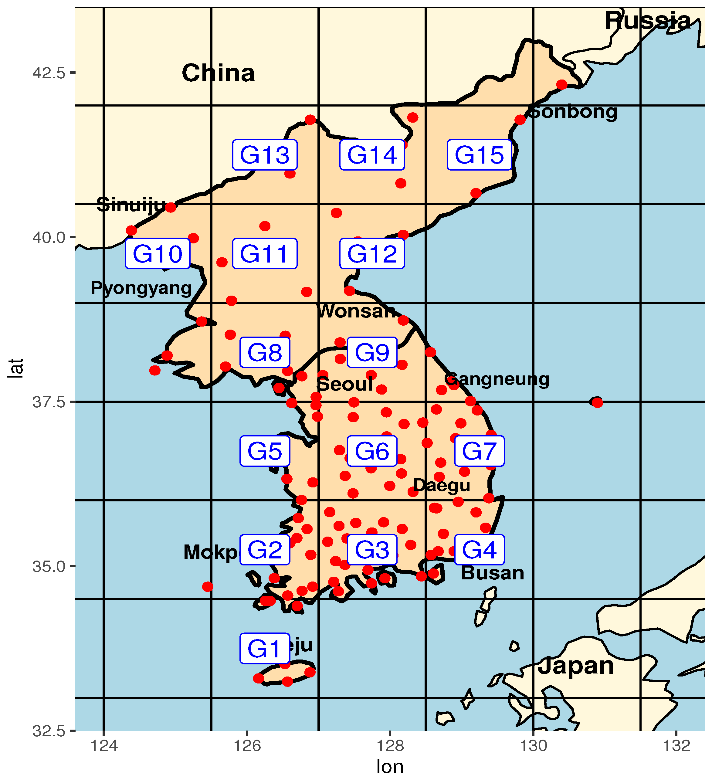
Figure 1. Map of the Korean peninsula, the spatial distribution of 127 rainfall observed stations, and 15 grid cells used in this study.
Atmosphere 11 00775 g001
Figure 2. A sketch of quantile mapping with various α -corrections, where the historical simulated cumulative distribution function (cdf)( F h ) is mapped onto the α -corrected cdfs. F o b s is the cdf of the observations, and F 0.4 and F 0.7 are 0.4 - and 0.7 -corrected cdfs, respectively. x ^ h ( α ) is the α -corrected value of the historical data ( x h ).
Atmosphere 11 00775 g002
Figure 3. Distributions of the weights obtained from various α -corrections for for some grid cells. Red, green, and blue bars represent the α -weights with α = 0 , 0.4 , and 0.7 , respectively.
Atmosphere 11 00775 g003
Figure 4. Plots of the chi-square test statistics as α changes from 0 to 1, and the selected optimal correction rate α * for some grid cells.
Atmosphere 11 00775 g004
Figure 5. Computed values of C R P S ¯ c v ( α ) defined as in Equation (16) and the selected optimal correction rate α for select grid cells and for future period 1 (2021–2060) under SSP3 scenario.
Atmosphere 11 00775 g005
Figure 6. Spread of the weights for 21 models obtained from various α -weighting methods based on the Bayesian model averaging (bma), chi-square statistic (chisq), and the continuous rank probability score ( c r p s ) for the future periods P1 (2021–2060) and P2 (2061–2100) under the SSP3 and the SSP5 scenarios. The weights calculated at each grid cell are averaged over 15 grid cells.
Atmosphere 11 00775 g006
Figure 7. Parallel coordinated box-plots of C R P S ¯ c v ( α ) defined as in Equation (16), over 15 grid cells obtained from various α -weighting methods based on Bayesian model averaging (BMA), chi-square statistic (chisq), the continuous rank probability score ( c r p s ), and the simple averaging (sa) for the future periods P1 (2021–2060) and P2 (2061–2100) under the SSP3 and SSP5 scenarios.
Atmosphere 11 00775 g007
Figure 8. Schematic box-plots of 20- and 50-year return levels of the annual maximum daily precipitation for 15 grid cells over the Korean peninsula obtained from various α -weighting methods based on Bayesian model averaging (BMA), the chi-square statistic (chisq), the continuous rank probability score ( c r p s ), and the simple averaging (sa) for the future periods P1 (2021–2060) and P2 (2061–2100) under the SSP3 and SSP5 scenarios.
Atmosphere 11 00775 g008
Figure 9. Same plots as in Figure 8 but for 20- and 50-year return periods relative to the observations from 1973 to 2014.
Atmosphere 11 00775 g009
Table 1. The list of 21 CMIP6 (Coupled Model Intercomparison Project Phase 6) models analyzed in this study.
Model NameInstitutionResolution (Lon × Lat Level#)
MIROC6JAMSTEC, AORI, NIES, R-CCS, Japan (MIROC)256 × 128 L81 (T85)
BCC-CSM2-MRBeijing Climate Center, Beijing, China (BCC)320 × 160 L46 (T106)
CanESM5Canadian Centre for Climate Modelling & Analysis, Enviro & Climate Change Canada, Victoria, BC, Canada (CCCma)128 × 64 L49 (T63)
MRI-ESM2.0Meteoro Res Inst, Tsukuba, Ibaraki, Japan (MRI)320 × 160 L80 (TL159)
CESM2-WACCMNational Center for Atmos Res, Climate & Global Dynamics Lab, Boulder, CO, USA (NCAR)288 × 192 L70
CESM2National Center for Atmos Res, Climate & Global Dynamics Lab, Boulder, CO, USA (NCAR)288 × 192 L32
KACE1.0-GLOMAPNational Inst of Meteoro Sciences/Meteoro Admin, Climate Res Division, Seogwipo, Republic of Korea (NIMS-KMA)192 × 144 L85
UKESM1-0-N96ORCA1UK (MOHC & NERC), Republic of Korea (NIMS-KMA), New Zealand (NIWA)192 × 144 L85
MPI-ESM1.2-LRMax Planck Inst for Meteoro, Hamburg, Germany (MPI-M)192 × 96 L47 (T63)
MPI-ESM1.2-HRMax Planck Inst for Meteoro, Hamburg, Germany (MPI-M)384 × 192 L95 (T127)
INM-CM5-0Inst for Numerical Math, Russian Academy of Science, Moscow, Russia (INM)180 × 120 L73
INM-CM4-8Inst for Numerical Math, Russian Academy of Science, Moscow, Russia (INM)180 × 120 L21
IPSL-CM6A-LRInstitut Pierre Simon Laplace, Paris, France (IPSL)144 × 143 L79
NorESM2-LMNorESM Climate modeling Consortium of CICERO, MET-Norway, NERSC, NILU, UiB, UiO and UNI, Norway144 × 96 L32
NorESM2-MMNorESM Climate modeling Consortium of CICERO, MET-Norway, NERSC, NILU, UiB, UiO and UNI, Norway288 × 192 L32
EC-Earth3-VegEC-Earth consortium, Rossby Center, Swedish Meteoro & Hydro Inst/SMHI, Norrkoping, Sweden (EC-Earth-Consortium)512 × 256 L91 (TL255)
EC Earth 3.3EC-Earth consortium, Rossby Center, Swedish Meteoro & Hydro Inst/SMHI, Norrkoping, Sweden (EC-Earth-Consortium)512 × 256 L91 (TL255)
ACCESS-CM2CSIRO (Australia), ARCCSS (Australian Res Council Centre of Excellence for Climate System Science) (CSIRO-ARCCSS)192 × 144 L85
ACCESS-ESM1-5Commonwealth Scientific & Industrial Res Organisation, Victoria, Australia (CSIRO)192 × 145 L38
GFDL-ESM4National Oceanic & Atmospheric Admi, Geophy Fluid Dynamics Lab, Princeton, NJ, USA (NOAA-GFDL)360 × 180 L49
FGOALS-g3Chinese Academy of Sciences, Beijing, China (CAS)180 × 80 L26