4.1. BVOC Emissions Estimation
Using the four modelling approaches, monthly vegetation emission estimates were calculated for isoprene and monoterpenes emissions (
Table 9 and
Table 10). Overall, monthly emissions were low in winter and high in summer, as expected, and there was also an overall difference in emission amounts. South Korea exhibited its highest emission levels in August, and North Korea showed its highest emissions in July; mean temperatures and the monsoon are potential causes of these differences.
In South Korea, four cases of model emissions (Case 1, Case 2, Case 3, and Case 4) were estimated, based on a combination of input data (
Table 1 and
Table 2). Isoprene emissions were lowest in January (0.36, 0.30, 0.56, and 0.62 Gg/month for the respective cases). In August, the highest emission month, values were 118.83, 95.98, 123.13, and 109.56 Gg/month for the respective cases. For monoterpenes, the month with the lowest emissions was classified according to the type of LAI. When using MODIS LAI (Case 1, Case 2), January was the lowest month (0.42 and 0.66 Gg/month, respectively). When STARFM LAI (Case 3, Case 4) was used, emissions were 0.85, and 1.64 Gg/month, respectively. in February.
Monoterpene emissions from PFT showed the opposite trend to that of isoprene emissions. The lowest isoprene emission figure was 328.49 Gg/year (Case 2), and the highest was 435.48 Gg/year (Case 3). The lowest monoterpene emission reading was 79.71 Gg/year (Case 1) and the highest was 160.33 Gg/year (Case 4).
The emission estimate amounts differed between cases and species. When the LAI changed from MODIS LAI to STARFM LAI, emissions of both isoprene and monoterpenes increased (by 50% for isoprene and 70% for monoterpenes). When the PFT changed from MODIS PFT to Local PFT (South Korea), isoprene emissions decreased by 20%, while monoterpenes emissions increased by 60%.
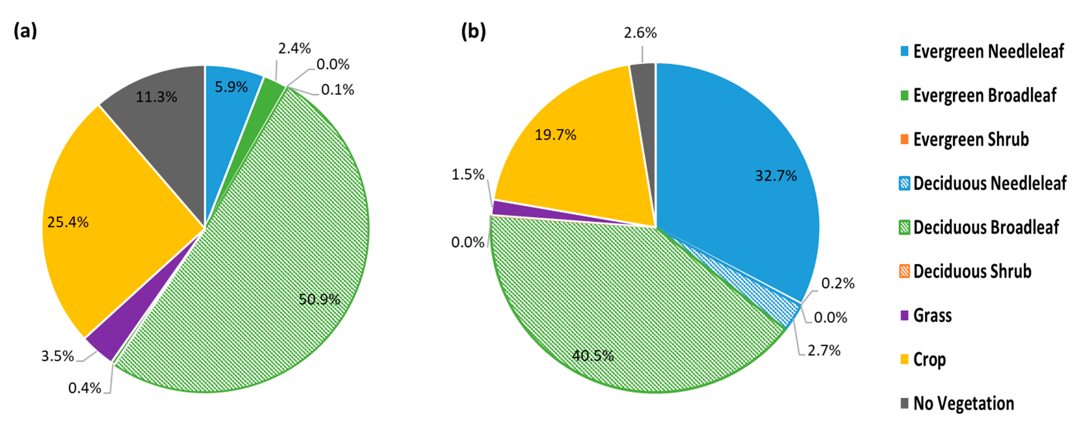
When using the same LAI, the use of Local PFT in cases 2 and 4 reduced isoprene emissions and increased monoterpenes emissions because the composition of the PFT had changed (
Figure 3). The portion of broadleaf trees decreased by 10% in the local PFT compared with the MODIS PFT, and the needleleaf trees increased by ~6 times. When we examined the Emission Factor (EF) for each PFT used in MEGANv2.1 [
8], isoprene EF decreases by 95% when changing from broadleaf to needleleaf trees; in monoterpenes, it increases by 50% for the same change. For this reason, when the Local PFT was used, isoprene emissions were reduced, while monoterpene emissions increased.
North Korea produced two emission cases (Case 1, Case 4) to changes in LAI (
Table 10). The lowest monthly isoprene emission estimates were for January (0.08 Gg/month in Case 1, and 0.18 Gg/month in Case 4), and the highest were in July (84.49 and 92.40 Gg/month, for cases 1 and 4, respectively). Total annual emission estimates for North Korea (Case 1 and Case 3) were 297.63 and 340.16 Gg/year, respectively, with Case 4 estimates 14% higher than those of Case 1 values.
For monoterpenes, January produced the smallest emission estimate in North Korea, with Case 1 yielding an estimate of 0.17 Gg/month, and Case 4 yielding 0.46 Gg/month. The largest monthly monoterpene emission estimates were in July, at 13.97 Gg/month and 16.26 Gg/month. Comparing Case 1 (59.43 Gg/year) to Case 4 (71.98 Gg/year). Case 4 values were 21% larger than Case 1 monoterpene emissions in North Korea. In most cases, North Korea showed the highest emissions in July (
Table 10). Unlike the rest of the Korean Peninsula, temperatures in North Korea were higher in July than in August, causing North Korea’s BVOC emissions to peak then, rather than in August.
Case 4 BVOC emission estimates were −8–101% higher than Case 1 estimates, depending on whether isoprene or monoterpene data were reviewed. However, when compared on a monthly basis, the differences were larger, with cold season estimates (January–March and November–December) more than twice as high; between May and August, differences were approximately 10%. In the cold season, local PFT and STARFM LAI estimates were relatively high compared with those of MODIS PFT and LAI, as described in
Section 3.1, reflecting a relative increase in Evergreen needle leaf forests in the local PFT.
4.2. Comparison with Inverse Estimates of BVOC Emissions
We used inverse emissions estimates from GlobEmission [
24] and observational data for 2015 to compare vegetation emissions from the Korean Peninsula. The isoprene emissions, provided by GlobEmission, were estimated using HCHO (formaldehyde) column concentrations, measured with an OMI (Ozone Monitoring Instrument) sensor. As of June 2020, GlobEmission provides monthly Global Biogenic Isoprene emissions for 2005–2014 (but not 2015). To compare isoprene emissions over the Korean Peninsula, the results of this study were compared with GlobEmission estimations for 2014. To make this comparison, we performed WRF modeling for 2014.
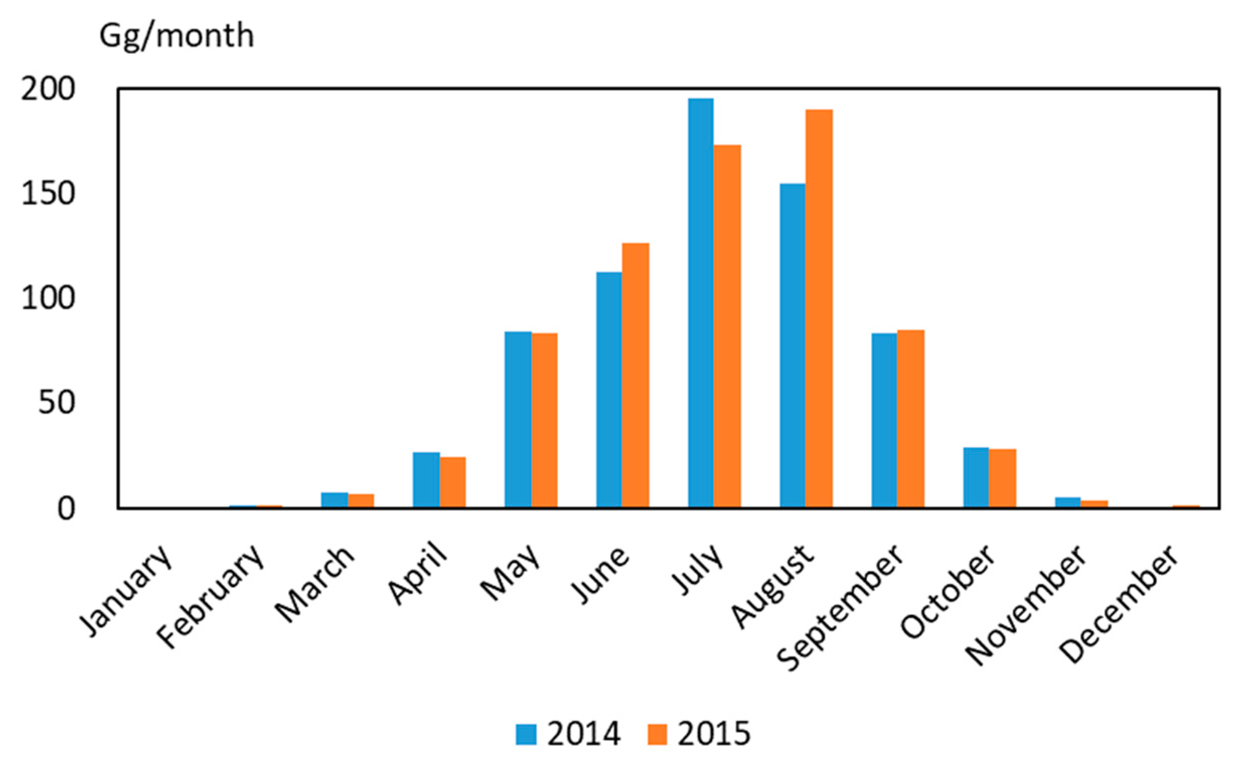
South Korea’s monthly isoprene emissions in 2014 and 2015 were compared using Case 4 (
Figure 8). Emissions in 2014 were 349.88 Gg/yr, 10% less than in 2015. Monthly variations showed greater variation than annual estimates. Usually, August has the highest temperature and humidity, which induces high vegetation emissions. In August 2014, isoprene emissions were 37% less than those of 2015 (
Figure 8). In 2014, two large typhoons affected South Korea, causing heavy rain in most parts of the country. Therefore, the average temperature was lower and the average precipitation was higher than the 30year average (year 1981~2010). Furthermore, more days of precipitation were recorded [
25]. Low daylight hours (74% of a normal year), were reflected in the lower isoprene emissions in 2014. As such, emissions in August 2014 and 2015 showed a marked difference; however,
Figure 9 shows that monthly emissions in 2014 were well estimated by the bottom-up modeling, since emissions showed a similar trend to GlobEmission.
Figure 9 shows 2014 bottom-up isoprene emissions estimated in this study and the inverse emission (GlobEmission) distributions. Using the bottom-up isoprene estimates for South Korea, Case 1 emission estimates for 2014 (373.85 Gg/year) were lower than those for 2015 (416.11 Gg/year); Case 4 emissions estimates showed the same trend (349.88 Gg/year for 2014 and 383.65 Gg/year for 2015). This reflects the two large typhoons in August 2014. The GlobEmission estimate for 2014 (260.71 Gg/year) was close to the Case 4 estimate (134%). For North Korea, the isoprene emission estimates for 2015 were lower than those of 2014. In the Case 1, annual emissions for 2015 were 297.63 Gg/year vs. 332.82 Gg/year for 2014. For Case 4, emissions were 340.16 Gg/ in 2015 and 351.83 Gg/year in 2014. For bottom-up to top-down inter-comparison, Case 1 values were closer (125%) than Case 4 values to the 2014 GlobEmission emission value (267.28 Gg/year).
Monthly isoprene emissions in South Korea (a) and North Korea (b) are inter-compared with GlobEmissions in
Figure 10. In general, bottom-up emissions showed similar monthly variations to GlobEmission emissions in 2014, with the highest emissions in July. In South Korea, the LAI and PFT for Case 1 and Case 4 were different, causing a difference in monthly emissions between these cases. Monthly emissions from May to July, when vegetation is active, showed a noticeable difference between cases, with estimations close to those of GlobEmissions in Case 4. Although emission amounts for Case 4 were larger than those of GlobEmission values (134%), the difference was smaller, considering that solar radiation shows a positive bias of ~15–20 (
Table 8). However, for North Korea, the difference between Case 1 and Case 4 was only observed for LAI, with no significant difference in emissions (7%) or patterns.
To compare emission estimation performances, bottom-up emissions for Case 1 and Case 4 were plotted with those of GlobEmission (
Figure 11). For Case 1, the slope was 1.59, and for Case 4, the slope was 1.09, with bottom-up emission results showing a tendency towards slight overestimation (i.e., positive bias). The correlation coefficient R showed high correlation (0.90). Even though both bottom-up emission cases overestimated isoprene emissions in June and July of 2014 for South Korea (
Table 11), the degree of agreement was much better for Case 4, which is consistent with the previous analysis.


 ,
, 


