1. Introduction
Among the main components of the global water cycle and the atmospheric circulation are evaporation, circulation wind, and precipitation [
1], and depicting their interplay is crucial to understand the dynamics of water vapor transport and the redistribution of energy. From a methodological perspective, most of the past studies that traced the pathways of humidity have used either numerical water vapor tracers, both in the Lagrangian approach (e.g., [
1,
2,
3,
4]) and the Eulerian approach (e.g., [
5,
6]), or physical water vapor tracers like the ones based on isotopes (e.g., [
2,
7]). Moreover, Drumond et al. [
8] used Lagrangian and Eulerian approaches to complement each other. Meanwhile, Esquivel-Hernández et al. [
2] and Windhorst et al. [
7] complemented their isotope-based studies with Lagrangian water vapor tracers.
Recently, however, the use of complex networks to identify causal flows, indicative of matter and energy flows, has gained much ground in climatology. This is a data-based approach that has been explored to characterize flows [
9] based on data only. This characterization is beneficial in two main ways [
10]: (1) it provides more information on known physical processes and mechanisms, and (2) it allows one to hypothesize on those that were previously unknown. Very importantly, if methods such as complex networks (based solely on data) are not used, some new hypotheses or mechanisms cannot be possibly found since traditional methods generally impose assumptions based on prior expert knowledge. Thereby, complex networks could be exploited to expand understanding of the humidity and wind relationship with rainfall. When using causal networks, regions or in situ observations are represented by nodes in a network structure. The association between nodes can, in turn, represent different types of physically meaningful connections (e.g., [
11,
12]), for example, between humidity and rainfall. Often a scalar-valued field of some physical variable is used as a proxy to characterize the underlying vector field causing the dynamical processes (e.g., [
10,
13]). Some studies have used this approach to study rainfall over South America (e.g., [
14,
15]). Nevertheless, to the best of our knowledge, studies based on causal networks (a kind of complex network) to gain insights on humidity sources and pathways, or to unveil homogeneous zones of humidity and wind influence, do not yet exist.
Here, a virtual control volume approach that resembles the Eulerian description of a flow field but purely data-based in design is proposed, which uses a causal network approach to infer causal flows that allow the tracing of pathways of influence between climatic variables. To assess the proposed methodology, the rainfall from Ecuador is taken as a case study. Thus, it is possible to verify if the proposed approach reproduces known patterns of the influence that humidity and wind at different altitudes have on rainfall and to evaluate the ability of this approach to infer new ones. Continuous areas of influence are discussed based on the use of satellite-based rainfall observations and humidity and wind data from a reanalysis climate model.
The objective of this paper is to propose a causal discovery-based virtual control volume approach to study climate. With the approach, the aim is to provide new information on known relationships between humidity/wind and rainfall, but more importantly, identify new hypotheses regarding the direction and altitude of the influence of those critical variables.
The paper starts with a brief review of climatic effects involved in the dynamics of rainfall in the region where the study area is located. This description presented in section two is essential for the following discussion of the results. Section three presents the proposed virtual control volume approach and a description of the causality test chosen to use in the setting of the approach. The settings that were used to evaluate the approach are described in section four. The results are described in section five, and some comments on the setting used are in section six. Finally, the conclusions of the paper are in section seven.
2. A Brief Background on the Climate of the Study Area
Oceans are the primary source of water vapor that, after advection, results in rainfall over the continents [
16]. About 10% of the 430,000 km
3 of water from oceans is evaporated annually and results in rainfall over land. Meanwhile, the local evapotranspiration recycles about 60% of this water [
17]. The mentioned advection is primarily carried out by the wind, though convective processes also play an important role. This highlights both the importance of oceans as the primary source of rainfall in the continents [
1] and the effects of local, regional, and global convective and advective processes that drive humidity pathways and the recirculation of water.
The processes mentioned above, which condition humidity pathways, have an intricated relationship. As an example, in South America, the influences of evaporation and advection from the Pacific Ocean [
18,
19], the Atlantic Ocean [
20,
21], the Amazon river basin [
22,
23], and local water recycling are some of the main factors that need to be accounted for to understand the spatiotemporal patterns in rainfall over land. Moreover, rainfall patterns depend on the meridional (tri cellular circulation) and zonal circulation of the atmosphere (e.g., the intertropical convergence zone (ITCZ), Walker circulation, trade winds), oceanic currents (e.g., El Niño), and the role of the Andes [
24] that govern the tropical climate conditions and, in turn, convection and precipitation patterns [
25].
On the other hand, regional and local low-level jet structures controlled by thermal gradients and topography like the western Colombian jet (CHOCO) [
26], the Caribbean [
27,
28], or the South America low-level jets (SALLJ) [
29], drive the rainfall distribution as the main advection factor for carrying humidity [
1,
3,
5,
6,
30].
The altitude at which these jets are stronger also reveals that the governing mechanisms should be analyzed at different altitudes since humidity content and wind show differences as they move away from sea level. Last but not least, quasi-periodic variations in ocean temperature across several temporal scales (e.g., El Niño Southern Oscillation (ENSO) and the Pacific decadal oscillation, (PDO) [
31]) produce anomalies in rainfall patterns (floods o droughts), in some cases with severe social consequences [
32,
33].
Ecuador is located in South America and was chosen as a remarkable case study because the Andes pass defines three climatic regions [
24], its extreme altitude gradients, and its location in the tropics. These conditions are responsible for an intricate spatiotemporal variability whose study has been considered as a complex task [
34]. An additional difficulty in studying the climate of Ecuador is the scarce monitoring network, which is typical for developing countries. This reality is even much more tangible nowadays in the Amazon region, where there are few stations without much data or with data of poor quality [
35]. To overcome this problem, efforts have been made using satellite-based observations to improve observational databases [
36,
37]. These databases constitute an excellent opportunity to experiment with data-based knowledge discovery techniques.
3. Methodology
3.1. Virtual Control Volume Approach to the Study of Causal Flows
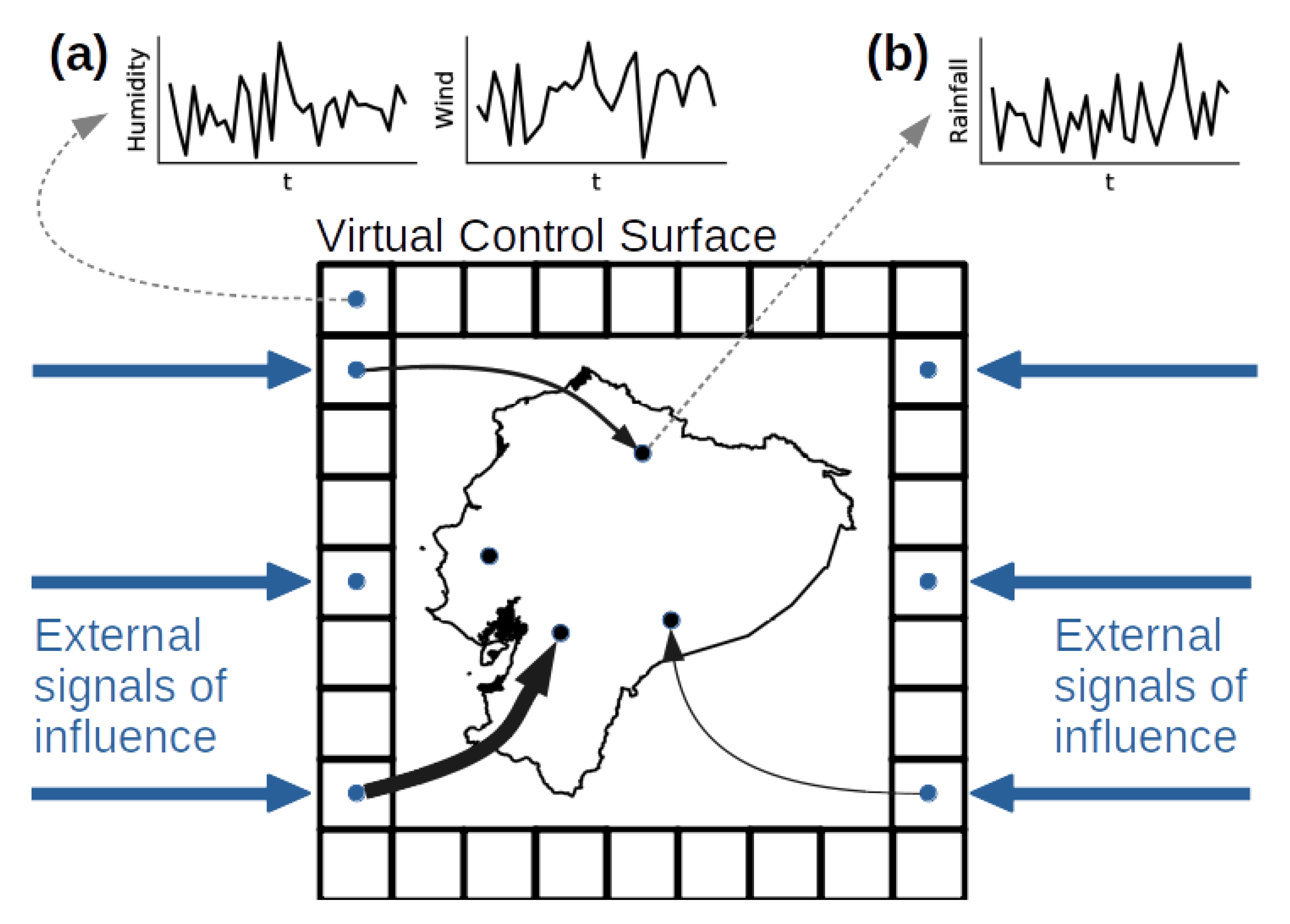
The approach uses a virtual monitoring region (the virtual control volume), reminiscent of a control volume through which a continuum flows, as well as the control surface that encloses it. In our proposed methodology, outlined in
Figure 1, a geographic region of interest (GRI) is enclosed by what has been named a virtual control surface where the flow of a physical quantity is analyzed (thick, larger, and straight arrows in
Figure 1). This flow is indirectly detected, employing a causal inference method providing the direction of influence and its intensity. More concretely, the virtual control surface is made up of a finite arrangement of points (or pixels for raster data), which contain information on some climatic variables (e.g., humidity as in
Figure 1a). In addition, in the enclosed geographic area, there is information on other climatic variables (e.g., rainfall as in Figre1b). Then, the influence from outside the virtual control volume is inferred using the information at the points on the corresponding virtual control surface as a proxy. In
Figure 1, this influence is schematized with the curved arrows between the virtual control surface and the GRI, and the intensity with the thickness of the arrows.
The continuous straight arrows in
Figure 1 schematize the possible input signals that are characterized by the information that is available on the virtual control surface. Different processes act on different time scales from days to decades [
38]. Thus, the time scale of the time series depicted in
Figure 1a,b should be chosen according to the time scale at the processes of interest probably act.
In the case of the analysis of the influence of humidity and wind outside the GRI on the rainfall inside that region, the control surface is operationally defined as a set of specific points storing time series of humidity and wind. Besides, in the GRI (the control volume), there are rainfall time series either in specific positions or symmetrically arranged positions, e.g., from satellite observations or climate models. Inference from external influence can be carried out using a causal inference method such as Granger causality, which has been used to infer matter and energy flows in the climate system [
11,
12], or any others such as those based on the theory of information [
39].
3.2. Granger Causality
In recent years, the use of causal inference methods to gain insights into the dynamics of complex systems like the climatic system has increased. A diversity of methods has been developed, and some of them deal with the particularities of the climate system [
39]. One of the underlying ideas in climate causality is the inference of flows, of which there are only scalar observations [
9]. Here the state of the art Granger causality method [
40] is used. The simple idea behind Granger causality (GC) is based on the ability of one variable to predict another, removing the influence of all other available variables considered in the system. For instance, the considered variables in this study are relative humidity, wind, and rainfall (
,
, and
respectively). It is considered that there is a causal connection from
to
(
) if the prediction of
given by a prediction model using all available past information of
,
, and
is better (often by a statistical test) than the prediction of
using the past information of
and
only. Although precedence in time is essential in causality, since a cause necessarily presides over an effect, sometimes subsampling a climatic variable or time-aggregation [
39] does not allow the inference of causal links because the wanted signal acts on a shorter time scale than the sampling frequency. For instance, monthly
data cannot be used for inferring causal connections toward monthly
. The reason is that water vapor resides in the atmosphere around 8–10 days [
41], that way,
signal acts instantly on a monthly time scale. Thus, connections on a daily or weekly scale, i.e., contemporary signals at a monthly scale, will not be reported. Due to the above, the inference method must take into account such particularities.
In his seminal work, Granger [
40] already discussed a general case of causality to take into account the case above. Granger defined instantaneous causality of
towards
(
) if the current value of
is better predicted including the present value of
(in addition to the past) than if it is not. Formally and borrowing the Granger [
40] terminology, given a stationary stochastic process
, the set of past values of the process will be represented by
. Then, the predictor of
using the set of values of the history of a different stochastic process
will be denoted by
, the predictive error series of
by
, and the variance of
by
. Then, standard Granger causality from
to
occurs if
, whereas instantaneous Granger causality
occurs if
. In the system with processes
and
influencing process
, instantaneous GC
occurs when
, and instantaneous GC
occurs when
.
For the predictor
, the ordinary least squares method is employed. More specifically, linear regression models are used, using a lag of one (i.e., the information of the past month and the present):
As a measure of how strong a causal connection is, the one defined by Hlinka et al. [
11] is utilized, which is computed as
where
reads as Granger’s instantaneous causal strength from
to
. The residual sum of squares (SSR) F-statistic was used to ensure that the improvement on the prediction of
using the present values of potential causal processes (
or
) has statistical significance, discarding connections with
p-value > 0.01.
In a system where the same variables are analyzed, the GC strength can be used to compare how coupled the processes are (i.e., between one causal connection found and another). This is why it is not necessarily plausible to make a comparison in terms of absolute values, e.g., with other studies that analyze other variables or different temporal or spatial scales since they could be unraveling different processes.
4. Assessment of the Proposed Approach
4.1. Study Area
Ecuador is located in the northwestern part of South America and is crossed by the equator as shown in
Figure 2a. The presence of the Andean mountain range defines three climatic regions [
24] whose limits are approximately at 1000 m a.s.l. both sides of the cordillera [
37,
42,
43,
44], i.e., the coast, Andean, and Amazon regions.
Figure 2a shows the common spatial delimitation of the Andean region as the zones above the 1000 m a.s.l., the delimitation of the coast, west of the Andes, and the Amazon region, east of the Andes. The rainfall climatology is different in each region (
Figure 2b), the Andes being the region with more heterogeneous spatiotemporal rainfall distribution due to the intricate western and eastern influences [
21]. A unimodal rainfall distribution characterizes the coastal region with a peak from February to April. The Andean region has a bimodal distribution with peaks in February–March–April and October–November–December. Meanwhile, the distribution in the Amazon, although the more copious precipitation in the whole country, does not show high variability [
35,
43,
45] but a peak exists from May to July. On the other hand, the spatial distribution of rainfall is heterogeneous in each region and with significant differences between the austral summer (DJF) and winter (JJA), as displayed in
Figure 3.
4.2. Data
The specific humidity (
) and the two horizontal components (i.e.,
and
) of wind data from 1981 to 2016 (36 y) from the NCEP/NCAR reanalysis [
46] were used. It has a monthly time step with a 2.5° × 2.5° spatial resolution. The wind and humidity variables were used at pressure levels of 1000, 850, and 600 hPa (i.e., approx. 100, 1500, and 4200 m a.s.l.) since humidity in the atmosphere is almost entirely contained in the lower troposphere, and because the Andean mountains in the study area reach on average 3500 m a.s.l. (around 680 hPa). Even though the wind is a vector field, in this study only the magnitude of the wind was considered (
), and from this point onward, it is what will be referred to as wind (
).
was selected because it has been used for computing variations in moisture and interpreting it as precipitation or evaporation (e.g., [
1,
34]), and
because it is considered one of the crucial factors to transport humidity. Moreover, Rossel and Cadier [
47] recommended using the upper atmosphere wind and air humidity for predicting rainfall in Ecuador, hinting their importance for understanding atmospheric mechanisms that explain continental rainfall.
Regarding the rainfall (
) data, the Climate Hazards Group Infrared Precipitation with Stations (CHIRPS; [
36]), with a spatial resolution of 0.05° × 0.05° and monthly time step, was used. CHIRPS is the result of merging ground-based observations and satellite products, and it has become a significant input where the complex topography of the study areas does not allow for in situ observations. CHIRPS data were pixel-wise validated against 45 ground stations for the whole country for the period 1981–2014, given the ground data availability. At each month, precipitation was recovered from ground stations and CHIRPS. Root mean square error (RMSE), correlation (Spearman), and percent bias (PBIAS) were calculated if at least there were ten ground stations for that month without missing values. As a result, a total of 378 months out from 408 were validated.
Each time series was first linearly detrended to minimize the influence of a possible climate change signal when computing causality. Since the only variables taken into account are , , and , eliminating interference of any other variable (as long as possible) helps to infer independent causal signals, in addition to the fact that there is no time series to represent the possible signal of climate change. After removing the linear trend, each time series was deseasonalized, calculating the standardized monthly anomalies (z-values) with respect to the whole time series. Thus, from this point onward , , and refer to anomalies.
4.3. Virtual Control Surface Setup
A squared boundary (the virtual control surface) around the limits of the study area (the virtual control volume) was set; this corresponds to the external pixels shown in
Figure 2a. As shown in
Figure 4, such square boundary limits are 7.5° S–2.5° N and 82.5° W–72.5° W, with spatial resolution 2.5°, which is determined by 16 pixels around Ecuador. Each of these pixels has been called Px
i,j, where i (j) corresponds to the row (column) of the square boundary. The inference of causal connections is carried out at the three pressure levels 1000, 850, and 600 hPa, from each pixel of the boundary (with data of
and
at each pixel) towards the rainfall in Ecuador (10,371 rainfall pixels).
With 16 pixels on the boundary and three levels, there are 16 × 3 = 48 observations for each time step for and 48 observations for . Further, the inference of the causal connections is performed for the austral summer (DJF) and winter (JJA). Only causal connections with statistical significance (p-value < 0.01) are taken into account. The results are shown as maps of GC strength that indicate how strong the causal connections from each pixel of the control surface to the rainfall are, i.e., indicating continuous areas where and present causal connection with and its strength, employing the GC strength fields (this for each pixel in the control surface, for each level, and each season; 192 maps in total).
5. Results and Discussion
Data validation was performed on a monthly scale from 1981 to 2014, whenever more than ten ground stations were available (i.e., without missing data). A total of 378 were validated, showing an RMSE median of 89.54 mm/month, a PBIAS% median of −0.28%, and a median correlation coefficient (Spearman) of 0.81. The results showed an acceptable validation for CHIRPS data countrywide.
5.1. Seasonality and General Variability Linked to the Altitude and Direction of the Connections
The influence of
and
on
presented substantial variability throughout the year and at different altitudes, with a clear distinction regarding the influence direction (from east or west). This confirms that the Andes act as a blocking element [
48], which defines rainfall patterns in the three regions.
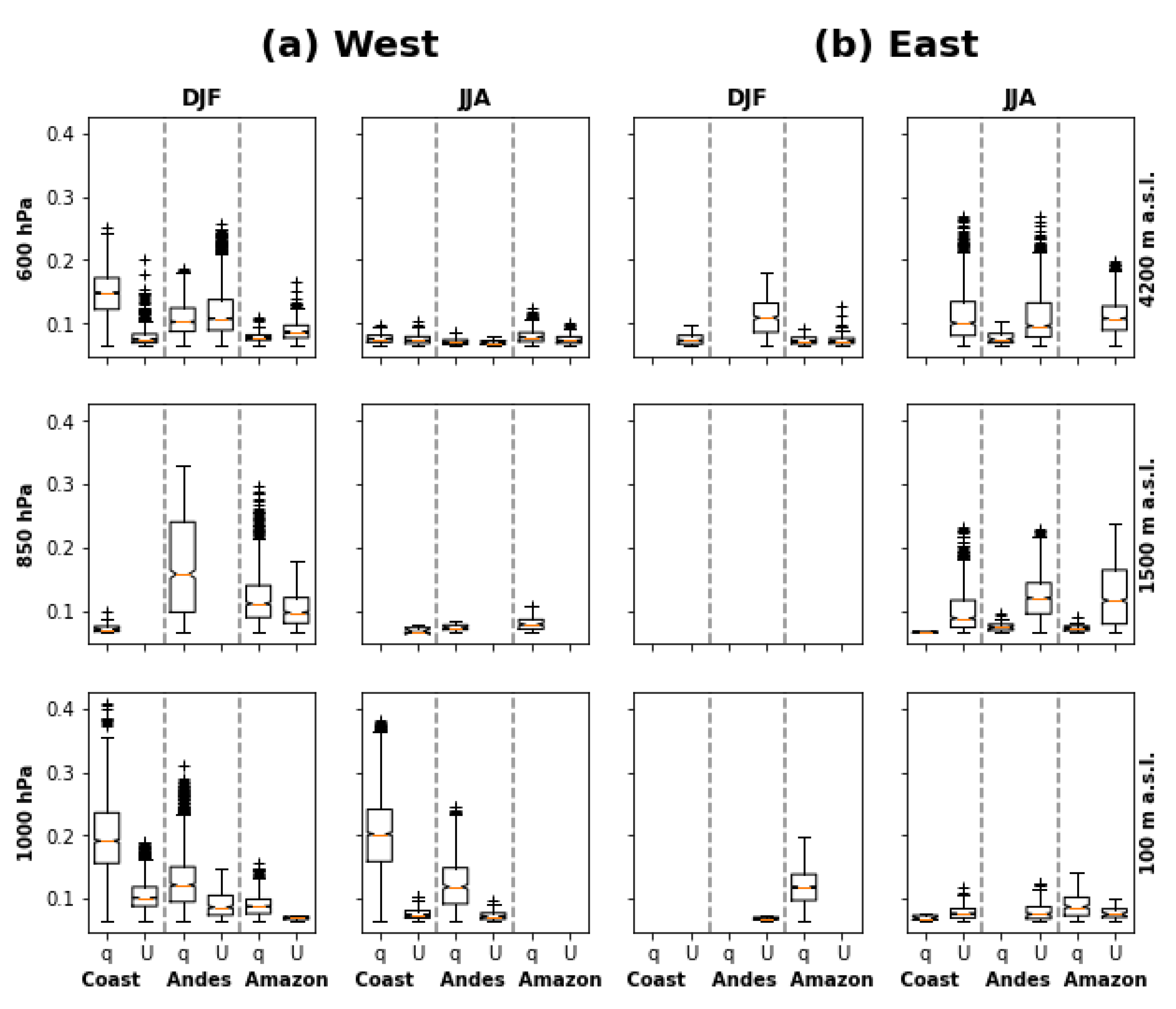
Figure 5a shows the causal connection strength (
and
toward
) from the west (striped Px
3,1 pixel in
Figure 4), near to the Guayaquil gulf. The GC strength is spread out in DJF and JJA (showed as columns) at different pressure levels (i.e., altitudes, shown as rows) for the three regions (coast–Andes–Amazon) separated by the dashed vertical lines. Similarly,
Figure 5b shows the GC strength from the east (striped Px
4,5 pixel in
Figure 4). Each boxplot shows the distribution of the GC strength between
and
(shown in the figure within each region) in pixels Px
3,1 (
Figure 5a) and Px
4,5 (
Figure 5b) toward
pixels in the three regions. The direction of the connections (beside the clear dependence of the altitude and season) allows for the division of the discussion horizontally, i.e., western and eastern influence; vertically, i.e., the lower troposphere, from 1000 to 850 hPa (approx. 100–1500 m a.s.l.) and the middle troposphere at 600 hPa (approx. 4200 m a.s.l.); and finally, in the austral summer (DJF) and winter (JJA).
From the west, there are the highest values of GC strength between
and
in the lowest troposphere during DJF and JJA (
Figure 5a, 1000 hPa). Independently of the season, the same pattern exists in the lowest troposphere, which shows the importance of
from the Pacific Ocean in the coastal region
during DJF and JJA. This strong
causal signal decreases at higher altitudes, appearing almost null at 850 hPa and with low values in the middle troposphere (
Figure 5a, 600 hPa). This behavior could be related to the high amount of humidity in the lower troposphere, where approximately 30% of the humidity in the atmosphere is present at 1000 hPa and 75% up to 850 hPa (calculated with NCEP/NCAR data in the study area). On the other hand, in general, during DJF and JJA,
shows higher values than
both in the lower and middle troposphere, but GC strength of
increases at higher altitude (with low content of humidity). Finally, in general, the GC strength (
and
over
) during DJF (coastal wet season) shows higher values than in JJA (coastal dry season). This change is according to the climatology of rainfall in Ecuador, especially in the coast (
Figure 2b and
Figure 3), where 80% of the annual rainfall occurs from December to May [
35]. Furthermore, this gives a clue about the strong influence of irregular variations of meteorological parameters of Pacific (western) origin in the rainfall, such as ENSO during DJF [
31].
The average altitude of the Ecuadorian Andes is around 3500 m a.s.l. and that is why a minimum signal of humidity reaches Andean zones promoting rainfall close to the division with coast. In regard to the known influence of the Pacific Ocean reaching the Andes region, the penetration of the signal is due to the sea surface temperature anomalies (SSTA) in the eastern Pacific [
49]. For example, the positive SSTA in the eastern Pacific is highly correlated with positive anomalies of humidity [
50] that result in the influence toward the western slopes of the Andes. Moreover, the signal of central Pacific anomalies is propagated throughout the mid-troposphere, affecting rainfall conditions in the Andes region [
51]. The arrival of the influence signal in the Amazon region is particularly noteworthy. Boxplots in
Figure 5a show the connection of
in the west with the Amazon region, beyond the Andes, which is related to the fact that under anomalous circulation, the signal goes further into the continent.
From the east, much more marked differences between DJF and JJA appear. Lower values of
and
exist concerning the west values in the lowest troposphere (
Figure 5b, 1000 hPa) that are practically null in DJF. Moreover, there are no connections from the east in DJF at 850 hPa. Contrary to the west, from the east,
presents higher values than
. This is more evident at 850 and 600 hPa (
Figure 5, first two rows from above). This could be related to the low-level jets, crucial in the transport of humidity from northeast South America and the tropical Atlantic, and probably the more important signal to define rainfall anomalies in the study area. Indeed, at 600 hPa the GC strength of
connections is practically the only from the east in JJA (
Figure 5b), which could be explained by the presence of the known mid-tropospheric easterly jet at approximately 600 hPa [
52] that connects the Atlantic and Pacific oceans across the northern Andes contributing to define an aerial river from April to August [
6], the season when this feature is more evident (see
Figure 5b at 600 hPa in JJA). Besides, from the east, during JJA, higher GC strength exists than during DJF, which in the west is the opposite.
In general, it is possible to notice differences in the GC strength between DJF and JJA, and between the connections from the east and the west toward the three climatic regions. It is important to note that from the west, humidity plays the leading role in the Ecuadorian rainfall anomalies (mainly in the coast), which change when analyzing the signals from the east, from where the wind is more important. This may be related to the bimodality of rainfall in the inter-Andean mountain range influenced by the Pacific during January–May [
53] and by the Amazon air in October and November [
54]. The results above evidence that the method proposed here is capable of identifying the seasonal patterns of the regions adequately. Furthermore, patterns in GC strength at the middle troposphere allow for the division of the analysis into two levels of altitude: lower troposphere (1000–850 hPa, approx. 100–1500 m a.s.l.) and middle troposphere (600 hPa, approx. 4200 m a.s.l.). Likewise, the analysis of the connections spatial patterns from this point onward is divided between the causal signals from the west and east.
5.2. Spatial Patterns of Connections and Strengths
Figure 6 and
Figure 7 show the direction of connections from
(left column: a, c, and e) and
(right column: b, d, and f) to
, and its GC strengths for DJF and JJA, respectively. Results for the 600, 850, and 1000 hPa levels are presented in each row from the highest altitude in the first row to the lowest altitude in the third row. For each pixel of the control surface at each level, there is a map indicating the GC strength of the connections between the pixel and the rainfall in the GRI (see
Figure 4). For example, the map entitled Px
1,5 in
Figure 6a indicates that there are connections between
in pixel Px
1,5 (
Figure 4) and
in the Amazon region, whose GC strength is indicated with the intensity of the color.
5.2.1. Western Humidity and Wind Connections to Rainfall
Humidity Connections to Rainfall
There was a strong causal connection of
in the eastern Pacific Ocean toward the coastal
at 1000 hPa, persistent in DJF and JJA. Additionally, this spatial pattern was also present at 600 hPa, but in DJF only (coastal wet season).
Figure 6a,e and
Figure 7e show how this robust signal spreads from zones close to the Gulf of Guayaquil, penetrating to higher altitudes corresponding to the highest elevations of the western slopes of the Andean mountain range. These results support the knowledge that rainfall anomalies on the coast are related to the conditions of the Pacific close to Ecuador and northern Peru (El Niño 1.2 region) [
47,
53]. Moreover, Rossel and Cadier [
47] demonstrated that SSTA from the previous month in the tropical Pacific close to the coast were the best predictors to forecast rainfall at the end of the wet season (April and May). Furthermore, Rossel et al. [
55] demonstrated that the increase in mean rainfall is superior to 40% due to ENSO events. According to our results, this known pattern was observed in both DJF and JJA (the wet and dry seasons of the coast, respectively).
The Granger causality test is not able to discriminate whether positive or negative humidity anomalies (
) are connected to positive or negative rainfall anomalies (
). However, anomalously high humidity has been previously reported as being related to positive rainfall anomalies in the coastal region [
50]. Moreover, having connections of
to
during the dry season of the coast (JJA) is admissible since this could be interpreted as if positive humidity anomalies exist, rainfall anomalies exist (the same with negative humidity anomalies).
Since the division between the coast and Andes used in this study is at 1000 m a.s.l., the connections of
could be patent toward zones of the Andean region (e.g., in
Figure 7), evidencing that the
regimen from the coast extends well above 1000 m a.s.l.. Concerning this specific result, Tobar and Wyseure [
45] clustered rainfall in four groups adding to the coast, Andean, and Amazon regions, an additional rainfall region between the Andes and coast called the Coast Orographic Sierra (COS). The COS region extends from the western foothills of the Andes until approximately the western highest Andean peaks. Indeed, the existence of the COS region is also the reason for the appearance of a certain connection between the pixel Px
3,1 (west) and the Andean region in
Figure 5a (e.g., at 850 hPa in DJF). Moreover, this similitude with the coastal influence might be responsible for the coastal-like seasonality present in western Andes [
56]. The COS region responds to the fact that the western slopes of the Andes trap humidity that, in part, results in orographic and convective rainfall (local heating) [
57]. Moreover, the anomalies of humidity in the eastern Pacific being linked to anomalies in the Pacific sea surface temperature (SST) causes atmospheric conditions that trigger convective processes linked to anomalies in rainfall [
58] that extend up to approximately 1800 m a.s.l. in the western Andes [
49], corresponding to approx. 1000–850 hPa. Above such altitude, the signal dissipates modulating the atmospheric circulation that inhibits convection in mountain zones [
48]. Our results regarding the penetration of
in the Andes confirms that rainfall in the western upper-elevation in the Andes is associated with high atmospheric humidity over the eastern Pacific, as mentioned by Hastenrath [
59], who states that in DJF, it is related to the southward position of the ITCZ.
Wind Connections to Rainfall
A minimum number of causal
connections from the west exists in the lower troposphere both in DJF and JJA (
Figure 6 and
Figure 7). The GC strength of those connections is lower than the
ones, which means that
provides less information to explain
than
. During DJF, the connections of
at 1000 hPa (
Figure 6) from the west toward
have a spatial pattern similar to
toward the coast, but with much lower GC strength. This responds to the dominant forcing of
due to the effect of SSTA in the eastern Pacific. In DJF, western winds transport humidity from the Pacific Ocean and generate rainfall in the coast, even penetrating southwestern Andes [
53], as shown in
Figure 6. In these southern Andean zones, rainfall depends mainly on wind magnitude and direction, which are modified by topographic conditions forming barriers and humidity transport pathways [
57]. In our study, even though only wind magnitude was taken into account, the results confirm the known incidences of the wind magnitude presented by Fries et al. [
57].
While the influence of
comes through the lower troposphere, at higher altitudes, the results give new insights on
playing a crucial role. Western
presents connections toward the Andean region at higher altitudes (600 hPa) in DJF (
Figure 6b).
Figure 6b shows the clear delimitation of the influence of wind over the precipitation anomalies in the Andean region. Since the Andes rainfall is in part related to the conditions of the central Pacific (El Niño 3.4 region) [
60], a possible mechanism acting here responds to the signal of the central Pacific anomalies propagated throughout the mid-troposphere, affecting rainfall conditions in the Andean region [
51].
Interestingly, during JJA, the northwestern
pixels Px
2,1, Px
1,1, and Px
1,2 show a connection to the eastern slopes of the northern Ecuadorian Andes at 1000 hPa (
Figure 7). This newly found pattern constitutes a new hypothesis that could be related to the influence of the CHOCO low-level jet that has its peak during JJA [
26]. The signal comes from the coasts of South America. After propitiating rainfall in Colombia [
6], part of the humidity probably goes to the eastern Ecuadorian Andes, principally conveyed by winds in JJA, while in DJF (
Figure 6), this is achieved by local factors (without the primary influence of wind) (see
influence in
Figure 6e,c, northwestern pixels). Bendix and Lauer [
61] already argued that the rainfall in the February–April period is related to atmospheric processes of the eastern Pacific region and winds from the Panama Gulf. The mentioned Panama Gulf winds are probably related to the Caribbean low-level jet. A possible mechanism working here is the influence of the low-level jet that brings humidity from the south of the eastern Pacific towards the CHOCO that, after colliding with the influence of the Caribbean low-level jet (LLJ), moves its influence towards the south in the direction of the Andes [
6,
7,
61]. Windhorst et al. [
7] found a trajectory following the raised hypothesis using the hybrid single-particle Lagrangian integrated trajectory (HYSPLIT) model, but it does not constitute conclusive proof of the hypothesis. Studying this new hypothesis is a crucial topic in gaining insights into the causes of precipitation in the Andes–Amazon northern division region and probably the coast–Andes northern division region too. Moreover, it shows that using our approach to study these connections can give new insight into patterns like those found.
5.2.2. Eastern Humidity and Wind Connections to Rainfall
Contrary to the pixels of the Pacific Ocean (western influence), in general, pixels in the east present differences from each other. For example, refer to
Figure 6e where pixels Px
1,5 and Px
4,5 present different patterns of the GC causality strength fields, contrary to the pixels Px
1,1, Px
2,1, …, Px
5,1 in the west. The heterogeneous influence from the east displays the complex influence from the southern and northern tropical Atlantic, and the Amazon basin. Some connections from eastern pixels reach the coastal region (this is seen in
Figure 5b too), but with a view in the spatial distribution of these zones (e.g., see
Figure 7c,d), the points should be considered spurious.
Humidity Connections to Rainfall
While SST over the central and eastern tropical Pacific influences the coast and the western Andes,
over the eastern Andes and Amazon region is connected with SSTA in the tropical Atlantic Ocean [
45,
51,
60,
62]. However, a particular distinction between the influence from the northeast and southeast must be made. In DJF,
northeastern pixels at 600 hPa are connected to
in zones in the Amazon, which could respond to the influence of the northern tropical Atlantic (
Figure 6a). Meanwhile, the
southeastern pixels at 1000 hPa (
Figure 6e) are connected to the same zones in the Amazon. These new findings suggest that the altitude of the influence of the southern tropical Atlantic is different from that of the northern tropical Atlantic.
Figure 6 shows that the most important feature in DJF is the causal connection of
toward
in the Amazon region from the east but with a differentiated influence according to the altitude. While in the lower troposphere, the connections toward
in the Amazon comes from the southeast (
Figure 6e), at higher altitudes (600 hPa), the influence comes from the northeast (
Figure 6a). Regarding this feature in DJF, Drumond et al. [
8] showed the influence of the tropical Atlantic towards the Amazon river basin (the Ecuadorian Amazon is located within it), and a division between the influence of the northern and southern tropical Atlantic is evident [
1]. According to our new findings, such influence may have its pathways at different altitudes. Thus, the Ecuadorian Amazon receives the
influence as high as approximately 850 hPa (approx. 1500 m a.s.l.) from the southern tropical Atlantic and the influence at altitudes higher than 850 hPa from the northern tropical Atlantic (
Figure 8a). This is consistent with the known influence of the South American low-level jet that is the primary conveyor of humidity and factors for producing rainfall in South America. Meanwhile, higher winds act from the northern tropical Atlantic.
From January to May, most of the humidity comes from the North Atlantic [
8]. According to the work of Durán-Quesada et al. [
1], using part of the Amazon region of Colombia as the bounded area to the analysis employing the FLEXible PARTicle dispersion model (FLEXPART), a similar pattern was found, the North Atlantic being the primary source of humidity to the Amazon region of Colombia (the bounded area has its limit with the study area).
Figure 6a gives evidence of the source of moisture during the austral summer, coming from the Atlantic and penetrating to eastern flanks of the Andes in the east–west direction. Consistent with this result, Esquivel-Hernández et al. [
2] analyzed air mass back trajectories for a high altitude station in the eastern Andes and showed the North Atlantic Ocean and the Caribbean Sea as a source of moisture during El Niño conditions.
Wind Connections to Rainfall
While in DJF
connections suggest a northeastern influence at high altitudes (600 hPa) and a southeastern influence at lower altitudes (1000 hPa) of humidity anomalies, in JJA, the differentiated pattern of influence according to the altitude is the same, but with
being the primary factor (
Figure 8b). These GC strength fields of
from the northeast pixels at 600 hPa (
Figure 7b) show the connection of
with
in the Amazon and in the zones between the Andean and the Amazon region following the broad river valleys, Paute, and Pastaza that may be related to the advection of humidity generated by
, as found by Tobar and Wyseure [
45]. The wind influence in this season is explained by the peak of easterly winds during JJA (
Figure 9) that causes the wet season in the western Amazon (evidenced in
Figure 3b) [
21,
45,
56] and is associated with the SALLJ [
34,
63]. In the same way, strong humidity transportation from the Amazon and orographic uplift is the cause of rainfall in the eastern Andes foothills (
Figure 3b) [
34]. The strong easterly winds in JJA may enhance rainfall in the upper zones of the Andes. However, because of the lower atmospheric humidity and large-scale subsidence, such rainfall remains reduced in the upper-elevation Andes [
34]. Thus, humidity from the Atlantic and Amazon ends in rainfall in the central-eastern Andean foothills and western Amazon, as shown in
Figure 7b.
Moreover, the results corroborate the results of the vertically integrated water vapor flux shown by Segura et al. [
34] (their
Figure 1). The influence of the tropical Atlantic is mainly due to the SALLJ and easterly trade winds. The proportion of trade winds from June to September is close to 100% [
65]. This is the reason why a strong influence of eastern winds is observed over the eastern slopes, defining areas of high rainfall rates in the Andean region during JJA (
Figure 3b). Drumond et al. [
8] show a clear difference of moisture sources between JJA and DJF seasons, analyzing particles bound for the Amazon basin, whose area includes the Amazon region of Ecuador. During JJA, most of the moisture resulting in sinks over the Amazon region of Ecuador seems to come from the South Atlantic. Meanwhile, Windhorst et al. [
7] found enriched heavy isotopes in a southeastern Andean observatory, revealing a contribution of the Amazon basin by recycled moisture in the air masses in this zone.
6. Comments on the Proposed Setting
Concerning the resolution of the data in the virtual control surface, this should be chosen to synthesize information coming from the exterior. In the use case, the resolution of NCEP/NCAR is sufficient to synthesize the entrance of regional signals mainly from the north, south, east, west, and some intermediate directions. The impact of the scale on the results of the causality tests depends on how “wide” the input signal is. If the signal goes through several pixels of the virtual control surface, a pairwise causality test (between
/
toward
) will probably show redundant results. As an example, in the pixels corresponding to the longitude 82.5° W (Px
1,1, Px
2,1, …, Px
5,1) of
Figure 6e, the results are similar, which shows that the influence from the Pacific Ocean is considerably wide since its effects can be observed in all the pixels on the left of the virtual control surface. Thus, a higher resolution would probably have shown redundant results in neighboring pixels.
Regarding the spatial resolution of the rainfall, humidity, and wind products, even if they have different spatial resolutions, in the virtual control volume approach, the pixel time series are used for the analysis (temporal analysis pixel-wise). Thus, the original spatial resolution of each product was kept, and not spatial resampling method was used.
Regarding voids or zero values in the time series, since the application of the virtual control volume approach is based on remote sensing and reanalysis data, all the time series have continuous data. If the data source were, for instance, in situ weather stations, infilling methods might be useful to complete the time series. Additionally, since the application was made in a tropical area, we did not get any monthly zero precipitation (importantly, anomalies were always used).
Regarding the use of wind magnitude, there are no mathematical limitations in using the virtual control volume approach as long as the variables can be represented by time series. Therefore, it is possible to take into account all the components of the wind in a much more exhaustive analysis.
GC has been shown to find directed relationships between climatic variables. However, one of the disadvantages is that it does not directly identify whether the dependency is positive or negative. For example, if there is a connection between wind and rain, it cannot be ensured that higher wind values imply higher precipitation values or vice versa. Other causality tests could be used with the virtual control volume approach to deal with this issue.
GC is quite robust concerning high correlation over time [
66]. However, the use of GC in the proposed approach does not allow for the determination of the causal relationships from each of the pixels on the control surface independently. This is due to the high spatial correlation of the data. For example, a possible reason to have a signal from the west to the northern pixels in
Figure 6c could be produced by spatial correlations. Thus, the signal from the west (over the eastern Pacific) is correlated with the signal of the north of Ecuador (by any other mechanism). As a result, the signal is present in the eastern slopes of the Andes. Importantly, this signal could be highly correlated because of the influence of the CHOCO low-level jet or the temporal resolution used in the study, this signal being faster than the temporal resolution of the samples (monthly); this is known as a subsampling problem [
39]. Since GC does not take into account the direction of the wind in the inference but the magnitude only, this magnitude of wind in the eastern pacific allows us to obtain information on the precipitation of the northeastern Andes. A possible solution using GC is to explore a configuration that uses the information of an eastern and northern pixel for outperforming prediction over using only a northern pixel. Thus, the method rules out the spatial correlation in the same way as when a high autocorrelation in time is present with a unique source of influence.
In the virtual control volume approach, the causal inference method is essential. The use of causal inference allows us to observe asymmetric relationships. More importantly, unlike correlations, causal connections evidence directed relationships with a physical sense [
13], for example, transfer of energy and matter [
11,
12]. However, the use of GC does not allow the differentiation of anomalies (positive or negative) of wind/humidity that are related to anomalies (positive or negative) of the rainfall from those that would require a complementary analysis using the obtained causal relationships.
Among the other causal inference methods that can be used to test causality in the proposed approach are those based on information theory. This is a powerful framework to analyze asymmetric linear and nonlinear associations between information in the virtual control surface and the virtual control volume. An analog to Granger causality from the perspective of information theory is transfer entropy [
67], which allows for the analysis of the directed transfer of information between two variables, improving the proposed approach, including possible nonlinear associations. Another method based on the conditional independence framework is PCMCI [
68,
69]. Among the advantages of PCMCI is the quantification of the causal strength in a more physically interpretable way. These are just two examples of sophisticated methods alternative to Granger causality. A detailed list of methods can be found in [
39].
7. Conclusions
Causality-based methods are gaining much ground in the area of geosciences [
9,
10,
39]. In this study, we proposed an approach exploiting the state of the art Granger causality method for inferring causal relationships from humidity and wind anomalies over rainfall anomalies in a tropical study area whose spatiotemporal features are characterized by the complex influence of the Andean mountain range, the ITCZ, the Amazon river basin, and the tropical Pacific and Atlantic oceans, among several other factors. The inferred causal connections worked as a proxy to characterize physical connections among the variables. For this, the concepts of virtual control volume and surface were introduced. They are based on the concepts of control volume and control surface from continuum mechanics. Their “virtual” versions are defined within the framework of causal discovery, a data-based approach. The idea is to identify patterns of influence: some already known and, more interestingly, some that are currently unknown. The unknown patterns are regarded as new hypotheses that have to be contrasted. Thus, it is possible to estimate the independent contributions of the critical variables (humidity and wind) and their influence on rainfall.
In geosciences, causality has been used in different tasks, but, in general, two main aims are pursued. First, it seeks to gain insights on known features of the climate system, and second, to discover new hypotheses about underlying mechanisms or dynamics. With these ideas in mind, the proposed approach was evaluated. The well-known influence from the Pacific and Atlantic Oceans in the study area was confirmed. Our approach was able to provide further information about the influence of humidity and wind at different altitudes and delineate areas of influence geographically. Moreover, it was possible to propose new plausible hypotheses.
More in detail, the results show the ability of the virtual control volume approach to infer known physical processes related to the rainfall in the three climatic regions of the study area and to gain insights into some physical processes in the rainfall dynamics. Moreover, the fine grid of rainfall information allowed us to define continuous spatial patterns of influence of humidity and wind that change throughout seasons. Thus, the eastern Pacific Ocean has a definite influence on the rainfall in the coast region and the western Andes. Meanwhile, the eastern Andes and the Amazon regions are influenced by the eastern winds and humidity, whose sources are the Amazon river basin and the southern and northern tropical Atlantic at different altitudes.
Although many known associations could be confirmed, the complex mechanisms acting on the inter Andean valleys rainfall does not allow the method to find the relationships that were expected. Two reasons could be responsible for this: 1) the time scale used in the study does not allow the method to infer connections that are acting in a shorter time scale; or 2) more localized phenomena act in rainfall anomalies in the Andean region that are related to the complex interplay between western and eastern influences.
Furthermore, it was possible to enunciate new plausible hypotheses such as the influence of humidity on rainfall in the northern part of the boundary between the Andes and the Amazon, as well as the origin (the Amazon or the tropical Atlantic) and the altitude at which surrounding humidity and wind influence rainfall within the control volume. This highlights the power of causal network methods to exploit a large amount of scalar data and identify pathways of influence between climatic variables.
Additionally, the virtual control volume approach using gridded data allowed us to study causal flows at different altitudes and identify that humidity causing rainfall in the coast and the western Andes has its pathways at the lower troposphere (approx. < 1500 m a.s.l.). Meanwhile, wind plays a crucial role in the Andean rainfall, whose pathways are in the mid-troposphere. Concerning the eastern influence, there exist patterns that are more complex than in the west. In the Amazon wet season (JJA), the influence of wind changes its direction according to the altitudes. Thus, a southeastern influence has its pathways at the lower troposphere, while northeastern influence is defined in the middle troposphere. The same patterns were found in DJF but for the humidity variable.
In any case, a northern influence was found towards the northern limits between the coast and Andean regions and Andean and Amazon regions. We hypothesize that this can be related to the anomalous behavior of the CHOCO and the Caribbean LLJ, located to the north of our study area. However, this hypothesis must be studied in more detail. Moreover, and from the causal inference method used in the proposed approach, although GC works very well, excluding the presence of highly correlated signals over time, it is evident that its use can be improved to avoid the effects of high spatial correlation. The proposal to use a different configuration to suppress the high spatial correlation between the pixels on the control surface to find a single source of influence is an idea that would be worth exploring.
The approach presented is a combination of climate science and the Granger causality test. This work contributes to the efforts directed to bridge the knowledge gaps regarding the climate system through causality discovery methods that take advantage of the massive amounts of data that are available today.
Author Contributions
Conceptualization, L.C. and A.V.-P.; methodology, A.V.-P.; software, A.V.-P.; validation, M.C. and L.C.; formal analysis, A.V.-P.; investigation, A.V.-P.; resources, D.B., L.C., and E.S.; data curation, A.V.-P.; writing—original draft preparation, A.V.-P.; writing—review and editing, all authors; visualization, A.V.-P.; supervision, E.S., D.B., and L.C.; project administration, D.B. and E.S.; funding acquisition, D.B. All authors have read and agreed to the published version of the manuscript.
Funding
This research was funded by RED CEDIA through the CEPRA XII-2018 project “Representación espacial de las teleconexiones climáticas en la precipitación del Ecuador”.
Acknowledgments
This manuscript is an outcome of the Doctoral Program in Water Resources, offered by Universidad de Cuenca, Escuela Politécnica Nacional, and Universidad Técnica Particular de Loja. The authors thank the reviewers for the valuable comments that allowed to improve the manuscript.
Conflicts of Interest
The authors declare no conflict of interest.
References
- Durán-Quesada, A.M.; Reboita, M.; Gimeno, L. Precipitation in tropical America and the associated sources of moisture: A short review. Hydrol. Sci. J. 2012, 57, 612–624. [Google Scholar] [CrossRef]
- Esquivel-Hernández, G.; Mosquera, G.M.; Sánchez-Murillo, R.; Quesada-Román, A.; Birkel, C.; Crespo, P.; Célleri, R.; Windhorst, D.; Breuer, L.; Boll, J. Moisture transport and seasonal variations in the stable isotopic composition of rainfall in Central American and Andean Páramo during El Niño conditions (2015–2016). Hydrol. Process. 2019, 33, 1802–1817. [Google Scholar] [CrossRef]
- Sakamoto, M.S.; Ambrizzi, T.; Poveda, G. Moisture Sources and Life Cycle of Convective Systems over Western Colombia. Adv. Meteorol. 2011, 2011, 890759. [Google Scholar] [CrossRef]
- Trachte, K. Atmospheric Moisture Pathways to the Highlands of the Tropical Andes: Analyzing the Effects of Spectral Nudging on Different Driving Fields for Regional Climate Modeling. Atmosphere 2018, 9, 456. [Google Scholar] [CrossRef] [Green Version]
- Arraut, J.M.; Satyamurty, P. Precipitation and Water Vapor Transport in the Southern Hemisphere with Emphasis on the South American Region. J. Appl. Meteorol. Clim. 2009, 48, 1902–1912. [Google Scholar] [CrossRef]
- Poveda, G.; Jaramillo, L.; Vallejo, L.F. Seasonal precipitation patterns along pathways of South American low-level jets and aerial rivers. Water Resour. Res. 2014, 50, 98–118. [Google Scholar] [CrossRef]
- Windhorst, D.; Waltz, T.; Timbe, E.; Frede, H.-G.; Breuer, L. Impact of elevation and weather patterns on the isotopic composition of precipitation in a tropical montane rainforest. Hydrol. Earth Syst. Sci. 2013, 17, 409–419. [Google Scholar] [CrossRef] [Green Version]
- Drumond, A.; Marengo, J.; Ambrizzi, T.; Nieto, R.; Moreira, L.; Gimeno, L. The role of the Amazon Basin moisture in the atmospheric branch of the hydrological cycle: A Lagrangian analysis. Hydrol. Earth Syst. Sci. 2014, 18, 2577–2598. [Google Scholar] [CrossRef] [Green Version]
- Donner, R.V.; Lindner, M.; Tupikina, L.; Molkenthin, N. Characterizing Flows by Complex Network Methods. In A Mathematical Modeling Approach from Nonlinear Dynamics to Complex Systems; Macau, E.E.N., Ed.; Springer International Publishing: Cham, Switzerland, 2019; Volume 22, pp. 197–226. ISBN 978-3-319-78511-0. [Google Scholar]
- Ebert-Uphoff, I.; Deng, Y. Causal Discovery in the Geosciences—Using Synthetic Data to Learn How to Interpret Results. Comput. Geosci. 2017, 99, 50–60. [Google Scholar] [CrossRef] [Green Version]
- Hlinka, J.; Jajcay, N.; Hartman, D.; Paluš, M. Smooth information flow in temperature climate network reflects mass transport. Chaos Interdiscip. J. Nonlinear Sci. 2017, 27, 035811. [Google Scholar] [CrossRef] [Green Version]
- Vázquez-Patiño, A.; Campozano, L.; Mendoza, D.; Samaniego, E. A causal flow approach for the evaluation of global climate models. Int. J. Clim. 2020, 40, 4497–4517. [Google Scholar] [CrossRef]
- Molkenthin, N.; Rehfeld, K.; Marwan, N.; Kurths, J. Networks from Flows-From Dynamics to Topology. Sci. Rep. 2014, 4, 4119–4123. [Google Scholar] [CrossRef] [PubMed] [Green Version]
- Ciemer, C.; Boers, N.; Barbosa, H.M.J.; Kurths, J.; Rammig, A. Temporal evolution of the spatial covariability of rainfall in South America. Clim. Dyn. 2017, 51, 371–382. [Google Scholar] [CrossRef]
- Guo, H.; Ramos, A.M.T.; Macau, E.E.N.; Zou, Y.; Guan, S. Constructing regional climate networks in the Amazonia during recent drought events. PLoS ONE 2017, 12, e0186145. [Google Scholar] [CrossRef]
- Gimeno, L.; Drumond, A.; Nieto, R.; Trigo, R.M.; Stohl, A. On the origin of continental precipitation. Geophys. Res. Lett. 2010, 37. [Google Scholar] [CrossRef]
- Gimeno, L.; Nieto, R.; Drumond, A.; Durán-Quesada, A.M.; Stohl, A.; Sodemann, H.; Trigo, R.M. A close look at oceanic sources of continental precipitation. Eos Trans. Am. Geophys. Union 2011, 92, 193–194. [Google Scholar] [CrossRef] [Green Version]
- Gallego, D.; García-Herrera, R.; Gómez-Delgado, F.D.P.; Ordoñez-Perez, P.; Ribera, P. Tracking the moisture transport from the Pacific towards Central and northern South America since the late 19th century. Earth Syst. Dyn. 2019, 10, 319–331. [Google Scholar] [CrossRef] [Green Version]
- Hoyos, I.; Cañón-Barriga, J.; Arenas-Suárez, T.; Dominguez, F.; Rodríguez, B.A. Variability of regional atmospheric moisture over Northern South America: Patterns and underlying phenomena. Clim. Dyn. 2019, 52, 893–911. [Google Scholar] [CrossRef]
- Arias, P.A.; Martínez, J.A.; Vieira, S.C. Moisture sources to the 2010–2012 anomalous wet season in northern South America. Clim. Dyn. 2015, 45, 2861–2884. [Google Scholar] [CrossRef]
- Campozano, L.; Célleri, R.; Trachte, K.; Bendix, J.; Samaniego, E. Rainfall and Cloud Dynamics in the Andes: A Southern Ecuador Case Study. Adv. Meteorol. 2016, 2016, 3192765. [Google Scholar] [CrossRef] [Green Version]
- Boers, N.; Marwan, N.; Barbosa, H.M.J.; Kurths, J. A deforestation-induced tipping point for the South American monsoon system. Sci. Rep. 2017, 7, 41489. [Google Scholar] [CrossRef] [PubMed]
- Builes-Jaramillo, A.; Marwan, N.; Poveda, G.; Kurths, J. Nonlinear interactions between the Amazon River basin and the Tropical North Atlantic at interannual timescales. Clim. Dyn. 2018, 50, 2951–2969. [Google Scholar] [CrossRef]
- Pourrut, P. (Ed.) El Agua en el Ecuador: Clima, Precipitaciones, Escorrentía; Estudios de Geografía; ORSTOM, Colegio de Geógrafos del Ecuador and Corporación Editora Nacional: Quito, Ecuador, 1995; Volume 7. [Google Scholar]
- Insel, N.; Poulsen, C.J.; Ehlers, T.A. Influence of the Andes Mountains on South American moisture transport, convection, and precipitation. Clim. Dyn. 2010, 35, 1477–1492. [Google Scholar] [CrossRef]
- Poveda, G.; Mesa, O.J. On the existence of Lloró (the rainiest locality on Earth): Enhanced ocean-land-atmosphere interaction by a low-level jet. Geophys. Res. Lett. 2000, 27, 1675–1678. [Google Scholar] [CrossRef] [Green Version]
- Amador, J.A. A Climatic Feature of the Tropical Americas: The Trade Wind Easterly Jet. Tópicos Meteorológicos Y Oceanográficos 1998, 5, 91–102. [Google Scholar]
- Whyte, F.S.; Taylor, M.A.; Stephenson, T.S.; Campbell, J.D. Features of the Caribbean low level jet. Int. J. Clim. 2007, 28, 119–128. [Google Scholar] [CrossRef]
- Marengo, J.A.; Soares, W.R.; Saulo, C.; Nicolini, M. Climatology of the Low-Level Jet East of the Andes as Derived from the NCEP–NCAR Reanalyses: Characteristics and Temporal Variability. J. Clim. 2004, 17, 2261–2280. [Google Scholar] [CrossRef] [Green Version]
- Amador, J.A. The Intra-Americas Sea Low-level Jet. Ann. N. Y. Acad. Sci. 2008, 1146, 153–188. [Google Scholar] [CrossRef] [Green Version]
- Sanabria, J.; Carrillo, C.M.; Labat, D. Unprecedented Rainfall and Moisture Patterns during El Niño 2016 in the Eastern Pacific and Tropical Andes: Northern Perú and Ecuador. Atmosphere 2019, 10, 768. [Google Scholar] [CrossRef] [Green Version]
- CEPAL. Natural Disasters of 1982-1983 in Bolivia, Ecuador and Perú; Naciones Unidas-Consejo Económico y Social-Comisión Económica para América Latina: Santiago, Chile, 1983. [Google Scholar]
- Terneus, A.; Gioda, A. In search of colonial El Niño events and a brief history of meteorology in Ecuador. Adv. Geosci. 2006, 6, 181–187. [Google Scholar] [CrossRef] [Green Version]
- Segura, H.; Junquas, C.; Espinoza, J.C.; Vuille, M.; Jauregui, Y.R.; Rabatel, A.; Condom, T.; Lebel, T. New insights into the rainfall variability in the tropical Andes on seasonal and interannual time scales. Clim. Dyn. 2019, 53, 405–426. [Google Scholar] [CrossRef]
- Morán-Tejeda, E.; Bazo, J.; López-Moreno, J.I.; Aguilar, E.; Azorín-Molina, C.; Sanchez-Lorenzo, A.; Martínez, R.; Nieto, J.J.; Mejía, R.; Martín-Hernández, N.; et al. Climate trends and variability in Ecuador (1966-2011). Int. J. Climatol. 2016, 36, 3839–3855. [Google Scholar] [CrossRef] [Green Version]
- Funk, C.; Peterson, P.; Landsfeld, M.; Pedreros, D.; Verdin, J.; Shukla, S.; Husak, G.; Rowland, J.; Harrison, L.; Hoell, A.; et al. The climate hazards infrared precipitation with stations—A new environmental record for monitoring extremes. Sci. Data 2015, 2, 150066. [Google Scholar] [CrossRef] [Green Version]
- Ulloa, J.; Ballari, D.; Campozano, L.; Samaniego, E. Two-Step Downscaling of Trmm 3b43 V7 Precipitation in Contrasting Climatic Regions With Sparse Monitoring: The Case of Ecuador in Tropical South America. Remote Sens. 2017, 9, 758. [Google Scholar] [CrossRef] [Green Version]
- Williams, P.D.; Alexander, M.J.; Barnes, E.A.; Butler, A.H.; Davies, H.C.; Garfinkel, C.I.; Kushnir, Y.; Lane, T.P.; Lundquist, J.K.; Martius, O.; et al. A Census of Atmospheric Variability from Seconds to Decades. Geophys. Res. Lett. 2017, 44, 11–201. [Google Scholar] [CrossRef] [Green Version]
- Runge, J.; Bathiany, S.; Bollt, E.; Camps-Valls, G.; Coumou, D.; Deyle, E.; Glymour, C.; Kretschmer, M.; Mahecha, M.D.; Muñoz-Marí, J.; et al. Inferring causation from time series in Earth system sciences. Nat. Commun 2019, 10, 2553. [Google Scholar] [CrossRef] [PubMed]
- Granger, C.W.J. Investigating Causal Relations by Econometric Models and Cross-spectral Methods. Econometrica 1969, 37, 424–438. [Google Scholar] [CrossRef]
- van der Ent, R.J.; Tuinenburg, O.A. The residence time of water in the atmosphere revisited. Hydrol. Earth Syst. Sci. 2017, 21, 779–790. [Google Scholar] [CrossRef] [Green Version]
- Ávila, R.; Ballari, D. A Bayesian Network Approach to Identity Climate Teleconnections within Homogeneous Precipitation Regions in Ecuador. In Information and Communication Technologies of Ecuador (TIC.EC); Fosenca, C.E., Rodríguez Morales, G., Orellana Cordero, M., Botto-Tobar, M., Crespo Martínez, E., Patiño León, A., Eds.; Springer International Publishing: Cham, Switzerland, 2020; Volume 1099, pp. 21–35. ISBN 978-3-030-35739-9. [Google Scholar]
- Ballari, D.; Giraldo, R.; Campozano, L.; Samaniego, E. Spatial functional data analysis for regionalizing precipitation seasonality and intensity in a sparsely monitored region: Unveiling the spatio-temporal dependencies of precipitation in Ecuador. Int. J. Clim. 2018, 38, 3337–3354. [Google Scholar] [CrossRef]
- Campozano, L.; Ballari, D.; Celleri, R. Imágenes TRMM para identificar patrones de precipitación e índices ENSO en Ecuador. Maskana 2014, 5, 185–191. [Google Scholar]
- Tobar, V.; Wyseure, G. Seasonal rainfall patterns classification, relationship to ENSO and rainfall trends in Ecuador. Int. J. Climatol. 2018, 38, 1808–1819. [Google Scholar] [CrossRef]
- Kalnay, E.; Kanamitsu, M.; Kistler, R.; Collins, W.; Deaven, D.; Gandin, L.; Iredell, M.; Saha, S.; White, G.; Woollen, J.; et al. The NCEP/NCAR 40-Year Reanalysis Project. Bull. Am. Meteorol. Soc. 1996, 77, 437–471. [Google Scholar] [CrossRef] [Green Version]
- Rossel, F.; Cadier, E. El Niño and prediction of anomalous monthly rainfall in Ecuador. Hydrol. Process. 2009, 23, 3253–3260. [Google Scholar] [CrossRef]
- Recalde-Coronel, G.C.; Barnston, A.G.; Muñoz, Á.G. Predictability of December–April Rainfall in Coastal and Andean Ecuador. J. Appl. Meteorol. Climatol. 2014, 53, 1471–1493. [Google Scholar] [CrossRef] [Green Version]
- Bendix, A.; Bendix, J. Heavy rainfall episodes in Ecuador during El Niño events and associated regional atmospheric circulation and SST patterns. Adv. Geosci. 2006, 6, 43–49. [Google Scholar] [CrossRef] [Green Version]
- Meissner, R. The impact of el Niño on water resources. In Future Challenges of Providing High-Quality Water; Eolss Publishers/UNESCO: Oxford, UK, 2009; Volume 2, pp. 49–65. ISBN 978-1-84826-230-0. [Google Scholar]
- Vicente-Serrano, S.M.; Aguilar, E.; Martínez, R.; Martín-Hernández, N.; Azorin-Molina, C.; Sanchez-Lorenzo, A.; El Kenawy, A.; Tomás-Burguera, M.; Moran-Tejeda, E.; López-Moreno, J.I.; et al. The complex influence of ENSO on droughts in Ecuador. Clim. Dyn. 2017, 48, 405–427. [Google Scholar] [CrossRef] [Green Version]
- Hastenrath, S. Equatorial Mid-Tropospheric Easterly Jet over the Eastern Pacific. J. Meteorol. Soc. Jpn. 1999, 77, 701–709. [Google Scholar] [CrossRef] [Green Version]
- Pineda, L.; Ntegeka, V.; Willems, P. Rainfall variability related to sea surface temperature anomalies in a Pacific–Andean basin into Ecuador and Peru. Adv. Geosci. 2013, 33, 53–62. [Google Scholar] [CrossRef] [Green Version]
- Buytaert, W.; Celleri, R.; Willems, P.; Bièvre, B.D.; Wyseure, G. Spatial and temporal rainfall variability in mountainous areas: A case study from the south Ecuadorian Andes. J. Hydrol. 2006, 329, 413–421. [Google Scholar] [CrossRef]
- Rossel, F.; Le Goulven, P.; Cedier, E. Areal distribution of the influence of ENSO on the annual rainfall in Ecuador. Rev. Des Sci. De L’eau 1999, 12, 183–200. (In French) [Google Scholar]
- Ilbay Yupa, M.L. Space-Time Trend of Precipitation, Its Aggressiveness and Concentration in the Interandine Region of Ecuador. Ph.D. Thesis, Universidad Nacional Agraria La Molina, Lima, Perú, 2019. (In Spanish). [Google Scholar]
- Fries, A.; Rollenbeck, R.; Bayer, F.; Gonzalez, V.; Oñate-Valivieso, F.; Peters, T.; Bendix, J. Catchment precipitation processes in the San Francisco valley in southern Ecuador: Combined approach using high-resolution radar images and in situ observations. Meteorol. Atmos. Phys. 2014, 126, 13–29. [Google Scholar] [CrossRef]
- Tarras-Wahlberg, N.H.; Caudwell, S.W.B.; Lane, S.N. El Niño events, rainfall patterns and floods in the Puyango river basin, southern Ecuador. Rev. Bras. Meteorol. 2006, 21, 201–210. [Google Scholar]
- Hastenrath, S. The intertropical convergence zone of the eastern Pacific revisited. Int. J. Clim. 2002, 22, 347–356. [Google Scholar] [CrossRef]
- Campozano, L.; Trachte, K.; Célleri, R.; Samaniego, E.; Bendix, J.; Albuja, C.; Mejia, J.F. Climatology and Teleconnections of Mesoscale Convective Systems in an Andean Basin in Southern Ecuador: The Case of the Paute Basin. Adv. Meteorol. 2018, 2018, 4259191. [Google Scholar] [CrossRef] [PubMed]
- Bendix, J.; Lauer, W. Rainy seasons in Ecuador and their climate-dynamic interpretation. ERDKUNDE 1992, 46, 118–134. (In German) [Google Scholar] [CrossRef]
- Vuille, M.; Bradley, R.S.; Keimig, F. Climate Variability in the Andes of Ecuador and Its Relation to Tropical Pacific and Atlantic Sea Surface Temperature Anomalies. J. Clim. 2000, 13, 2520–2535. [Google Scholar] [CrossRef]
- Chavez, S.P.; Takahashi, K. Orographic rainfall hot spots in the Andes-Amazon transition according to the TRMM precipitation radar and in situ data: Orographic Rainfall in the Andes-Amazon. J. Geophys. Res. Atmos. 2017, 122, 5870–5882. [Google Scholar] [CrossRef]
- Adler, R.F.; Huffman, G.J.; Chang, A.; Ferraro, R.; Xie, P.-P.; Janowiak, J.; Rudolf, B.; Schneider, U.; Curtis, S.; Bolvin, D.; et al. The Version-2 Global Precipitation Climatology Project (GPCP) Monthly Precipitation Analysis (1979–Present). J. Hydrometeorol. 2003, 4, 1147–1167. [Google Scholar] [CrossRef]
- Emck, P. A Climatology of South Ecua—With Special Focus on the Major Andean Ridge as Atlantic-Pacific Climate Divide. Ph.D. Thesis, Friedrich-Alexander-Universität Erlangen-Nürnberg, Erlangen, Germany, 2007. [Google Scholar]
- McGraw, M.C.; Barnes, E.A. Memory Matters: A Case for Granger Causality in Climate Variability Studies. J. Clim. 2018, 31, 3289–3300. [Google Scholar] [CrossRef]
- Schreiber, T. Measuring Information Transfer. Phys. Rev. Lett. 2000, 85, 461–464. [Google Scholar] [CrossRef] [Green Version]
- Runge, J.; Nowack, P.; Kretschmer, M.; Flaxman, S.; Sejdinovic, D. Detecting and quantifying causal associations in large nonlinear time series datasets. Sci. Adv. 2019, 5, eaau4996. [Google Scholar] [CrossRef] [PubMed] [Green Version]
- Runge, J. Causal network reconstruction from time series: From theoretical assumptions to practical estimation. Chaos 2018, 28, 075310. [Google Scholar] [CrossRef] [PubMed]
Figure 1.
Outline of the proposed virtual control volume approach to study causal flows. The larger, straight arrows indicate the possible external influence towards the geographic region of interest (GRI). The control surface around the GRI is represented by the collection of squares, which contain time series of climatic variables that serve to infer external influence, e.g., humidity and wind (a). The causal flow is derived by employing a causality test between the climatic variable in the control surface (a) and a climatic variable in the GRI, e.g., rainfall (b). Arrows between the control surface and GRI indicate the existence of causal influence, and the thickness of the arrow indicates the intensity of the influence.
Figure 2.
(a) Location, topography, and climatic regions of Ecuador as well as the resolution of NCEP/NCAR reanalysis data pixels used in the study (dashed lines); (b) mean rainfall by region based on data of Climate Hazards Group Infrared Precipitation with Stations (CHIRPS) (1981–2016).
Figure 2.
(a) Location, topography, and climatic regions of Ecuador as well as the resolution of NCEP/NCAR reanalysis data pixels used in the study (dashed lines); (b) mean rainfall by region based on data of Climate Hazards Group Infrared Precipitation with Stations (CHIRPS) (1981–2016).
Figure 3.
Monthly mean rainfall in (a) the austral summer (DJF) and (b) winter (JJA) from 1981 to 2016, based on CHIRPS data.
Figure 3.
Monthly mean rainfall in (a) the austral summer (DJF) and (b) winter (JJA) from 1981 to 2016, based on CHIRPS data.
Figure 4.
Experimental setup scheme. q and U at three pressure levels (1000, 850, and 600 hPa) from the control surface is Granger tested with CHIRPS rainfall anomalies (P) in the study zone. Corresponding to each pixel in the control surface at each pressure level (Px1,1, Px1,2, etc.), there is a map with Granger causality (GC) test results. Dashed pixels Px3,1 and Px4,5 were taken as representatives to compare eastern and western connections to rainfall in the results.
Figure 5.
(a) GC strength of q and U causal connections in DJF and JJA from pixel P3,1 (2.5° S, 82.5° W), west of the study area, to rainfall in the three regions of Ecuador (separated by the dashed vertical lines) at altitudes 1000, 850, and 600 hPa (approx. 100, 1500, and 4200 m a.s.l., respectively); (b) the same as (a) but from pixel P4,5 (5° S, 72.5° W), east of the study area. The figure only refers to causal connections with p-value ≤ 0.01.
Figure 6.
Spatial patterns of GC strength of connections (p-value ≤ 0.01) between humidity and rainfall in DJF at (a) 600 hPa, (c) 850 hPa, and (e) 1000 hPa; and between wind and rainfall in DJF at (b) 600 hPa, (d) 850 hPa, and (f) 1000 hPa.
Figure 6.
Spatial patterns of GC strength of connections (p-value ≤ 0.01) between humidity and rainfall in DJF at (a) 600 hPa, (c) 850 hPa, and (e) 1000 hPa; and between wind and rainfall in DJF at (b) 600 hPa, (d) 850 hPa, and (f) 1000 hPa.
Figure 7.
Spatial patterns of GC strength of connections (p-value ≤ 0.01) between humidity and rainfall in JJA at (a) 600 hPa, (c) 850 hPa, and (e) 1000 hPa; and between wind and rainfall in JJA at (b) 600 hPa, (d) 850 hPa, and (f) 1000 hPa.
Figure 7.
Spatial patterns of GC strength of connections (p-value ≤ 0.01) between humidity and rainfall in JJA at (a) 600 hPa, (c) 850 hPa, and (e) 1000 hPa; and between wind and rainfall in JJA at (b) 600 hPa, (d) 850 hPa, and (f) 1000 hPa.
Figure 8.
Scheme of connections between q and U, from the eastern pixels, toward P in (a) DJF and (b) JJA.
Figure 8.
Scheme of connections between q and U, from the eastern pixels, toward P in (a) DJF and (b) JJA.
Figure 9.
Mean of daily rainfall during DJF (left column) and JJA (right column) shown as colored backgrounds and the mean wind field at 600 hPa (
a,
b), 850 hPa (
c,
d), and 1000 hPa (
e,
f) (approx. 4200, 1500, and 100 m a.s.l., respectively). The precipitation data are from the Global Precipitation Climatology Project [
64].
© 2020 by the authors. Licensee MDPI, Basel, Switzerland. This article is an open access article distributed under the terms and conditions of the Creative Commons Attribution (CC BY) license (http://creativecommons.org/licenses/by/4.0/).

 ,
, 