Article

Spatial-Temporal Assessment of Satellite-Based Rainfall Estimates in Different Precipitation Regimes in Water-Scarce and Data-Sparse Regions

Department of Soil, Water & Agricultural Engineering, College of Agriculture & Marine Science, SultanQaboos University, Muscat 123, Oman
Atmosphere 2020, 11(9), 901; https://doi.org/10.3390/atmos11090901
Submission received: 30 June 2020 / Revised: 18 August 2020 / Accepted: 20 August 2020 / Published: 25 August 2020

Abstract

:
Accurate precipitation measurement is very important for socio-hydrological resilience in the face of frequent extreme weather events such as cyclones. This study evaluates the performance of two satellite products: the Tropical Rainfall Measuring Mission (TRMM 3B43V7) Multi-satellite Precipitation Analysis (TMPA, hereafter: TRMM) and the Integrated Multi-satellite Retrievals for GPM (IMERG, Final Run V06, hereafter: GPM) in the Sultanate of Oman. Oman is an arid country that generally has few rainy days, but has experienced significant flash floods, tropical storms and cyclones recently, leading to the loss of lives and millions of dollars in damage. Accurate precipitation analysis is crucial in flood monitoring, hydrologic modeling, and the estimation of the water balance of any basin, and the lack of a sufficient weather monitoring network is a barrier to accurate precipitation measurement. Satellite rainfall estimates can be a reliable option in sparse network areas, especially in arid and semi-arid countries. This study evaluated monthly rainfall (hereafter: OBSERVED) levels at 77 meteorological stations from January 2016 to December 2018. The capacity of the TRMM and GPM satellite products to detect monthly rainfall amounts at varying precipitation thresholds was also evaluated. Findings included (1) overall and across the 11 Governorates of Oman, both satellite products show different spatial variability and performance to the OBSERVED at the monthly, seasonal, and annual temporal scales; (2) from the perspective of precipitation detection and frequency bias, GPM showed a similar performance to TRMM at detecting low precipitation (2 mm/month) but was poorer at detecting high precipitation (>30 mm/month) across the entire country as well as in the Northern, Interior, and Dhofar regions; (3) both products show similarities to the OBSERVED through the partitioning of their seasonal time series into a distinct number of homogenous segments; and (4) both products had difficulty reproducing OBSERVED levels in the Dhofar and Interior regions, which is consistent with studies conducted in mountainous and coastal regions. With the aim of reproducing the spatial and temporal structure of OBSERVED in a rugged terrain, the study shows that both satellite products can be used in areas of sparse rain gauges or as additional observation for studies of extreme weather events. Overall, this study suggests that for Oman, both satellite products can be used as proxies for OBSERVED with appropriate bias corrections and GPM is also a reliable replacement for TRMM as a precipitation satellite product. The findings will be useful to the country’s flood resilience and mitigation efforts, especially in areas where there is sparse rain gauge coverage.

1. Introduction

The Sultanate of Oman (henceforth “Oman”) is an arid country with several mountainous and coastal areas. The country is prone to short-duration, high-intensity rainfall that often leads to flash floods and contributes to the loss of lives and millions of dollars in damage. The country’s total area exceeds 309,500 km2, but it is sparsely populated. Since weather/rain gauge stations are typically located in populated areas [1], Oman’s low population density limits the total number of available rain gauge stations. The result is a lack of spatial representation in which some areas have more rain-gauge stations than others, and timely and accurate quantification of precipitation becomes a challenge. Precipitation drives the hydrologic cycle and is directly connected to the sustainability of the ecosystem and the well-being of any country or community. Sustainable agriculture is directly linked to the amount and frequency of precipitation [2]. Long dry spells and a lack of consistent rainfall also affect food security. To adequately plan for food security, climate change mitigation and extreme events such as cyclones, heatwaves and ocean surges, the total amount and frequency of rainfall must be quantified. Knowing daily, monthly and annual precipitation levels is crucial to estimating the water budget and managing water basins. The main barrier to overcoming these challenges is a lack of sufficient and spatial representations of gauging stations to measure precipitation [2,3]. The availability of rainfall estimates from radar provides better spatial coverage than a rain gauge; however, radar is expensive and does not measure rainfall directly [4]. These shortcomings also affect weather forecasting [5] and hydrologic modeling. Oman is generally characterized by low annual precipitation; however, historically, the magnitude of rain that can fall during an extreme event can be significant and exceed the annual rainfall of any average year.
According to the Directorate General of Meteorology and Air Navigation (DGMAN) of Oman, the country has 362 rain gauges, out of which 277 and 85 are automatic and standard types, respectively [6]. Notably, only 77 rain gauge stations are available at the National Center for Statistical Information (NCSI) web portal. Considering station density, this equates to one rain gauge station per 1263 km2 and 4118 km2 for automatic (recording) and standard (non-recording) rain gauge stations, respectively. This is still low compared with the average reported by the World Meteorological Organization (WMO) recommendation [7]. For precipitation analysis in mountainous regions, the WMO suggests minimum densities of one per 250 km2 and 2500 km2 for non-recording and recording rain gauge stations, respectively [7]. For interior and coastal regions, minimum densities of one per 575 km2 and 9000 km2 for non-recording and recording rain gauge stations, respectively, are recommended [7]. Meeting this minimum threshold and ensuring full spatial representation of the rainfall pattern for this large area in Oman is nearly impossible due to the associated costs. However, satellite or remote sensing precipitation products that provide full spatial representation of rainfall estimates represent a suitable alternative. Satellite rainfall sensors provide rainfall estimates for different regions of the world at varying spatial and temporal resolutions that and have a variety of practical applications. Satellite estimates can be used in areas without rain gauges or radar coverage and can provide additional data to improve rainfall information in areas with existing rain gauges [8]. Other advantages of satellite estimates include the availability of historical data that is relatively consistent with daily or sub-hourly temporal resolutions [8]. Satellite estimates are the combination of infrared (IR) estimates from geostationary satellites and passive microwave (PMW) estimates from polar-orbiting satellites [8]. The Tropical Rainfall Measuring Mission (TRMM) was launched in 1997 as the first rainfall satellite of its kind, with the objective of providing precipitation estimates with a sampling frequency ranging from 15 h to 4 days [8]. However, TRMM has some drawbacks, including the fact that its sensor cannot provide coverage beyond 50° N and its ability to detect very low or high precipitation is limited. Nevertheless, TRMM has been successfully tested in previous research, including that of Huffman [9], Hiroshima [10], Flaming [11], Kumerow et al. [12], etc.
The use of TRMM sensors technically ceased in 2015, but they are still acquiring images (without the PMW data) until the planned end date of 31 December 2019 [13], after a newly released satellite product, the Integrated Multi-satellite Retrievals for GPM (IMERG), was launched in 2014 to extend coverage to 60° S–60° N. GPM has other advantages over TRMM, including its ability to detect liquid and mixed-phase precipitation particles [8]. These two products were selected for this study based on their relatively fine spatio-temporal resolutions and wide availability for any user. Both TRMM and GPM have been evaluated in previous studies such as Yuan et al. [14], Lelis et al. [15], Rozante et al. [16], Xu [17], Zhang et al. [18], etc. While the objective of this research is not to provide a review, some studies have tested these two products in landscape areas similar to Oman. Lelis et al. [15] compared GPM and TRMM in the eastern region of Sao Paulo, Brazil, and reported similar performance between the two products. Rozante et al. [16] compared the products across the entirety of Brazil, reporting that both tended to overestimate precipitation compared to gauged precipitation. Xu et al. [17] evaluated the products in the Huang-Huai-Hai region of China, concluding that GPM was superior to TRMM (3B42V7) in that GPM has a better probability of precipitation detection for both trace and solid precipitation. Zhang et al. [18] reported greater bias and root mean square error (RSME) in estimates by GPM compared to TRMM and noted that GPM was limited in its ability to capture small-scale and isolated deep convective precipitation. Furthermore, the authors [18] reported that GPM underestimated precipitation by up to 16% at high elevations. Several of these studies were based on two methods of evaluation: continuous and categorical. In this study, the technique of change point (cp) analysis will also be used. This is a technique that can be used to compare similarities, abrupt changes, and aberrations in both gauged precipitation and satellite products [19]. The methods can be used in both non-parametric [20] or Bayesian domains [21]. This evaluation technique will help in looking for abrupt changes and aberrations and assist in comparing time series values at corresponding rain-gauge stations for both gauged precipitation and satellite products.
The primary objective of this research is to test the application of the satellite products in rugged terrain such as that found in Oman. Socio-hydrological resilience can be defined as the ability of any society to adapt to any abrupt changes in the face of both biophysical and hydrological changes [22]. Therefore, this study seeks to contribute to the effective management of water and precipitation extremes in an arid climate. To the authors’ knowledge, no previous studies have compared these two products in Oman. This study intends to fill this gap. The study will also provide an update to previous studies using satellite products as a proxy for gauged observations in arid countries. In other words, the results from this study will provide users with the satellite products’ accuracy and also act as feedback for the algorithm’s developers.

2. Materials and Methods

2.1. Study Region and Precipitation Patterns in the Three Sub-Divisions

Figure 1 shows the position of Oman in the Arabian Peninsula. The country is located within 17.01–26.17° N and 54.09–59.52° E. Oman is arid and receives spatially variable annual rainfall that fluctuates based on each area’s physiographic properties. The country’s rugged landscape patterns include mountain ranges (Al Hajar Mountains and Qara Mountains), coastal plains (Salalah Plain and Al Batinah) and interior areas (located between the north and south) [23]. These landscapes play an important role in influencing the country’s precipitation patterns. For instance, Kwarteng et al. [23] found a positive correlation (0.82) between annual rainfall and topography. Using 27 years of rainfall data, Kwarteng et al. [23] found that the highest level of rainfall occurred in Saiq, which has an elevation of 1950 m above sea level, while the lowest level occurred in the interior region, which has an elevation of about 300 m.
Oman suffers from long dry spells, with an average annual rainfall of only 12 days [23]. This equates to an average of one wet day (rainy day) per month. Oman’s precipitation patterns are heterogeneous and controlled by four factors: convective rainstorms, cold frontal troughs, tropical cyclones and on-shore southwesterly monsoon currents [23]. The convective rainstorms in Oman occur mostly during the summer months and are associated with localized convection, which can occur at any time of the year [23]. The cold frontal troughs mostly influence the rainfall pattern of the northern Oman Mountain, which originates in the North Atlantic and can bring an average annual rainfall (known as “seif”) of up to 300–400 mm in the Al Jabal Al Khadar mountain region [23]. In contrast, the Dhofar plain/coastal region’s rainfall pattern is controlled by the on-shore southwesterly monsoon season, which lasts from June to September and is characterized by humid conditions and frequent drizzle (known as “Kharif”). Indeed, the area can experience rainfall of up to 400 mm during the monsoon season and is typically greener than other regions of Oman.
Tropical cyclones affect Oman’s coastal areas, including Muscat and the Dhofar governorates. These cyclones originate at the Arabian Sea and can occur from May–June or October–November [23]. A cyclone has been reported to occur at least once every three years in the Dhofar Governate and once every 10 years in the Muscat Governorate, giving rise to extremely severe storms [23]. Notably, the cyclone of 2007 (Cyclone “Gonu”) reached up to 610 mm of rainfall and led to 50 deaths and approximately USD 4.2 billion in associated damages [24,25]. Similarly, the cyclone of 2018 (Cyclone “Mukenu”) reached up to 617 mm of rainfall, led to seven deaths, and cost more than USD 1.5 billion [26].
Due to the absence of daily records in the NCSI’s web-portal, the evaluations and assessments described in this study were performed monthly. However, given the limited number of days of rainfall per year, monthly rainfall amounts arise solely from only a few data points. In other words, it is possible that similar conclusions would be reached when considering daily rather than monthly observations. Nevertheless, studies such as those by Adler et al. [27], Chiu et al. [28], Nicholson et al. [29], and Liu [30], have evaluated monthly satellite observations. Evaluating monthly datasets is important in understanding the timing, number and seasonal variability of precipitation events. These are crucial in hydrological applications [19] including estimating the monthly and annual water budgets for water resource management purposes such as irrigation and groundwater recharge, flood prediction design [31], understanding the number of rainy days for crop production, [32] and trend analysis of disaster management.
Due to the low spatial density of publicly available rain gauge stations in Oman (Figure 2), only three subdivisions were evaluated in the current analysis. The influence of the number and spatial distribution of stations has been well documented elsewhere [33]. Precipitation amounts from weather stations within each region tend to be more homogeneous compared to those in other regions. Therefore, to illustrate the accuracy and reliability of the satellite products as proxies for gauged precipitation, the following subdivisions of Oman’s governorates were considered:
(1)
Northern region: Al Buraymi, Muscat, Ad Dakhliyah, Al Batinah North and South, Al Dhahira, and Ash Shargiyah North and South Governorates
(2)
Interior region: Al Wusta Governorate
(3)
Dhofar region: Dhofar Governorate

2.2. Precipitation Dataset Description

2.2.1. Tropical Rainfall Measuring Mission (TRMM)

The Tropical Rainfall Measuring Mission (TRMM) Multi-satellite Precipitation Analysis (TMPA) research product (TMPA/3B43 Rainfall Estimate L3 1 month 0.25° × 0.25° V7) is a combination of satellite rainfall estimates and gauged precipitation. The TMPA (3B43V7) is created from the TRMM adjusted merged PMW, IR, and gauged precipitation from selected stations in the Global Precipitation Climatology Centre (GPCC) rain gauge analysis [13]. The algorithm producing this product is run monthly to produce a seamless best estimate precipitation rate (mm per h). This monthly TMPA (3B43V7) precipitation estimate (hereafter: “TRMM”) was obtained from the National Aeronautics and Space Administration (NASA) Giovanni website (https://disc.gsfc.nasa.gov/datasets/TRMM_3B43_7/summary).

2.2.2. GPM Integrated Multi-Satellite Retrievals for GPM (IMERG)

According to Hou et al. [34], the aim of the GPM Integrated Multi-satellite Retrievals for GPM (IMERG, 0.10° × 0.10° hereafter: GPM) mission is to provide a seamless precipitation surface estimate worldwide. An additional objective is to extend TRMM; GPM is a combination of a dual-frequency phased array precipitation radar and a microwave imager. GPM produces three levels of data. Level 1 is broken down into categories A, B, and C, which represent unprocessed data at full resolution, radiometrically corrected and geolocated data, and inter-calibrated data, respectively. The Level 2 data are geographical dataset products derived from Level 1, and the Level 3 datasets are composite datasets derived from Level 2 [35]. IMERG version 06 (GPM IMERG Final Precipitation L3 1 month 0.1° × 0.1° V06, Table 1) was used in the current study. The IMERG-Final monthly satellite product was obtained from NASA’s Giovanni website (https://disc.gsfc.nasa.gov/datasets/GPM_3IMERGM_06/summary?keywords=%22IMERG%20final%22).

2.2.3. Gauged Precipitation

The gauged precipitation (hereafter: OBSERVED) datasets (Table 1) were obtained from the NCSI portal (https://data.gov.om/bixytwb/weather?regions=1000000-oman). Data are available for the 77 stations, but observations are reported on a monthly basis, and there are considerable amounts of missing data. To avoid introducing bias into the current study, data from three years of data were used. Figure 2 shows the NCSI OBSERVED’ spatial distribution of the national-level ground-based observation stations. It is important to note that the spatial locations of the rain gauge stations in Oman used by NASA to calibrate the satellite products are unavailable for public use. However, an approximate number of stations within a certain grid of the calibrated satellite precipitation product can be estimated [36]. According to DGMAN [6], the Global Climate Observing System (GCOS) network includes only three stations from Oman. GPCC contributes to the GCOS network [37], meaning that there are likely only three weather stations included in Oman’s GPCC networks. No available information to affirm this. The inclusion of such a limited number of stations may bias the satellite products towards the OBSERVED. However, the current study aimed to evaluate the accuracy of these satellite products as proxies for OBSERVED, especially in areas in Oman that have few weather stations. As such, it is possible that more than 95% of the stations used in this study were excluded from the GPCC gauge-calibrating processes of the TRMM and IMERG satellite observations. The evaluation occurred between January 2016 and December 2018 (Figure 3), which represented a period of overlap between the satellite products as well as a period with relatively less missing OBSERVED observations from the NCSI in Oman. As shown in Figure 3, only the years 2016–2018 have missing values less than or equal to 20% (left panel). Additionally, the right panel (Figure 3) shows several types of missing patterns and their corresponding ratios (e.g., only ~6.6% of the datasets are not missing any information). The missing and observed (present) values are represented by yellow and navy-blue (Figure 3), respectively. These monthly precipitation data were further accumulated into the season time scale as: spring (MAM: March, April, and May), summer (JJA: June, July, and August), and fall (SON, September, October, and November).
The nearest grid points of the satellite products were compared with OBSERVED data. There was no downscaling or upscaling to avoid station error representativeness [3] since both OBSERVED stations and satellite products did not cover the same area [3].

2.3. Statistical Verification Techniques

Three different verification methods were applied in this study: continuous verification methods, categorical verification methods (i.e., dichotomous “forecast” (satellite product) verification (Table 2) and change point analysis.

2.3.1. Continuous Verification Index

This type of verification is used to assess how the values of the satellite observations (F) differ from those of OBSERVED observations (O). Table 3 shows the continuous verification methods examined in this study.

2.3.2. Categorical Verification Index

This type of verification involves converting the satellite and OBSERVED into a dichotomous “forecast” (satellite product) system where the possible outcomes are “yes, an event with a certain threshold will occur” or “no, the event will not occur” [38]. Categorical verification indices involve the construction of a contingency table (see Table 2) that provides “yes” or “no” predictions and occurrences [38]. The four combinations of the satellite product (rain or no rain) and OBSERVED (rain or no rain) are represented, as shown in Table 2. Five different precipitation thresholds (2, 5, 10, 20, and 30 mm/month) were used in this study. This follows the WMO criteria for precipitation intensity classifications with slight modifications [39]. These thresholds will vary from one country to another as reported by Llasat [40]. It is also worth pointing out that these precipitation thresholds defined for the monthly time scale may also hold true for daily time steps since the accumulated monthly rainfall amounts arise solely from only a few daily data points (~ one per month). These threshold levels are defined to test the ability of the satellite products in detecting different levels of rainfall intensity.
All the categorical indices can be represented in a performance diagram [41] in which they are combined into a single plot. This has been implemented in verification packages of R Statistical Software [42]. It is then simple to make deductions about the performance of the satellite products using POD, CSI, BIA, and SR. In an optimal performance situation, the perfect performance should lie in the upper right-hand corner of the plot [41].

2.3.3. Bayesian and Nonparametric Multiple Change Point Analyses

It is important to characterize the abrupt changes or aberrations between the gauging stations using precipitation estimates between observation and satellite products on seasonal time steps. For an area with complex terrain like Oman, this evaluation will help in locating stations that change within a season or from one season to another. Erdman and Emerson [21] implemented the Bayesian change point method technique in statistical package (hereafter: ecp) in R [21]. In their implementation, a series can have a change point based on the Markov Chain Monte Carlo Metropolis–Hasting method with a transition probability, ρ , and the conditional probability of change at location j + 1, which is defined in the following equation [19,21,43]:
ρ i 1 ρ i = P ( U i = 1 | Y , U j , j i ) P ( U i = 0 | Y , U j , j i ) = 0 γ ρ b ( 1 ρ ) ( N b 1 ) d p 0 γ ρ ( b 1 ) ( 1 ρ ) ( N b ) d p · [ 0 λ w b / 2 w 1 + B 1 w ( N 1 ) / 2 d w ] [ 0 λ w ( b 1 ) / 2 w 0 + B 0 w ( N 1 ) / 2 d w ]
where N is the number of seasonal observations, Y is the seasonal precipitation, U is a partition block, w is the ratio of signal error to error variance, and w0, B0, w1, and B1 are within- and between-block sums of squares derived when Ui = 0 and Ui = 1, respectively. More information about this technique can be found in Erdman and Emerson [21].
The other change point method is the non-nonparametric multiple change point analysis developed by James and Matheson [20]. This method has also been implemented as an ecp statistical R package and can be used for both univariate and multivariate datasets. In this study, the satellite products and OBSERVED were treated as independent univariate variables. This method involves nonparametric estimation of the total number of change points and the location at which they occur [20]. The technique is based on Euclidean distance between sample points without any assumption of a change in distribution except the existence of the αth absolute moment (i.e., for some α ∈ (0, 2)) [20]. Furthermore, the estimation of the change point is based on hierarchical clustering using divisive and agglomerative algorithms. The “E-Divisive” method used in this study sequentially identifies change points through a bisection algorithm [20,44] and a divergence measure (distributional changes through energy statistics) derived from Szekely and Rizzo [45]. The E-Divisive method for multiple change points involves performing multiple iterations to locate a change point. In each iteration, another change point is estimated that divides the initial segment. This repetitive procedure can be described as a diagrammed binary tree where the root node can be classified as no change points (which also contain the whole length of the time series), whereas all other non-root nodes can be a copy of their parent or new segments that are formed by the addition of a change point to the parent [20]. The mathematical formulation of this non-parametric technique can be found in James and Matheson [20].
The combinations of the posterior probability of change point & parameter uncertainty quantification using bcp and the non-assumption of normality in the ecp method will strengthen the identification of timing and the number of changes in the precipitation time series.

3. Results and Discussion

To assess the accuracy and reliability of the satellite products at estimating precipitation in Oman, the following factors were considered:
(1)
The distributional characteristics of the satellite products compared to the OBSERVED on monthly, seasonal, and annual time scales and also across all 11 governorates of Oman. Spatial distributions of the satellite products on an annual time scale were also considered.
(2)
Assessments of GPM and TRMM using continuous verification indices over the entire country and its subdivisions.
(3)
Assessments of seasonal TRMM and GPM using the Bayesian and non-parametric change point method from 2016–2018.
(4)
Assessment of GPM and TRMM using categorical verification indices over the entire country and its subdivisions.

3.1. Descriptive Statistical Evaluation

Table 4 shows the descriptive statistics for both satellite products and OBSERVED for 2016–2018. For 2016, the average annual precipitation for OBSERVED, TRMM, and GPM was 84.8 mm, 118.9 mm, and 121.9 mm, respectively. This shows that the satellite product overestimated the annual average precipitation for 2016. A similar trend was observed in 2017. For 2018, the annual average precipitation for OBSERVED, TRMM, and GPM was 179.9 mm, 103.4 mm, and 98.3 mm, respectively. Table 4 also shows that in 2016, there are coefficients of variation (CV) of 78.0%, 50.6%, and 49.6% for OBSERVED, TRMM, and GPM, respectively. This shows the spatial heterogeneity and variability of rainfall patterns in a complex terrain like that of Oman. A similar trend is also reproduced in 2017 and 2018. The maximum annual precipitation was 2031.8 mm, 426.2 mm, and 406.5 mm for OBSERVED, TRM, and GPM, respectively, for 2018. The large OBSERVED value is due to the large extreme events of 2018, which the TRMM and GPM could not match in terms of magnitude. Overall, these similar results suggest that the satellite products overestimated the annual average precipitation in 2016 and 2017, and underestimated it in 2018, but there is a need for further quantitative metrics providing indicators of consistency and accuracy.

3.2. Monthly, Seasonal, and Annual Assessments of GPM and TRMM

Figure 4 shows the characteristics of the satellite products and OBSERVED on a monthly basis. In 2016, the highest amount of monthly precipitation was observed in March, with almost 50, 63, and 62 mm for OBSERVED, TRMM, and GPM, respectively. This high magnitude of rain is consistent with what was reported when heavy rain fell in different parts of Oman on both the first and second week of March, resulting in the loss of eight lives, damage to property, and overflowing dams and wadis (rivers). Throughout 2016, both TRMM and GPM consistently overestimated the OBSERVED. In 2017, March was also the month with the highest level of precipitation; however, there were also high levels in May, July, and December. The high value in May 2018 was due to the Mekunu cyclone, which formed and dissipated on 21 May 2018 and 27 May 2018, respectively. It is interesting to see that both TRMM and GPM captured this event. However, the satellite products underestimated the tropical storm “Hikka” that made landfall in Oman on 24 September 2018 [46]. Similarly, TRMM and GPM underestimated the tropical storm “Luban”, which occurred on 10 October 2018 in the Dhofar Governorate. Both TRMM and GPM underestimated the June–October 2018 precipitation. Apart from this exception, TRMM and GPM responded to the timing and monthly changes in precipitation patterns in Oman. This shows that both products are useful as proxies for OBSERVED. This is especially true in locations where rain gauges are sparse or where satellite products could be used as an additional data source for OBSERVED. The monthly variability observed during the study period also confirms the inconsistency of rainfall patterns in the region, which was captured by both satellite products. This indicates that over the three-year study period, both TRMM and GPM agreed with OBSERVED timing (except June–October 2018) when examined on a monthly basis. Since monthly observations are an aggregate of daily values from the number of rainy days in any given month, this agreement between OBSERVED and satellite products would likely be achieved using accumulated daily precipitation observations. Monthly accumulated precipitation is useful for understanding the water balance of local and regional water basins using a hydrologic model. The findings of this evaluation suggest that satellite products are reliable for water resource modeling and predictions.
Figure 5 shows the radar chart of the regional monthly average estimates of OBSERVED, TRMM, and GPM. The quantitative axes show the months, and the values on the axes represent the precipitation values (mm). Figure 5a shows the monthly variability for the entire country. It is clear that both TRMM and GPM overestimated the winter months, while they underestimated the summer and fall months. It can be seen that both satellite products replicate the same shape formed by OBSERVED. In the Dhofar region (Figure 5b), the highest precipitation recorded (~70 mm) by OBSERVED was in May, and both satellite products reproduced this; however, both products underestimated the precipitation for the summer and fall months. Both TRMM and GPM followed a similar shape formed as that of OBSERVED. This similar performance and trend was also noticed for other regions, except in the Interior region, where both TRMM and GPM overestimated winter and spring months and did not follow the same shape formed by OBSERVED.
Figure 6 shows the seasonal variability of TRMM and GPM with the OBSERVED for (a) 2016, (b) 2017, and (c) 2018. Both satellite products overestimated the OBSERVED consistently for the 2016 season. This trend was not as obvious in 2017, as both TRMM and GPM underestimated the OBSERVED during the winter, spring and autumn. In 2018, TRMM and GPM overestimated the OBSERVED during the spring and summer seasons, respectively. In general, the spring season had the highest amount of precipitation across the three years, except in October (autumn) 2018, when the tropical storm “Lubia” made landfall in Dhofar.
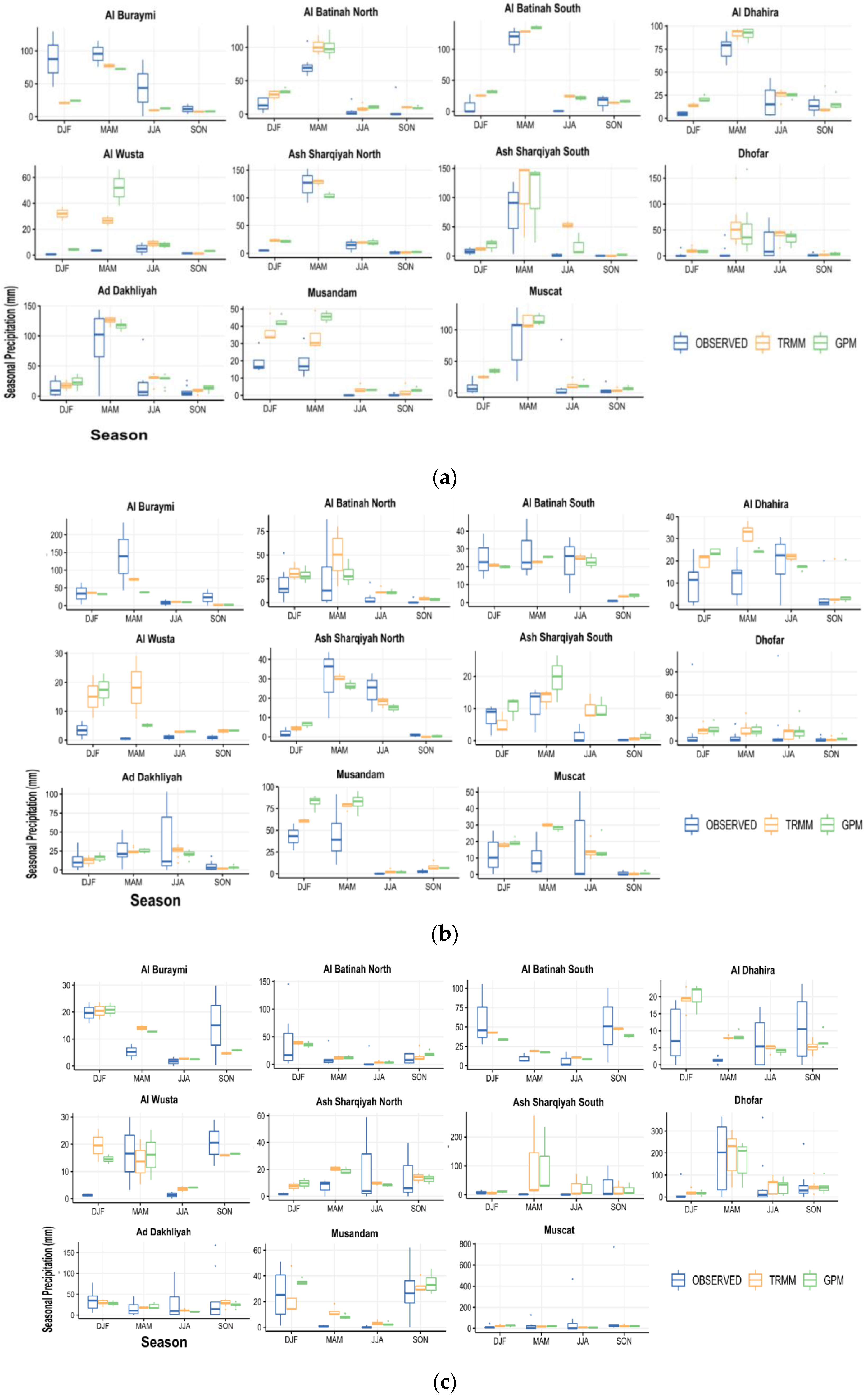
Figure 7 shows the box and whisker plot of the satellite products and OBSERVED across the 11 governorates of Oman for (a) 2016, (b) 2017, and (c) 2018. The governorates received different amounts of precipitation during the study period; as such, Figure 7 shows clear spatial variability and heterogeneity in terms of the frequency and amount of rain received by each governorate. It is notable that although the governorates have different climatic regions (coastal, mountainous, desert plain, etc.), across the country, the spring season had the highest amount of precipitation and the largest variability. The only exception was the Dhofar Governorate, where a large amount of precipitation occurred in the summer during the Kharif season mentioned above.
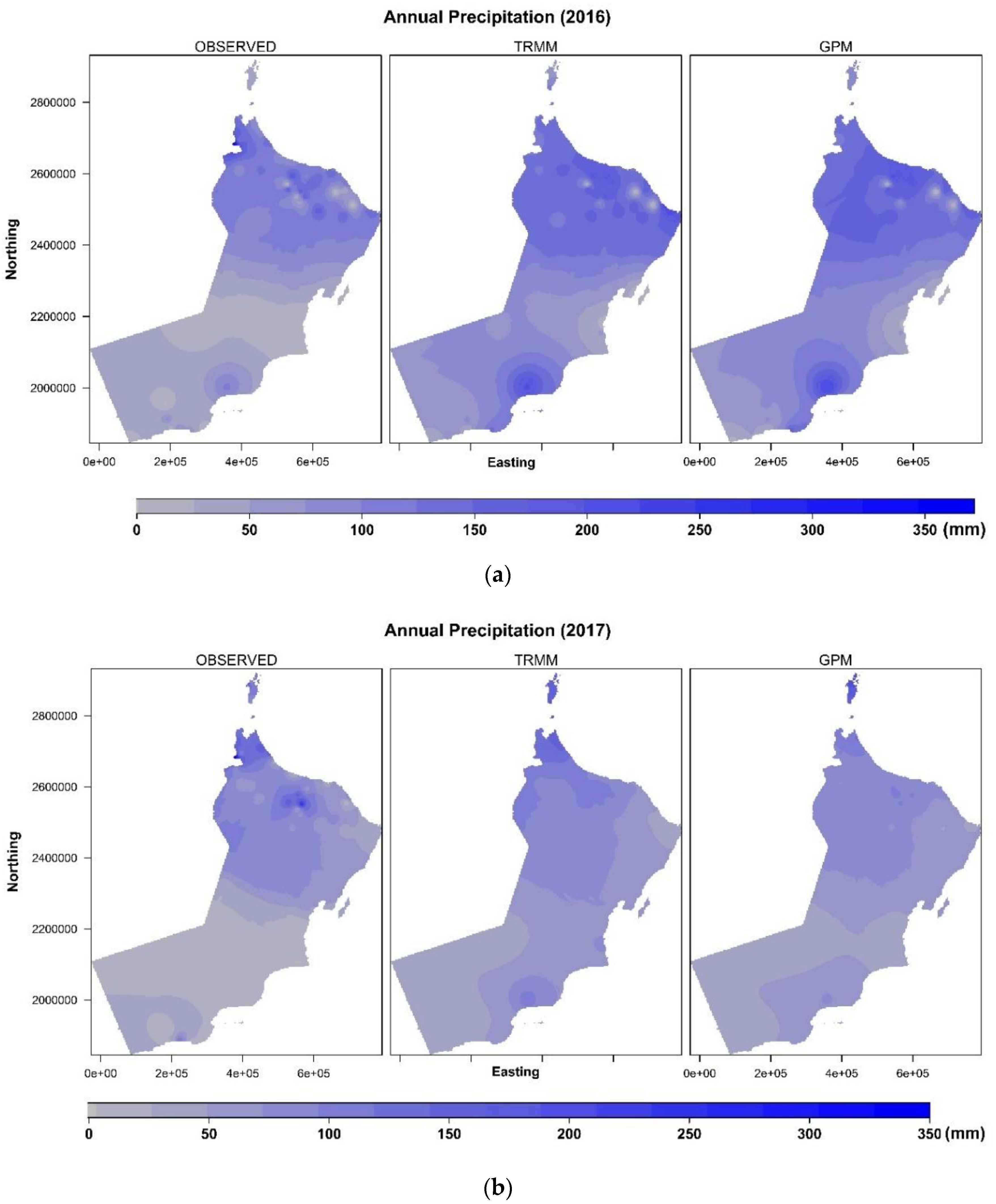
Figure 8 shows the spatial distribution of annual precipitation for Oman, 2016 (a), 2017 (b), and 2018 (c). There was a clear trend in the distribution of precipitation across the country, with high values observed in the northern part of Oman and low values in the southern and interior parts. This finding was consistent across the three study years. The impact of the Mekunu cyclone and Lubia tropical storm elevated the annual values shown in 2018. Moreover, there were no striking differences between the TRMM and GPM estimates in either year.

3.3. Assessments of GPM and TRMM using Continuous Verification Indices

Table 5 shows the RMSE and AME values for the entire country and the three precipitation regimes. TRMM and GPM have an RMSE of 37.13 and 36.68 mm/month, respectively. Both products also have a similar MAE of approximately 9 mm/month. This similarity and trend were noticed in all the three different precipitation regimes of Oman. Notably, the RMSE values of both products in the Dhofar region were higher than the entire country. This region experienced a cyclone and tropical storms in two of the years (2017 and 2018). These large values may be a result of both TRMM and GPM underestimating these extreme events.
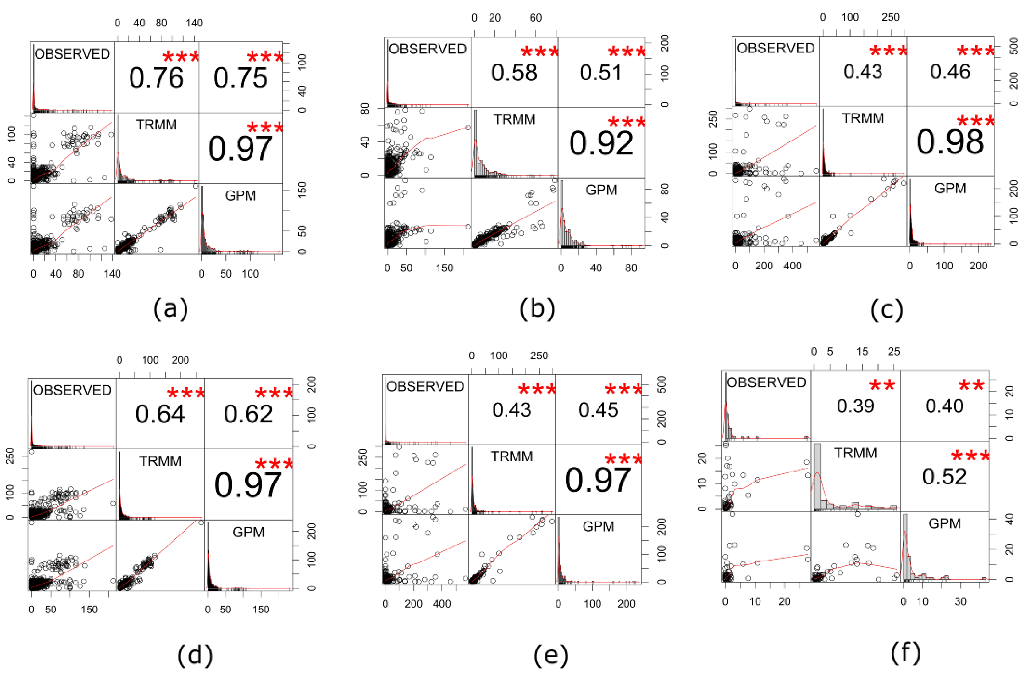
Figure 9 shows the correlation matrix of the monthly average precipitation of TRMM, GPM, and OBSERVED for year (a) 2016, (b) 2017, and (c) 2018 and for subdivisions (d) Northern, (e) Dhofar, and (f) Interior of Oman. The estimates of both GPM and TRMM were correlated with the OBSERVED, with values of r = 0.76 and 0.75 for TRMM and GPM, respectively, for 2016, demonstrating good agreement. The GPM and TRMM estimates were also correlated (r > 0.97), suggesting that GPM is a suitable replacement for TRMM and also confirming the similarities in their underlying algorithm. For cyclone years (2017 and 2018), there were weak correlations that suggest there is a misalignment in the 1:1 relationship between the OBSERVED and satellite products. Figure 9d–f are scatterplots showing the correlation between satellite products and OBSERVED for three subdivisions of Oman. As shown in Figure 9d, in the Northern region of Oman, the two satellite products showed good agreement with OBSERVED estimates, with correlation values of r = 0.64 and 0.62 for TRMM and GPM, respectively. In contrast, the performance of both satellite products was weak in the Dhofar region (Figure 9e). Indeed, correlation with the OBSERVED was weaker, with values of r = 0.43 and 0.45 for TRMM and GPM, respectively. The distribution of the station data around the correlation line was also highly variable. It is important to note that the Dhofar region includes both mountainous and coastal areas. Further research may be needed to better understand the performance of satellite observations for these distinct climatic regions. Weaker correlations were also shown for the Interior region with r = 0.39 and 0.40 for TRMM and GPM, respectively.

3.4. Performance Assessments of GPM and TRMM Using Change Point Analysis

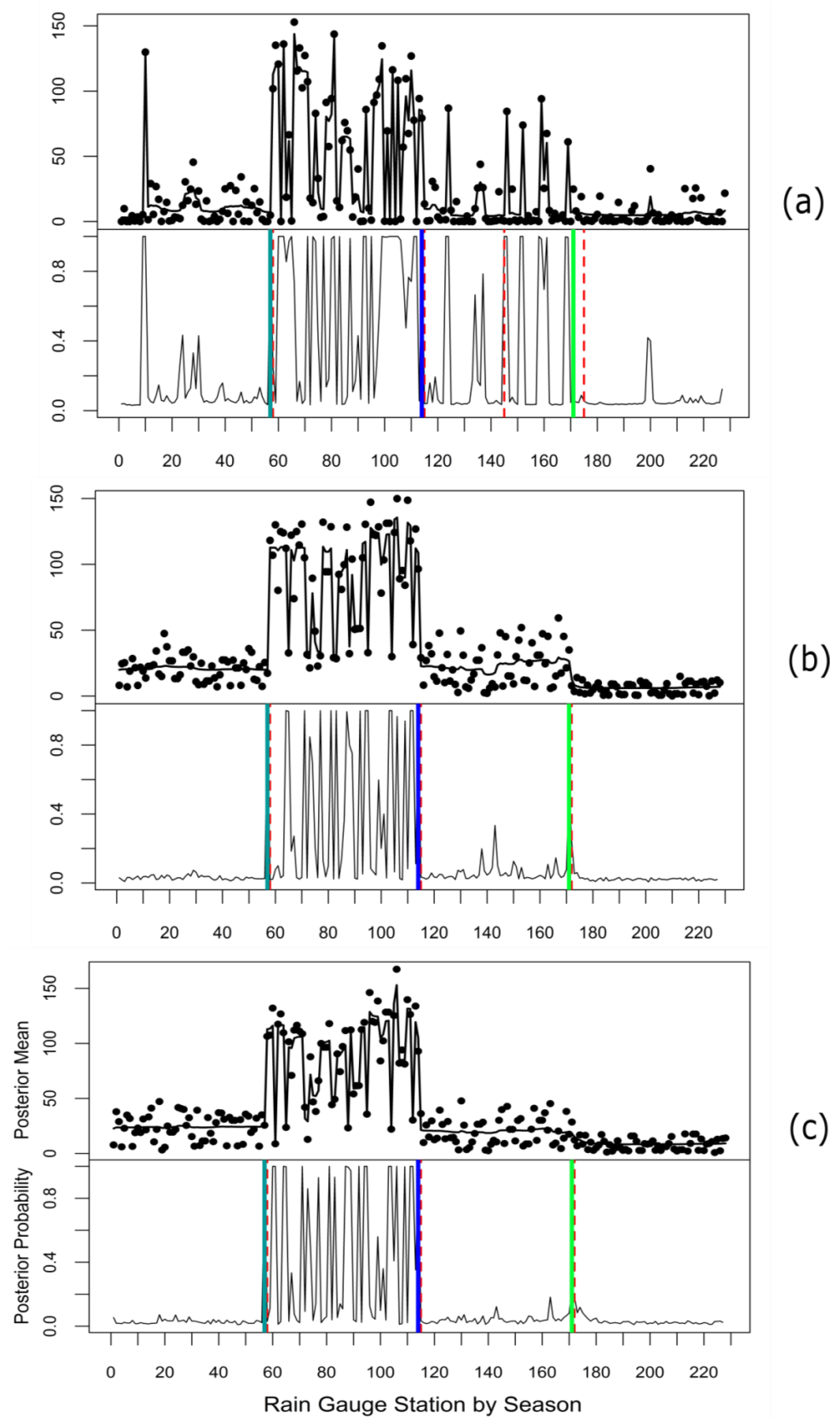
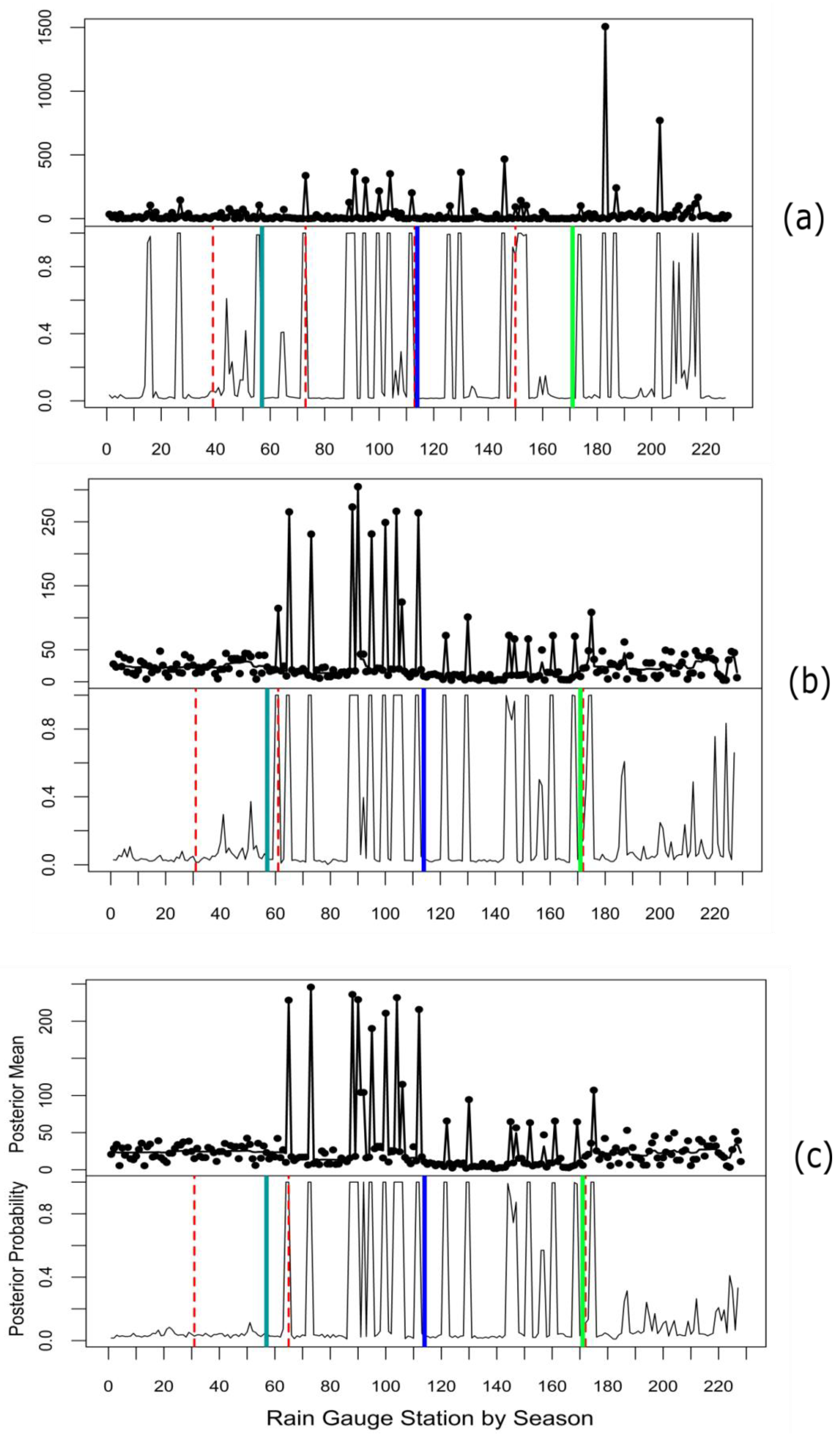
The change point plots in Figure 10, Figure 11 and Figure 12 show the partitioning of the original seasonal datasets (solid lines) and location of change and aberrations with high posterior probability (dash red lines) identified by both the bcp and ecp methods. In Figure 10, change point methods clearly differentiate the seasonal pattern in OBSERVED, TRMM, and GPM for 2016, except the extract change points at locations 142 and 173 identified in OBSERVED. This may be a result of “more noise” in OBSERVED compared to TRMM and GPM, which were from gridded products. Interpolated/gridded surfaces tend to smoothing values through the underestimation of high values and overestimation of low values. In general, it is clear that TRMM and GPM have similar internal structures compared to the OBSERVED time series from the perspective of the seasonal changes. For 2017 (Figure 11), it is clear that the satellite products show similar characteristics compared to the OBSERVED, as there were change points that did not follow the original seasonal changes. The timing and locations of changes in both observed and satellite products look similar. This also shows that satellite products exhibit similar seasonal properties of the OBSERVED for 2017. In Figure 12, OBSERVED and satellite products show similar change points that did not follow the original seasonal partitioning. The posterior probabilities of change at each of the changing locations are similar for both OBSERVED and the satellite products. The seasonal response and timing of any precipitation products are paramount as properties to be considered in seasonal forecast, hydrologic modeling and river basin water balance analysis.

3.5. Performance Assessments of GPM and TRMM Using Categorical Verification Indices

Figure 13 shows a performance diagram of TRMM and GPM at different precipitation thresholds for the year (a) 2016, (b) 2017, and (c) 2018 and for subdivisions (d) Northern, (e) Dhofar and (f) Interior of Oman. This diagram provides several categorical indexes (POD, BIAS, CSI, and SR (1-FAR)) together on a single page. The five different precipitation thresholds are considered and represented from the smallest (2 mm/month) to the largest (>30 mm/month). The solid contour lines show the CSI values, while the BIAS shows the dash lines with extended labels on the upper (2nd) axes of x and y. In all the considered scenarios, it is clear that TRMM (red) and GPM (green) produced high POD (>0.8) at low precipitation thresholds. POD decreased as precipitation thresholds increased, except for the case shown in Figure 13a. It is interesting to see that TRMM and GPM performed well in 2016 (Figure 13a). This is the only year without any major tropical storm or cyclone events. In 2016, both TRMM and GPM detected large precipitation (>30 mm/month), low CSI, and BIAS of 1. Tropical cyclones are always characterized by high winds, intense rainfall, warm temperatures, and low atmospheric pressures. It seems both TRMM and GPM have problems detecting these features compared to a period when there are no such events. This result is consistent with performance using other techniques such as change point and correlation. In Figure 13b,c, it is shown that TRMM and GPM have problems detecting large amounts of precipitation and also underestimate large precipitation thresholds. For the three regions considered, TRMM and GPM show similar performance of overestimation of low precipitations and underestimation of large precipitations. In terms of BIAS (frequency bias), TRMM slightly performed better than GPM at low and high precipitation thresholds. TRMM’s CSI was similar to GPM at low and high thresholds (>30 mm/month). In terms of SR (i.e., 1-FAR), the two products performed similarly.
Figure 13e shows the performance diagram of the satellite products for the Dhofar Region. TRMM and GPM performed similarly in detecting precipitation at the defined precipitation thresholds. The performance of both TRMM and GPM are shown in Figure 13f for the Interior Region. In this region, both products had difficulty detecting high precipitation levels. However, it is important to note that this region has the fewest rain gauge stations, which may have an influence on or inflate this “similar” result.
This study evaluated the strength and weaknesses of two satellite products for Oman. In general, both satellites use the same algorithm and therefore not surprising the similarities in performance. From the literature, previous studies such as those by Zhang et al. [18] and Tan and Duan [47] did not observe any significant improvement of GPM over TRMM. The result from this study is also consistent with findings from African coastal [48] and high topography [49] areas, where issues with the performance of satellite observations have been reported. While TRMM will be completely discontinued, GPM has better spatial and temporal resolutions with potential applications such as in operational cyclone monitoring in Oman. This study is very important and relevant for regions with sparse rain gauge networks. The steps applied for this evaluation may be applied to other areas but care must be taken when applying to regions with a different number of rain gauge networks and contrast climatic characteristics.

3.6. Importance of Precipitation Estimates and Analysis in Socio-Hydrologic Resilience

For a country like Oman, which is prone to frequent extreme events such as cyclones, sea-level rise, flash floods, etc., the importance of precipitation measurement and analysis cannot be over-emphasized. These events cannot be stopped from occurring, but they can be adapted to. In the face of these frequent threatening events, decision-makers, farmers, and all stakeholders need a decision support tool that can provide timely information about precipitation values in near real-time. There is a need to utilize currently available satellite precipitation products and OBSERVED in an integrated way for sustainable water management, flood and seasonal forecasting, hydrologic modeling, etc. Beyond the usefulness of satellite observations, there is a need for pragmatic efforts in providing a platform for precipitation analysis that has both finer spatial and temporal resolutions. Creating this platform is possible through the assimilation of climatic forecast (as a first guess), OBSERVED, satellite and radar rainfall observations, similar to the Canadian Precipitation Analysis [8,50,51]. With an appropriate bias correction framework such as that which is implemented in Friesen et al. [52], this method will correct and adjust the precipitation intensity and systematic bias. In other words, for real-time or near real-time applications, the average monthly accumulated OBSERVED from rain gauges through the entire country (from the previous 30 days) can be used for bias correction. The evaluated satellite products can be used as an additional data source or as a background field. The rainfall analysis could be produced either at 6-h or daily time steps. Having this type of product would strengthen Oman’s adaptive strategies and socio-hydrologic resilience, especially in combating frequent extreme events.

4. Conclusions

This study evaluated the accuracy of precipitation estimates produced by two satellite products: TRMM (3B43V7) and GPM (IMERG V6) in the Sultanate of Oman. For continuous statistics verification performance, indices such as correlation ( r ), RMSE, and MAE were used to compare the association between the satellite products and OBSERVED from 77 weather stations. In the categorical verification domain, statistics such as CSI, SR (i.e., 1-FAR), POD, and BIAS (frequency bias) were used to assess the performance of the two products. In addition, change point methods from the Bayesian and non-parametric perspectives were also used to determine the timing and number of changes in the time-series. Study findings indicated that both GPM and TRMM compared well with OBSERVED observations in 2016, when there was no tropical storm or cyclone. It is recommended that future studies investigate the performance of early runs of GPM for real-time extreme events such as cyclone monitoring in Oman. However, before using these products for operational applications, relevant bias correction procedures may be needed. Additionally, more study years should be evaluated if OBSERVED from more rain-gauge stations is available. For hydrological forecasting or agricultural applications such as capturing near real-time cyclones, the satellite products should be assessed at shorter temporal scales such as sub-hourly, hourly, or daily accumulated rates.
In the current study, the following concluding remarks were drawn:
(1)
There was generally a weak linear relationship between GPM and TRMM in all the regions and years considered for the entire period of study, except for the good correlation observed in the Northern region and also in 2016 (for the entire country). The year 2016 was without any cyclone event and was generally dry except for heavy rain in March 2016. The weak performances seen in the Dhofar region may be due to the two distinct physiographic features in the areas (mountain and coastal climates). The Dhofar region may need to be analyzed separately in future studies to more accurately assess the performance of the satellite products in the region. Examining the products across all 11 governorates of Oman, there was consistent spatial variability in the satellite products, especially in regions where there are relatively few gauged networks. Bias corrections may be needed to be performed on the products before being used for any real-time applications.
(2)
In Oman, both products can detect low to medium precipitation thresholds; however, both have difficulty detecting precipitations at higher thresholds. In terms of BIAS, both products overestimated precipitation compared to OBSERVED at low precipitation thresholds, but underestimated precipitation levels at high thresholds. Of the three regions considered, there was a similar performance of the satellite products in all the regions, confirming the similarities in the algorithms used to produce them. For all the regions, the weak correlation performances noted above also reflect in the categorical performance.
(3)
From the change point analysis perspective, TRMM and GPM compared well with OBSERVED in their ability to detect seasonal changes or aberrations in both annual and seasonal scales. Although there were differences in terms of the posterior mean obtained from bcp, there were similarities in change points or aberrations in the rain-gauge station locations across all the years. In general, TRMM and GPM showed similar characteristics with the OBSERVED in the number and timing of seasonal changes computed across the years.
(4)
In terms of measuring annual precipitation, the two satellite products demonstrated the same spatial pattern as the OBSERVED over the three study years (except 2018, when there was a tropical storm and a cyclone). In all the years, there was strong agreement between TRMM and GPM in terms of spatial distribution and magnitude.
Overall, this study assessed the performance of the GPM and TRMM satellite products in Oman. Both showed promising results (which can further be improved with appropriate bias corrections) in terms of acting as proxies for OBSERVED. There were no marked differences between the two products, suggesting that GPM can act as a reliable replacement for TRMM.

Funding

The author would like to thank the Dean’s Seed Fund, College of Agriculture and Marine Science, Sultan Qaboos University, Muscat, Oman (Grant No: IG/AGR/DEAN/19/01) for providing the funding in support of this research.

Acknowledgments

Constructive suggestions from the Academic Editor and three anonymous reviewers are appreciated.

Conflicts of Interest

The author declares that no conflict of interest could have influenced the findings of this paper.

References

  1. Chung-Chen, J.; Kot, S.C.; Tepper, M. Comparing NOAA-12 and Radiosonde Atmospheric Sounding Profiles for Mesoscale Weather Model Initialization. In COSPAR Colloquia Series; Elsevier: Amsterdam, The Netherlands, 1997; pp. 103–109. [Google Scholar] [CrossRef]
  2. Food and Agriculture Organization. Climate Change and Food Security: A Framework Document; Food and Agriculture Organization of the United Nations (FAO): Rome, Italy, 2008; Available online: www.fao.org/forestry/15538-079b31d45081fe9c3dbc6ff34de4807e4.pdf (accessed on 26 May 2020).
  3. Ballester, J.; More, J. The representativeness problem of a station net applied to the verification of a precipitation forecast based on areas. Meteorol. Appl. 2007, 14, 177–184. [Google Scholar] [CrossRef]
  4. Saulo, A.C.; Ferreira, L. Evaluation of quantitative precipitation forecasts over southern South America. Aust. Meteorol. Mag. 2003, 52, 81–93. [Google Scholar]
  5. Tustison, B.; Harris, D.; Foufoula-Georgiou, E. Scale issues in verification of precipitation forecasts. J. Geophys. Res. 2001, 106, 11775–11784. [Google Scholar] [CrossRef]
  6. Directorate General of Meteorology and Air Navigation (2012). Annual Report on Activities in Meteorology. National Report submitted to the Panel on Tropical Cyclones in the Bay of Bengal and Arabian Sea. In Proceedings of the 39th Session, Nay Pye Taw, Myanmar, 5–9 February 2012; Available online: https://www.wmo.int/pages/prog/www/tcp/documents/Oman.doc (accessed on 20 January 2020).
  7. WMO. Guide to Hydrological Practices. Volume I. Hydrology-From Measurement to Hydrological Information. WMO-No. 168, 6th ed.; WMO: Geneva, Switzerland, 2008. Available online: http://www.wmo.int/pages/prog/hwrp/publications/guide/english/168_Vol_I_en.pdf (accessed on 22 December 2019).
  8. Boluwade, A.; Stadnyk, T.; Fortin, V.; Roy, G. Assimilation of precipitation Estimates from the Integrated Multisatellite Retrievals for GPM (IMERG, early Run) in the Canadian Precipitation Analysis (CaPA). J. Hydrol. Reg. Stud. 2017, 14, 10–22. [Google Scholar] [CrossRef]
  9. Huffman, G.J.; Adler, R.F.; Bolvin, D.T.; Nelkin, E.J. The TRMM Multi-satellite Precipitation Analysis (TMPA). Chapter 1. In Satellite Rainfall Applications for Surface Hydrology; Springer: Dordrecht, The Netherlands, 2010; pp. 3–22. [Google Scholar] [CrossRef]
  10. Horishima, K. Rainfall observation from Tropical Rainfall Measuring Mission (TRMM) satellite. J. Vis. 1999, 2, 93–98. [Google Scholar] [CrossRef]
  11. Flaming, G.M. Measurement of global precipitation. In Proceedings of the 2004 IEEE International Geoscience and Remote Sensing Symposium (IGARSS 2004), Anchorage, AK, USA, 20–24 September 2004; IEEE: New York, NY, USA, 2004. [Google Scholar] [CrossRef]
  12. Kummerow, C.J.; Simpson, O.; Thiele, W.; Barnes, A.T.; Chang, E.; Stocker, R.F.; Adler, A.; Hou, R.; Kakar, F.; Wentz, P.; et al. The Status of the Tropical Rainfall Measuring Mission (TRMM) after Two Years in Orbit. J. Appl. Meteor. 2000, 39, 1965–1982. [Google Scholar] [CrossRef]
  13. Tropical Rainfall Measuring Mission (TRMM). TRMM (TMPA/3B43) Rainfall Estimate L3 1 Month 0.25 Degree × 0.25 Degree V7; Goddard Earth Sciences Data and Information Services Center (GES DISC): Greenbelt, MD, USA, 2011. Available online: https://disc.gsfc.nasa.gov/datasets/TRMM_3B43_7/summary (accessed on 3 March 2020). [CrossRef]
  14. Yuan, F.; Wang, B.; Shi, C.; Cui, W.; Zhao, C.; Liu, Y.; Ren, L.; Zhang, L.; Zhu, Y.; Chen, T.; et al. Evaluation of hydrological utility of IMERG Final run V05 and TMPA 3B42V7 satellite precipitation products in the Yellow River source region, China. J. Hydrol. 2018, 567, 696–711. [Google Scholar] [CrossRef]
  15. Silva Lelis, L.C.; Duarte Bosquilia, R.W.; Duarte, S.N. Assessment of Precipitation Data Generated by GPM and TRMM Satellites. Rev. Bras. Meteorol. 2018, 33, 153–163. [Google Scholar] [CrossRef] [Green Version]
  16. Rozante, J.R.; Vila, D.A.; Chiquetto, J.B.; Fernandes, A.A.; Alvim, D.S. Evaluation of TRMM/GPM Blended Daily Products over Brazil. Remote Sens. 2018, 10, 882. [Google Scholar] [CrossRef] [Green Version]
  17. Xu, R.; Tian, F.Q.; Yang, L.; Hu, H.C.; Lu, H.; Hou, A.Z. Ground validation of GPM IMERG and TRMM 3B42V7 rainfall products over southern Tibetan Plateau based on a high-density rain gauge network. J. Geophys. Res. Atmos. 2017, 122, 910–924. [Google Scholar] [CrossRef]
  18. Zhang, S.; Wang, D.; Qin, Z.; Zheng, Y.; Guo, J. Assessment of the GPM and TRMM Precipitation Products Using the Rain Gauge Network over the Tibetan Plateau. J. Meteorol. Res. 2018, 32, 324. [Google Scholar] [CrossRef]
  19. Boluwade, A.; Zhao, K.Y.; Stadnyk, T.A.; Rasmussen, P. Towards Validation of the Canadian Precipitation Analysis (CaPA) for Hydrologic Modeling Applications in the Canadian Prairies. J. Hydrol. 2018, 556. [Google Scholar] [CrossRef]
  20. Matteson, D.S.; James, N.A. A Nonparametric Approach for Multiple Change Point Analysis of Multivariate Data. J. Am. Stat. Assoc. 2014, 109, 334–345. [Google Scholar] [CrossRef] [Green Version]
  21. Erdman, C.; Emerson, J.W. A fast Bayesian change point analysis for the segmentation of microarray data. Bioinformatics 2008, 24, 2143–2148. [Google Scholar] [CrossRef] [PubMed] [Green Version]
  22. Eslamiana, S.; Naser, M.; Symec, R.G. Building socio-hydrological resilience: From theory to practice. J. Hydrol. 2019, 575, 930–932. [Google Scholar] [CrossRef]
  23. Kwarteng, A.Y.; Dorvlo, A.S.; Vijaya Kumar, G.T. Analysis of a 27-year rainfall data (1977–2003) in the Sultanate of Oman. Int. J. Climatol. 2009, 29, 605–617. [Google Scholar] [CrossRef]
  24. Al-Shaqsi, S. Care or Cry: Three years from Cyclone Gonu. What have we learnt? OMJ 2010, 25, 162–167. Available online: http://www.omjournal.org/OriginalArticles/FullText/201007/FT_CareorCry.html (accessed on 22 December 2019). [CrossRef]
  25. India Meteorological Department (January 2008). “Report on Cyclonic Disturbances over North Indian Ocean during 2007”. Archived from the Original on 26 November 2008. Retrieved 18 April 2010. Available online: https://www.webcitation.org/5ccClL6ET?url=http://sonicfighters.com/rattleman/other/tropics/IMD_2007_Report_HTML.html (accessed on 22 December 2019).
  26. Masters, J. Earth’s 39 Billion-Dollar Weather Disasters of 2018: 4th-Most on Record. 2019. Available online: https://www.wunderground.com/cat6/Earths-39-Billion-Dollar-Weather-Disasters-2018-4th-Most-Record (accessed on 22 December 2019).
  27. Adler, R.F.; Huffman, G.J.; Bolvin, D.T.; Curtis, S.; Nelkin, E.J. Tropical rainfall distributions determined using TRMM combined with other satellite and rain gauge information. J. Appl. Meteorol. 2000, 39, 2007–2023. [Google Scholar] [CrossRef] [Green Version]
  28. Chiu, L.S.; Liu, Z.; Rui, H.; Teng, L.W. TRMM data and Access Tools. In Earth Science Satellite Remote Sensing; Qu, J.J., Gao, W., Kafatos, M., Murphy, R.E., Salomonson, V.V., Eds.; Springer and Tsinghua University Press: Beijing, China, 2006; pp. 202–219. [Google Scholar]
  29. Nicholson, S.E.B.; Some, J.; McCollum, E.; Nelkin, D.; Klotter, Y.; Berte, B.M.; Diallo, I.; Gaye, G.; Kpabeba, O.; Ndiaye, J.N.; et al. Validation of TRMM and Other Rainfall Estimates with a High-Density Gauge Dataset for West Africa. Part I: Validation of GPCC Rainfall Product and Pre-TRMM Satellite and Blended Products. J. Appl. Meteorol. 2003, 42, 1337–1354. [Google Scholar] [CrossRef]
  30. Liu, Z. Comparison of Integrated Multisatellite Retrievals for GPM (IMERG) and TRMM Multisatellite Precipitation Analysis (TMPA) Monthly Precipitation Products: Initial Results. J. Hydrometeorol. 2016, 17. [Google Scholar] [CrossRef]
  31. Schmidt, E.J.; Schulze, R.E. Flood Volume and Peak Discharge from Small Catchments in Southern Africa Based on the SCS Technique; WRC Report No. TT 31/8; Water Research Commission: Pretoria, South Africa, 1987; p. 164. [Google Scholar]
  32. Dent, M.C.; Lynch, S.D.; Schulze, R.E. Mapping Mean Annual and Other Rainfall Statistics Over Southern Africa; Agricultural Research Unit Report No. 27; University of Natal: Pietermaritzburg, South Africa, 1987. [Google Scholar]
  33. Arteaga-Ramirez, R.; Tijerina-Chavez, L.; Valdez-Cepeda, R.D.; Vazquez-Pena, M.A.; Mejia-Saenz, E. Temporal and spatial representativeness of the information of extreme temperatures in a network of meteorological stations in Guanajuato, Mexico. Ing. Hidraul. Mexico 2004, 19, 53–64. [Google Scholar]
  34. Hou, A.Y.; Skofronick-Jackson, G.; Kummerow, C.D.; Shepherd, J.M. Global Precipitation Measurement. Part II: Precipitation: Advances in Measurement, Estimation and Prediction; Springer: Berlin/Heidelberg, Germany, 2008; pp. 131–169. [Google Scholar] [CrossRef] [Green Version]
  35. Huffman, G.J.; Bolvin, D.T.; Nelkin, E.J. Integrated Multi-Satellite Retrievals for GPM (IMERG) Technical Documentation; NASA/GSFC: Greenbelt, MD, USA, 2017.
  36. Tan, J.; Petersen, W.A.; Kirstetter, P.E.; Tian, Y.D. Performance of IMERG as a function of spatio-temporal scale. J. Hydrometeorol. 2017, 18, 307–319. [Google Scholar] [CrossRef] [PubMed]
  37. Becker, A. The Global Precipitation Climatology Centre (GPCC) to Support the GCW on ECV Precipitation: Caps and Constrains. In Proceedings of the 1st GCW Implementation Meeting, Geneva, Switzerland, 21–24 November 2011; pp. 1–40. Available online: https://www.wmo.int/pages/prog/www/OSY/Meetings/GCW-IM1/Doc12.4_GPCC.pdf (accessed on 4 December 2019).
  38. World Climate Research Programme (WCRP). WWRP/WGNE Joint Working Group on Forecast Verification Research. Forecast Verification Methods Across Time and Space Scales; WCRP: Berlin, Germany, 2017. Available online: https://www.cawcr.gov.au/projects/verification/ (accessed on 22 December 2019).
  39. World Meteorological Organization. Chapter 14. Observation of present and past weather; state of the ground. In Guide to Meteorological Instruments and Methods of Observation; WMO: Geneva, Switzerland, 2012; pp. 14–19. [Google Scholar]
  40. Llasat, M.C. An objective classification of rainfall events on the basis of their convective features: Application to rainfall intensity in the northeast of Spain. Int. J. Climatol. 2001, 21, 1385–1400. [Google Scholar] [CrossRef]
  41. Roebber, P.J. Visualizing multiple measures of forecast quality. Weather Forecast. 2009, 24, 601–608. [Google Scholar] [CrossRef] [Green Version]
  42. Gilleland, M.E. Package ‘Verification’. Available online: http://cran.utstat.utoronto.ca/web/packages/verification/verification.pdf (accessed on 25 September 2019).
  43. Boluwade, A. Regionalization and Partitioning of Soil Health Indicators for Nigeria Using Spatially Contiguous Clustering for Economic and Social-Cultural Developments. ISPRS Int. J. Geo-Inform. 2019, 8, 458. [Google Scholar] [CrossRef] [Green Version]
  44. Vostrikova, L. Detection Disorder in Multidimensional Random Processes. Sov. Math. Dokl. 1981, 24, 55–59. [Google Scholar]
  45. Sz’ekely, G.J.; Rizzo, M.L. Hierarchical Clustering via Joint Between-Within Distances: Extending Ward’s Minimum Variance Method. J. Classif. 2005, 22, 151–183. [Google Scholar] [CrossRef]
  46. Floodlist, Oman. Oman and Yemen—Tropical Cyclone ‘Luban’ Leaves 3 Dead. Available online: http://floodlist.com/tag/oman (accessed on 22 December 2019).
  47. Tan, M.; Duan, Z. Assessment of GPM and TRMM Precipitation Products over Singapore. Remote Sens. 2017, 9, 720. [Google Scholar] [CrossRef] [Green Version]
  48. Toté, C.; Patricio, D.; Boogaard, H.; Van der Wijngaart, R.; Tarnavsky, E.; Funk, C. Evaluation of Satellite Rainfall Estimates for Drought and Flood Monitoring in Mozambique. Remote Sens. 2015, 7, 1758–1776. [Google Scholar] [CrossRef] [Green Version]
  49. Yin, Z.Y.; Zhang, X.; Liu, X.; Colella, M.; Chen, X. An assessment of the biases of satellite rainfall estimates over the Tibetan Plateau and correction methods based on topographic analysis. J. Hydrometeorol. 2008, 9, 301–326. [Google Scholar] [CrossRef]
  50. Lespinas, F.; Fortin, V.; Roy, G.; Rasmussen, P.; Stadnyk, T. Performance evaluation of the canadian precipitation analysis (CaPA). J. Hydrometeor. 2015, 16, 2045–2064. [Google Scholar] [CrossRef]
  51. Fortin, V.; Roy, G.; Donaldson, N.; Mahidjiba, A. Assimilation of radar quantitative precipitation estimations in the Canadian Precipitation Analysis (CaPA). J. Hydrol. 2015, 531, 296–307. [Google Scholar] [CrossRef]
  52. Friesen, B.; Boluwade, A.; Rasmussen, P.F.; Fortin, V. Assimilation of satellite-based rainfall estimations in the Canadian precipitation analysis. J. Hydrol. Eng. 2017, 22, 04017049. [Google Scholar] [CrossRef]
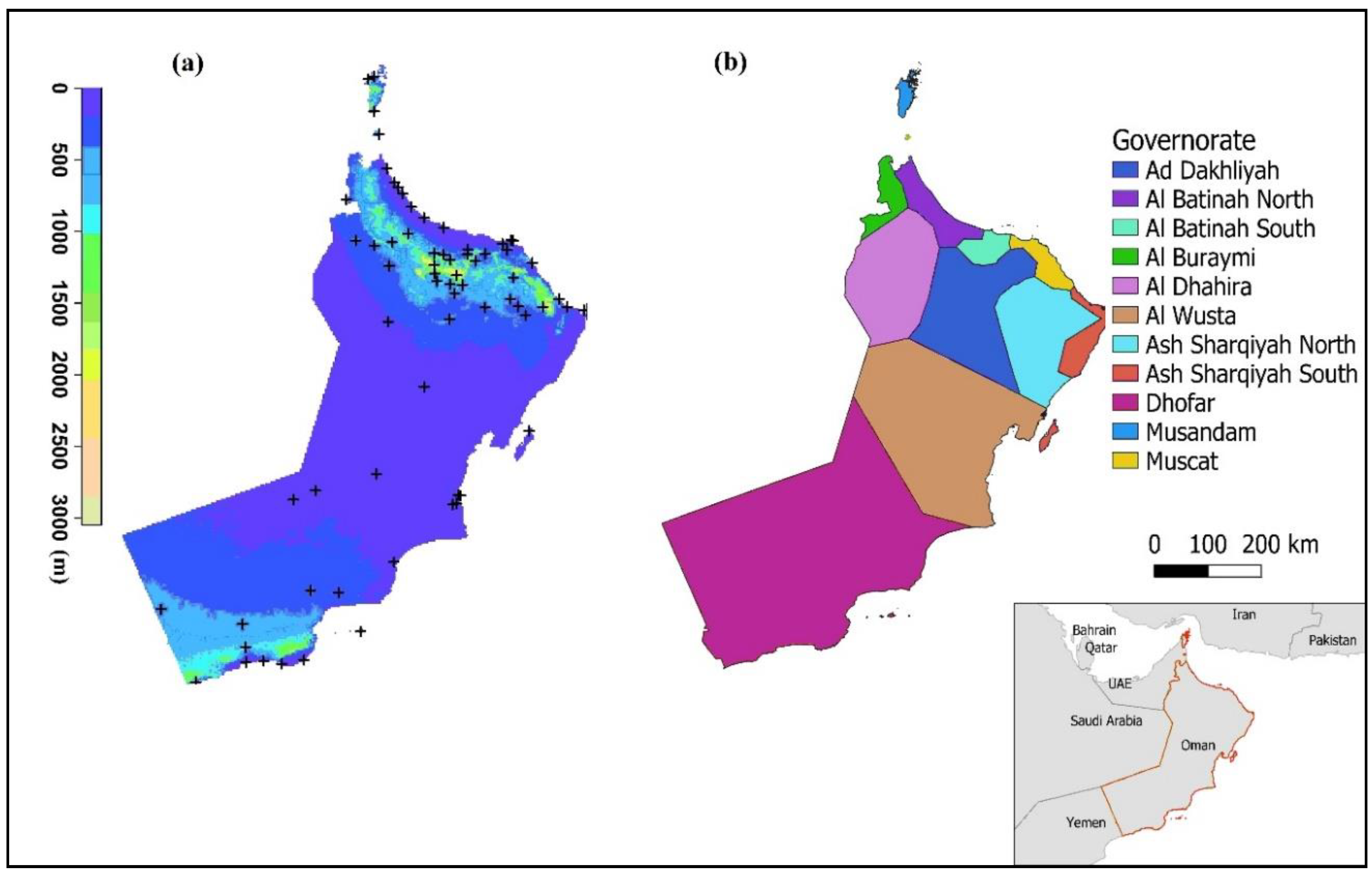
Figure 1. Map of the Sultanate of Oman showing the rain-gauge stations, (a) elevation and (b) 11 governorates. The points with cross signs indicate rain-gauge locations.
Atmosphere 11 00901 g001
Figure 2. Rain gauge station locations and subdivisions of the study area classified by Oman’s rainfall pattern.
Atmosphere 11 00901 g002
Figure 3. Visual representation of the missing monthly precipitation values from 2008–2018. The missing and observed (present) values are represented by yellow and navy-blue respectively.
Atmosphere 11 00901 g003
Figure 4. Monthly averages of precipitation estimates from NCSI (OBSERVED, (blue)), Global Precipitation Measurement (GPM) (green), and Tropical Rainfall Measuring Mission (TRMM) (red)) in Oman (2016–2018).
Atmosphere 11 00901 g004
Figure 5. Regional monthly averages of precipitation estimates from gauged and satellite products for (a) entire country, (b) Dhofar, (c) Interior, and (d) Northern region for 2016–2018. OBSERVED, Tropical Rainfall Measuring Mission (TRMM), and Global Precipitation Measurement (GPM) are in blue, red, and green, respectively. Months are the axes (anti-clockwise), and the values on the axes are monthly precipitation (mm/month).
Atmosphere 11 00901 g005
Figure 6. Seasonal averages of precipitation estimates from NCSI (OBSERVED, (blue)), GPM (green), and TRMM (red) for the entire country in (a) 2016, (b) 2017, and (c) 2018. Monthly precipitation data were accumulated into the season time scale as: spring (MAM: March, April, and May), summer (JJA: June, July, and August), and fall (SON, September, October, and November).
Atmosphere 11 00901 g006
Figure 7. Seasonal averages of precipitation estimates from NCSI (OBSERVED, (blue)), GPM (green), and TRMM (orange)) across the 11 governorates of Oman for (a) 2016, (b) 2017, and (c) 2018.
Atmosphere 11 00901 g007
Figure 8. Spatial distribution and variability of annual precipitation from the rain gauge stations and satellite products in Oman, 2016 (a), 2017 (b), and 2018 (c).
Atmosphere 11 00901 g008aAtmosphere 11 00901 g008b
Figure 9. Scatterplot matrix showing the histograms, kernel density overlays, absolute correlation and significance levels (*** p < 0.001) between OBSERVED, TRMM, and GPM precipitation estimates for the year (a) 2016, (b) 2017, and (c) 2018 and region (d) Northern, (e) Dhofar, and (f) Interior.
Atmosphere 11 00901 g009
Figure 10. Bayesian change point (bcp) and nonparametric approach for multiple change point analysis (ecp) results for 2016 (seasonal accumulation) for (a) OBSERVED, (b) TRMM, and (c) GPM. The solid lines show the original seasonal partitioning season (the teal color indicates when DJF (winter) ends and spring (MAM) begins, the blue color when spring ends and summer (JJA) begins, and green when summer ends and autumn (SON) begins). The dash red lines show the change points derived using both bcp and ecp. The X-axis indicates the total number of rain-gauge stations (57) used, meaning each partition (solid line and season) has 57 stations.
Atmosphere 11 00901 g010
Figure 11. Bayesian change point (bcp) and nonparametric approach for multiple change point analysis (ecp) results for 2017 (seasonal accumulation) for (a) OBSERVED, (b) TRMM, and (c) GPM. The solid lines show the original seasonal partitioning season (the teal color indicates when DJF (winter) ends and spring (MAM) begins, the blue color when spring ends and summer (JJA) begins, and green when summer ends and autumn (SON) begins). The dash red lines show the change points derived using both bcp and ecp. The X-axis indicates the total number of rain-gauge stations (57) used, meaning each partition (solid line and season) has 57 stations.
Atmosphere 11 00901 g011
Figure 12. Bayesian change point (bcp) and nonparametric approach for multiple change point analysis (ecp) results for 2018 (seasonal accumulation) for (a) OBSERVED, (b) TRMM, and (c) GPM. The solid lines show the original seasonal partitioning season (the teal color indicates when DJF (winter) ends and spring (MAM) begins, the blue color when spring ends and summer (JJA) begins, and green when summer ends and autumn (SON) begins). The dash red lines show the change points derived using both bcp and ecp. The X-axis indicates the total number of rain-gauge stations (57) used, meaning each partition (solid line and season) has 57 stations.
Atmosphere 11 00901 g012
Figure 13. Categorical verification technique (performance diagram) showing the Success Ratio (SR), Probability of Detection (POD), BIAS, and CSI values of TRMM (red) and GPM (green) for the year (a) 2016, (b) 2017, and (c) 2018 and for subdivisions (d) Northern, (e) Dhofar, and (f) Interior of Oman. The circles represent different monthly precipitation thresholds, ranging from low (<2 mm) to high (>30 mm) rain. Solid contours represent the CSI, while dashed lines represent the BIAS.
Atmosphere 11 00901 g013
Table 1. Precipitation data sources, spatial and temporal resolutions used for evaluation.
Dataset UsedPeriodSource
OBSERVED2016–2018National Centre for Statistics and Information, Oman
(http://www.data.gov.om/)
Tropical Rainfall Measuring Mission (TRMM) at 0.25°
Spatial resolution
2016–2018United States’ NASA’s Earth Observing System Data and Information System (EOSDIS) Channel
(https://giovanni.gsfc.nasa.gov/giovanni/)
Global Precipitation Measurement (GPM) at 0.10°
Spatial resolution
2016–2018United States’ NASA’s Earth Observing System Data and Information System (EOSDIS) Channel
(https://giovanni.gsfc.nasa.gov/giovanni/)
Table 2. Contingency table showing the joint distribution of satellite products and OBSERVED *.
OBSERVED
Gauge RainGauge No-RainTotal
Satellite productsSatellite RainHFAH + FA
Satellite no-rainMCNM+CN
TotalH + MFA + CN(H + FA + M + CN)
* H signifies that the satellite products predicted rain to occur, and it did occur (“Hit”); FA signifies that the satellite products predicted rain to occur, but it did not occur (“False Alarm”); M signifies that the satellite products predicted rain not to occur, but it did occur (“Miss”); and CN signifies that the satellite products predicted rain not to occur, and it did not occur (“Correct Negatives”).
Table 3. Continuous and categorical verification metrics for TRMM and GPM satellite observations.
Performance IndexDescriptionFormula
Correlation (r)This test measures the linear relationship or phase error between the satellite observations and OBSERVED or how well both products correspond, expressed as r = ( F F ¯ ) ( O O ¯ ) ( F F ¯ ) 2 ( O O ¯ ) 2
where F ¯ and O ¯ are average values of satellite and OBSERVED, respectively. Ranged from –1 to 1 with a perfect score equal to 1
Mean Absolute Error (MAE)MAE can be described as the average difference between satellite and OBSERVED. In other words, this metric estimates the closeness of the satellite products to the OBSERVED. MAE can range from 0 to α with an optimal value approaching 0. MAE = 1 N i = 1 N | F i O i |
Root Mean Square Error (RMSE)RMSE measures the average error, which is weighted based on the square of the error. RMSE also indicates sample standard deviation between the satellite observation and OBSERVED. The optimal value for RSME is 0. RMSE = 1 N i = 1 N ( F i O i ) 2
Probability of Detection (POD)POD is also known as the “hit rate.” It is an index that combines both “misses” and “hits” from the contingency table. The optimal value is 1. POD = H H + M
False Alarm Ratio (FAR)FAR is an index that quantifies the failure of the satellite products to mismatch the OBSERVED no rain occurrence. It is always used in conjunction with POD, having a perfect value of FAR = 0 and POD = 1. In the performance diagram examined herein, the success ratio (SR; equal to 1-FAR) is plotted against POD. FAR = F A H + F A
Frequency Bias (BIAS)BIAS is the ratio of the total number of frequencies of satellite observations to the frequencies of the OBSERVED, with a perfect score of 1. Bias = H + F A H + M
Critical Success Index (CSI)CSI quantifies the fraction of OBSERVED and/or satellite precipitation that was correctly predicted [31]. The index ranges from 0 to 1, with a perfect score of 1. CSI = H H + M + F A
Table 4. Descriptive statistics of gauged and satellite precipitation estimates for 2016–2018.
YearStatisticsOBSERVED (mm/year)TRMM (mm/year)GPM (mm/year)
2016Mean84.8118.9121.9
Standard Deviation66.160.260.5
CV (%)78.050.649.6
Minimum0.00.10.9
Maximum349.6220.3223.3
2017Mean77.285.581.9
Standard Deviation66.236.535.7
CV (%)85.842.743.5
Minimum2.227.735.5
Maximum329.8166.6203.2
2018Mean179.9103.498.3
Standard Deviation382.7118.3102.4
CV (%)212.8114.5104.2
Minimum0.020.521.3
Maximum2031.8426.2406.5
Table 5. Root Mean Square Error (RMSE) and Mean Absolute Error (MAE) between satellite products and OBSERVED estimates for Oman and its subdivisions.
RegionSatellite ProductsMAE (mm/Month)RMSE (mm/Month)
Sultanate of OmanGPM9.4836.68
TRMM9.4337.13
Dhofar RegionGPM18.5756.93
TRMM18.8158.24
Northern RegionGPM6.4915.06
TRMM6.3715.17
Interior RegionGPM3.637.53
TRMM3.557.01