Projecting Northern Hemisphere Flow Regime Transition Using Integrated Enstrophy

Abstract

Integrated enstrophy (IE) is the square of vorticity integrated over an entire hemisphere at a particular level in the atmosphere. Previous work has shown this quantity is correlated to the positive Lyapunov Exponent for hemispheric flow, and as such is a measure of flow stability or predictability. In this study, IE is calculated at 500 hPa over an area that encompasses 0° to 70° in the Northern Hemisphere. The data sets used were the 500 hPa initial and forecast fields for the Global Ensemble Forecasting System (GEFS) (on a 1 × 1 latitude-longitude grid) provided by the National Oceanic and Atmospheric Administration (NOAA) Weather Prediction Center (WPC) and the National Centers for Environmental Prediction/NOAA reanalyses (on a 2.5 × 2.5 latitude-longitude grid) archived in Boulder, CO. The GEFS forecast fields were provided every 24 h out to 240 h. By examining these forecasts over a year, it was found here that significant changes in the calculated IE values, as quantitatively determined, are a good predictor of flow regime transition, and 34 cases were found. We also found that the model IE forecasts identified these regime transitions reliably out to about seven days, however, the probability of detection and the skill decreased after this time. Additionally, a threshold for changes in IE was found for the cases studied here.

1. Introduction

Earth’s atmosphere is a turbulent, ever-changing system whose future states can be difficult to forecast (e.g., [1]). Past research has examined planetary-scale flow patterns, also referred to as large-scale flow regimes, and their tendency to reoccur and/or persist in certain regions of the Northern Hemisphere (NH) (e.g., [2]). Planetary scale flow patterns in the NH, such as teleconnection regimes or those associated with atmospheric blocking anticyclones, have been found to have positive correlations between the weather and climate of the North Pacific and the mid-western and eastern USA [3,4,5]. Knowing when these patterns may reoccur and how they affect certain regions upstream or downstream would be applicable in long-range forecasting (e.g., [6,7]). When generating forecasts for ten days or more, these phenomena and their evolution are helpful in explaining the underlying dynamics involved in long-range forecasting methods, such as: analogs, climatology, contingency, numerical, persistence, or statistical. Having an additional tool to forecast or project regime transition would continue to improve short-range predictions and sub-seasonal forecasts. Atmospheric predictability is limited by, at least in part, an incomplete representation, or even a full understanding of relevant physical processes in the atmosphere (e.g., [8]).

However, atmospheric predictability using primitive equation (PE) models has been a difficult question to address historically. The work of [9,10] demonstrated the concept of sensitive dependence on initial conditions (SDOIC), the paradigm that small differences in the initial state of two atmospheres representing solutions to the primitive equations can develop along very different trajectories over time. In [10], it was shown that error in the initial conditions can double in approximately four days. While the capability of weather forecast models since [9] and [10] have improved greatly, even today operational models can be considered to be reliable out to about five to seven days [11,12]. These estimates of predictability are based on synoptic-scale phenomena such as mid-latitude cyclones and anticyclones for example. Another recent study (e.g., [13] and references therein), states that typically forecasters rely on numerical models as guidance for synoptic scale predictions, which can be made reliably for up to seven days but with the absolute limit for dynamic weather forecasting being about 10–14 days.

Predictability beyond the forecast limit described above has been demonstrated to be possible for persistent low-frequency flow regimes using a combination of statistical and dynamic (hybrid) techniques (e.g., [14,15]). The former study examined the ability of coarse resolution three-layer PE model and statistics compiled by the model to show moderate skill in forecasting large-scale flow regime transitions. The latter study found success in skillfully forecasting severe weather outbreaks at week two and into week three using similar techniques to [14]. However, [15] used a 30-year set of observed 500 hPa heights and the European Centre for Medium Range Weather Forecast (ECMWF) sub-seasonal forecast system.

In order to enhance our projections of how large-scale flow will progress and change, deriving a simple tool that can be used with numerical forecast model output in order to identify regime transitions would be helpful. In recent studies, it has been shown that the NH integrated enstrophy (IE) as in [2], or a regional variant of IE (IRE) can be used as a measure for identifying, in general, the transition of large-scale flows [16,17,18,19,20]. These same references have indicated also that IRE can be used to identify blocking onset or decay or suggest flow instability or predictability. Additionally, it was suggested observationally by [2,18,21] that blocking regimes will decay when there is a strong change in large-scale flow regime. Further, [16,18,21] proposed that blocking does not survive large-scale flow regime transition. Although [22] demonstrates that blocking can survive flow regime transition if the synoptic-scale dynamics are favorable. More theoretically based studies (e.g., [23,24,25]) have suggested similar findings with regard to changes in large-scale flow regimes.

Blocking can be defined as a dynamic ridging in the jet stream or as stated by [26] is a persistent large-scale mid-latitude positive geopotential height anomaly. Blocking is supported by the phasing of between the synoptic-scale storm tracks with a large-scale quasi-stationary ridge (e.g., [27,28,29] and references therein). It is important to note that blocking is driven in part by large-scale flow patterns, but not the general circulation. In the NH, many have shown that blocking involves the strong interactions between planetary-scale and synoptic-scale forcing processes (e.g., [27,30,31,32,33,34,35]) while the Southern Hemisphere blocking results from primarily the superposition between the two scales [28,36]. The decay of blocking is a more complex problem than block onset or maintenance involving synoptic and planetary-scale interactions than block onset or maintenance (e.g., [3,18,19,37]), which is why blocking cannot be used as a one-to-one indicator of flow regime transition (e.g., [2,20,30]). Therefore, regime transition or block onset and decay [14,37,38] can create forecasting challenges for projecting regional weather patterns out to ten days and beyond.

Past research continues to point in the direction of IE or IRE as being a useful tool in indicating blocking onset/decay, but this can also be a useful tool in projecting regime transition [2,39]. For example, in [18,19] they found IRE to be a reliable indicator of blocking onset and decays by showing local maxima in the IRE values. In [18], Southern Hemisphere IRE relative maxima were observed within 48 h of onset and decay of three blocking events, while in [19] and [30] these relative IRE maxima were observed within 48 h of a NH block onset and decay in the 500 hPa planetary-scale or synoptic scale partitioned flow fields. They, [19,30], also noted that IRE values were comparatively low during maintenance periods. Additionally, studies found that relative maxima in IE or IRE could identify flow regime transitions overall, whether blocking was present or not [2,16,20,39].

Since research suggests that IE or IRE is a good indicator of blocking onset/decay as well as regime transitions even if blocking in not present, this research will investigate the utility of NH IE as a reliable method for projecting large-scale regime transitions. This is the main purpose of this research. In order to accomplish that goal, four case studies and ensemble model forecasts during the months of May 2018 through April 2019 were utilized. These case studies used in this research were analyzed in order to test IE skill, and whether or not this is a useful operational indicator of NH regime transitions and the relationship to Missouri region temperature and precipitation character. In performing this research, a threshold for IE change with time during regime transition will be identified as well as an examination of how much lead-time an ensemble model forecast system can provide for these transitions. Section 2 will list the data sets used in this research including the ensemble modeling system. The methodology is also outlined in Section 2, as well as a description of the selection of our events in order to test IE forecasting skill. The measures for skill were based on the forecast verification methods used and described in [40]. Section 3 will describe and analyze the cases and Section 4 will summarize the findings of this research and present the conclusions.

2. Data and Methods

2.1. Data

For this research, the 500 hPa height fields (m) at 1200 UTC daily for the months of May 2018 through April 2019 were used to calculate observed values for enstrophy. These images are provided by the National Centers for Environmental Prediction/National Center for Atmospheric Research (NCEP/NCAR) reanalyses, which provide large-scale meteorological data on 2.5° by 2.5° latitude-longitude grids [41]. The data are archived at NCAR’s research facility in Boulder, CO. The Northern Hemisphere daily 500 hPa anomaly maps for the months of May 2018 through April 2019 were also used for verification in this research. This research also examined Hovmoller diagrams based on the NCEP 500 hPa reanalysis. These datasets were averaged over the 5° latitude band centered on 40° N and are provided from the Climate Prediction Center’s (CPC) Climate Diagnostic Bulletin for each respective month over the same time period above [42]. Additionally, the major daily teleconnection indexes were accessed via the CPC as well [43].

NCEP’s Global Ensemble Forecast System (GEFS) uses the NCEP Global Forecast System (GFS) model for integration and breeding technique to generate perturbations in the initial conditions [44]. NCEPS’s North American Ensemble Forecast System (NAEFS) is one of GEFS’s many forecast projects. Within the NAEFS, ensemble producing centers exchange their raw forecast data, they statistically post-process (include downscaling) all ensemble members, and jointly [with other members] develop and produce end products based on the combined ensemble of forecasts [44]. The NAEFS combines the Canadian Global Forecast Model Ensemble and the National Weather Service Global Forecast Model Ensemble into a joint ensemble that creates weather forecasts for North America [45]. When combined, the ensemble can provide weather forecast guidance for the 1–14-day period with a 1° × 1° resolution that is of higher quality than the currently available operational guidance based on either set of ensembles alone [46]. This work used the 500 hPa ensemble mean model height fields, which were then used to calculate IE as described below.

2.2. Methods

Lyapunov exponents can be defined as the average rate of divergence or convergence of initially nearby trajectories or states in the phase space in an n-dimensional system. More formally, Lyapunov exponents were defined using Oseledets theorem [47]:

$${\lambda }_i=\underset{t\to \infty }{\lim }\left\{\underset{\epsilon \left(0\right)\to 0}{\lim }\left[\frac{1}{t}\right]\ln \left(\frac{{\epsilon }_i\left(t\right)}{\epsilon \left(0\right)}\right)\right\},i=1,2,3,\dots n$$

(1)

where the subscript is the ith characteristic exponent in an n-dimensional system, and ε(0) is the initial separation of infinitesimally close trajectories and ε_i(t) represents their separation in time. These exponents measure the expansion (positive exponent(s)) or contraction (negative exponent(s)) of an infinitesimally small sphere at the initial condition. With time, this sphere will become an n-dimensional ellipsoid in the phase space. Additionally, ε_i(t) is the length of the ith principal axis of the ellipsoid and the positive or negative Lyapunov exponent will also represent trajectory divergence or convergence in the phase space or manifold, respectively. The work of [48] related (1) to entropy (more specifically Kolmogorov Sinai Entropy (KSE)) to SDOIC or the positive values of (1). KSE is system information production and such information can be used to describe a system as chaotic. These quantities can be used as a test for chaos in a system [48].

If at least one of these exponents are positive, this provides a quantitative measurement of SDOIC [16,48]. Lyapunov exponents can also represent the predictability and stability properties of a dynamical system without the need to explicitly solve for the flow stream function [16,17,48]. Dymnikov et al. [17] demonstrated that over the NH, the (sum of) the positive Lyapunov Exponent(s) for the flow is strongly correlated with the NH area integrated enstrophy (IE). IE is the square of relative vorticity integrated over an area [0° to 70° N] and was calculated here following [2] as:

$$IE= {\displaystyle \sum }_{i>0}{\lambda }_i\approx {{\displaystyle \int }}_A {\zeta }^{2}dA$$

(2)

where λ_i is the ith Lyapunov exponent that is greater than zero in a dynamic system, ζ is the vorticity (the curl of the wind vector), and the vorticity squared is called enstrophy (which is the dissipation tendency of a fluid) [16]. In (1), vorticity is calculated at 500 hPa using the height field, geostrophic relationship, and second order finite differencing.

When calculating the sum of the positive Lyapunov exponents, a larger value represents faster divergence, so less predictability can be assumed. Thus, the same principle relates to IE [2] or IRE [16,17,39]. A smaller IE indicates the atmospheric flow is relatively stable, and we can assume models will behave in a more predictable fashion. Conversely, when the IE is larger, we can expect more unstable flow or less predictability. While this property of Lyapunov exponents was studied in previous work, what is of interest here is a time series of IE values as computed from (2). Then the relative change of these values of IE with time (e.g., [39]) as produced by a numerical model without regard to their physical properties is what will be examined below (See Figure 1).

The work of [19,39] demonstrate that IRE could be used as an indicator of the onset or termination of blocking by identifying qualitatively local maxima, which occurred within 48 h of these block lifecycle markers. However, neither of these studies identified a quantitative index for these IRE values. Additionally, [39] and subsequent publications (e.g., [2]) showed that local maxima in IE or IRE can occur independently of blocking and could be used to identify the transition of NH flow regimes from one state to another. Jensen et al. [2] used IE to identify these flow regime transitions in two near-term climate model simulations (2020–2050) and compared this to the climatological frequency of observed flow regime transitions during the most recent period. They found approximately 30–35 of these flow regime transitions occurring per year in the 30-year period between 1981 and 2010 using the NCEP reanalyses.

As stated above, we can assume that the area between 0° latitude and 70° N is a large fraction of the NH for the purposes of calculating IE. Here, IE values are calculated for the initial GEFS model field, and then in the forecast fields every 24 h up to 240 h. This would represent forecasts for days 1–10. We can assume a greater divergence in the model solutions from observed IE value will be the norm when comparing the 24 h forecast with the 240 h forecast. IE values in this dataset typically ranged from 0.55 km²·s⁻² through 0.85 km²·s⁻².

Using the procedure from [37] in this study, all days from day 1 to 10 were tested for the forecast skill of the IE diagnostic but days 1, 4, 7, and 10 were presented to summarize the results. Then IE is used here also to quantify the difference between the model extended short-term forecast solutions and the observed IE. Additionally, [40] showed that long-range forecast results were better than climatology when testing the skill of teleconnection indexes for the two-to-four week forecast periods in identifying warm or cold events that were two standard deviations from the normal in the central USA. The expression for forecast skill used in [40] and applied in this study is:

Skill = ((Forecast − Base))/((Verification − Base))

(3)

where “Forecast” is the projected value, “Verification” is the observed value, and “Base” is a baseline forecast, usually a climatological value that relates to the skill testing. Here, we measured skill using the procedure adapted from [49] for synoptic scale forecasts. Briefly, [49] applied a scoring system for evaluation of short-term forecasts based on perceived accuracy. Conversely, [40] used standard deviation for the evaluation of the skill of long-range forecasts. In order to evaluate the NAEFS ensemble mean IE forecasts, the standard deviation of the observed IE from May 2018 to April 2019 was used. The mean IE during this period was 0.721 km² s⁻², and the standard deviation was 0.042 km² s⁻². If the forecast was within one (two) standard deviations, then that forecast was awarded two (one) point. If the forecast was greater than two standard deviations away from the observations, then zero points were awarded. Here, the annual mean IE was the base, the NAEFS forecast was the forecast, and verification was awarded two points by definition.

The procedure used in [40] also used signal detection theory, which is borrowed from the National Weather Service and others, and is typically used in the verification of forecasts for smaller scale events such as severe weather. In signal detection theory (

Table 1. The template for signal detection theory.

Observed (Below)/Forecast (Right)	Yes	No
Yes	X	Y
No	Z	W

), the variables X, Y, Z, and W in a two by two box to determine if the event was observed and forecast (HIT—X), if the event was observed but not forecast (MISS—Y), if the event was not observed but forecast (FALSE ALARM—Z), and if the event was not observed and not forecast (HIT—W null case), respectively. This procedure will be used to determine how IE behaved in identifying specific flow regime transitions, and is shown below.

In order to determine whether the IE forecasts produce signal above the background noise, the sensitivity index (d) is used ([50,51]). The sensitivity index is calculated as:

d = z(POD) − z(FAR)

(4)

where z(POD) and z(FAR) are the statistical z-score test values that correspond to probability of detection (POD) defined as X/(X + Y) and false alarm rate (FAR) defined as Z/(X + Z). This will result in a measure of statistical significance [50,51]. The values of POD and FAR will vary between zero and one corresponding to p = 1.00 and p = 0.00. Then, the corresponding z-values will vary between approximately −3.4 and 3.4 (e.g., [52]) and d values greater than 1.28 would indicate acceptable levels of skill.

3. Results

3.1. Flow Regime Identification

In order to assess the model forecasts, flow regime transitions needed to be identified as local maxima in the NH IE time series as in [16,20,39]. An examination of the observed IE time series for each month from May 2018 to April 2019 as well as the 24 h change in IE (e.g., Figure 1) with time resulted in 34 identifiable regime transitions. Then, individual flow regimes persisted for an average of 10.7 days, and these lasted from four days at the shortest to 20 days for the longest. These numbers are consistent with the results of [2] and many studies cited there. The example shown in Figure 1a is from January 2019. There were three distinct local maxima in the observed IE time series that were greater than one standard deviation from the minima preceding or following the local maximum. These three maxima represent the approximate time of the NH flow regime change (see [2,20,39]). Figure 1b shows the 24 h change in IE, and each of the maxima in Figure 1a are associated with a change in sign of 24 h IE change as in [39].

In order to confirm these transitions, the 500 hPa height fields and height anomaly fields were examined as well as the major teleconnection indexes as in [37,53] (see also Figure 2). Note that the previous to the IE maximum on 4 January, all three major indexes were generally increasing, then between 4 and 10 January, two of these indexes decrease (North Atlantic Oscillation (NAO) and Arctic Oscillation (AO)), while the Pacific North American (PNA) Index exhibits a “v” shaped pattern, switching sign on 7 January. Then between 10 and 22 January, two of the three indexes (NAO, AO) were generally increasing again mirroring each other, while the PNA decreased. Finally, during late January the three indexes generally are static or decreasing.

3.2. Signal Detection and Skill Results

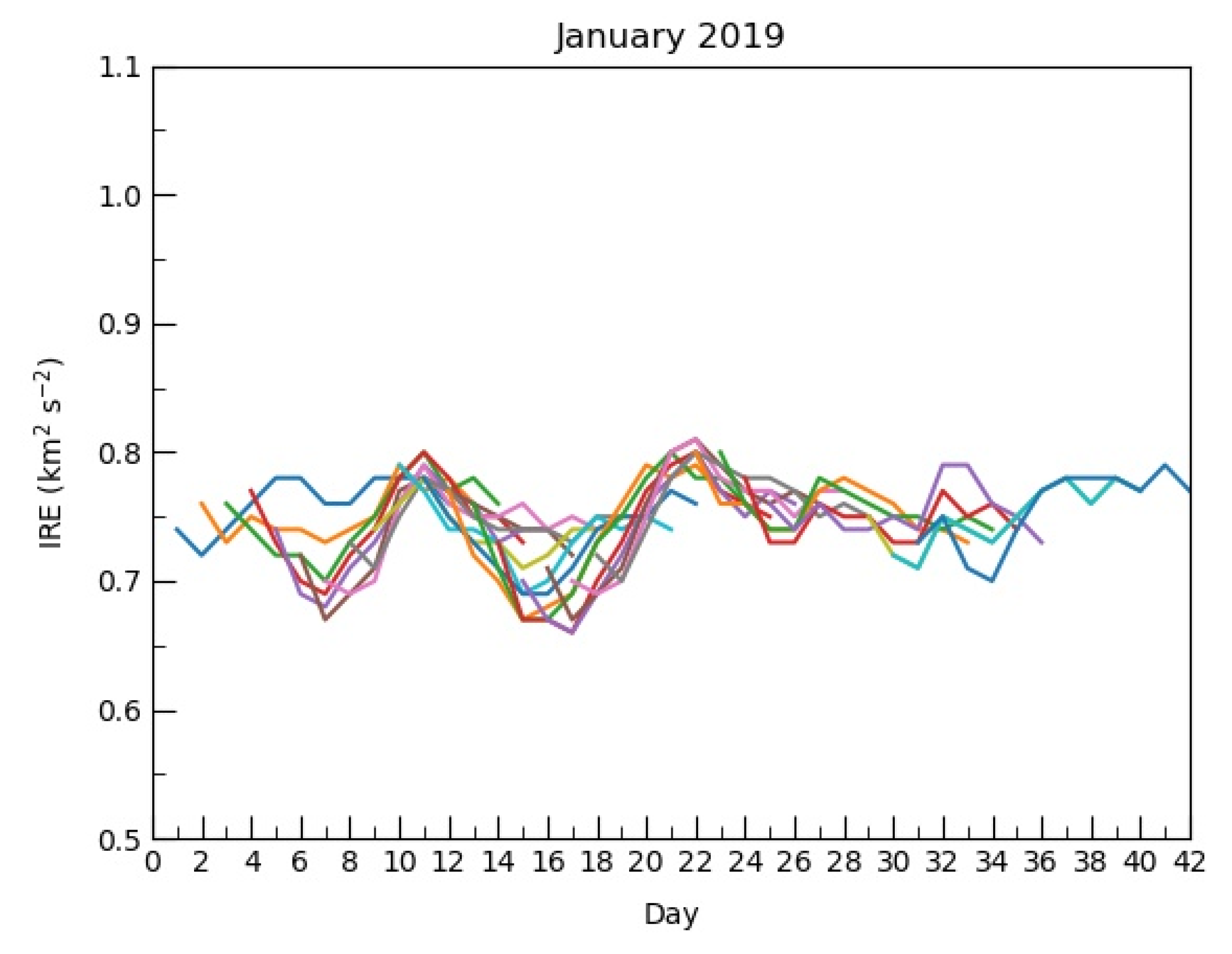
As stated in Section 2, the NAEFS ensembles were available out to 14 days. In order to simplify the analysis here, we examined the ensemble mean forecast IE from one to 10 days in order to determine whether the ensemble model could detect regime transition at this range. The strategy used here was similar to [37] in that the forecast evaluation began 10 days before the identified regime transition, and then examples were presented for 10, seven, four, and one day out from the identified observed IE maximum/regime transition. Given that some flow regimes persisted for less than 10 days, some of the associated 10 and seven-day IE forecasts overlap two IE maxima or regime transitions. Thus, this section will examine the 10 day mean ensemble NH IE forecast ‘plumes’ relative to individual regime transitions only. An example (Figure 3) of the daily NAEFS mean 10-day ensemble NH IE ‘plumes’ is shown for all of January 2019. Note, these generally identify the observed IE maxima in Figure 1. Additionally, an observed IE maximum occurred on 1 February and that also was identified by NAEFS ensemble mean forecast NH IE.

Initially, the mean ensemble IE 10-day forecasts were evaluated in order to determine whether or not the ensemble model forecast produced a local IE maximum and how close temporally this maximum was to the observed NH IE maximum. These results are shown in Figure 4 and

Table 2. The probability of detection (POD, 0.00–1.00), the miss rate (MISS, 0.00–1.00), false alarm rate (FAR, 0.00–1.00), mean over-forecast (positive)/under-forecast (negative) (MEAN–days), and standard deviation (STDEV–days) for the NAEFS mean ensemble IE forecasts. The latter two quantities are constructed from the data in Figure 4.

Forecast	POD	MISS	FAR	MEAN	STDEV
10-day	0.38	0.62	0.59	−1.5	1.4
7-day	0.85	0.15	0.12	+0.1	1.1
4-day	0.79	0.21	0.21	+1.0	1.4
1-day	0.90	0.10	0.10	+0.4	1.6

. In Figure 4 and Table 2, most model IE forecast maxima were predicted by the NAEFS ensemble mean within one day of actual maximum. This is confirmed by examining the mean forecast lag/lead shown in Table 2. The standard deviation for all these forecasts was between one and two days (1.4 days). Thus, here a ‘correct’ forecast for the IE maximum was counted within one day of the observed IE maximum.

The one-day forecast POD was the best at 0.90; however, the second-best POD was noted for the seven-day model forecasts (0.85). As expected, the POD decreased substantially after this and the 10-day forecasts performed the worst at 0.38. The miss rate (MISS) counted maxima that were either not forecast at all or forecast outside the one-day verification window, while the FAR was only the count of forecasts outside the one-day window. The 10-day forecasts were consistently under-forecast in the sense that the mean ensemble IE forecast maximum was 1.5 days too early. The other forecast categories projected the model IE maximum to occur too late. Only nine of the observed IE maxima were correctly forecast at 10 days. The seven-day forecasts were best in that the mean forecast IE maximum occurred in the model at seven days. For the one-day forecasts, only four mean ensemble IE forecasts occurred outside the +/− one day window. Three of these were forecast at day four or day five (counted as a MISS and FAR) and in one instance was not forecast in the entire 10 days (MISS).

Then using (4), the sensitivity index demonstrates that the one, four, and seven-day mean IE ensemble forecasts, respectively, successfully project signal above the noise, a result significant at p = 0.01, 0.1, and 0.05, respectively. Only the 10-day forecasts were not statistically significant. The forecast bias was calculated as the (POD + MISS)/(POD + FAR), and the bias was 1.0, 1.03, and 0.99 for the one, four, and seven-day forecasts, respectively, indicating little bias in these forecasts. Finally, if all the forecast performances are combined, the sensitivity index indicates significance at p = 0.10 (POD = 0.73 and FAR = 0.25).

3.3. IE Skill

The skill score (3) is a measure representing the value added for a particular forecast over some baseline or how close to perfection the forecast is from the baseline [49]. In order to examine the ability of the NAEFS mean ensemble model to capture the magnitude or value of the observed IE maximum, the skill scores and mean absolute error is shown in

Table 3. As in Table 2, except for the mean absolute error (forecast − observations = MAE), mean number of points for the forecast period (0.00–2.00), and skill score (0.00–1.00).

Forecast	MAE	Points	Skill
10-day	0.019	1.44	0.42
7-day	0.029	1.47	0.45
4-day	0.018	1.58	0.56
1-day	0.006	1.74	0.74
Climatology	0.064	1.03	0.00

. As expected, the one-day forecasts performed the best, while the skill deteriorated with forecast lead time out to seven days. There was little difference in the skill of the seven-day forecast of mean ensemble forecast IE versus the 10-day forecasts.

The work of [40] found that climatology was difficult to beat when considering the skill for forecasts of surface temperature anomalies in long-range forecasting, while it is well known that for short-range forecasts climatology is not difficult to beat. However, [40] also showed that the skill for forecasts of events that were two or more standard deviations above and below normal were better forecast using teleconnections. It was expected here that climatology would provide a reasonable baseline.

If a forecast evaluated as two (zero) points was considered a ‘hit’ (‘bust’), there were 10 (9) forecast hits (busts) for climatology out of the 34-ensemble mean IE forecast maxima. For the 10, seven, four, and one-day ensemble mean NH IE forecasts, 18, 20, 23, and 24 could be considered a ‘hit’, respectively. The busted forecast counts were four, four, four, and one were considered a bust respectively.

In summary, Section 2.2 established a quantitative measure for identifying local maxima for NH IE that previous studies in this group had only identified qualitatively. Moreover, this section demonstrated that the NAEFS ensemble identified a similar number of NH IE maxima from May 2018–April 2019 (34) to the mean annual occurrence of these maxima (30–35) found in a 30-year climatological study in [2]. Thus, the criteria established here likely is robust.

The NAEFS mean ensemble showed skill in projecting major changes in the large-scale NH flow as much as ten days in advance as identified using the NH IE diagnostic of [16] and used in this form or as a regional variant by this research group in many studies. The model performed more reliably at lesser lead times as expected. Using the skill score to evaluate the NAEFS ensemble model ability to anticipate the relative strength of the maximum showed that the skill scores were greater than 0.50 for the four and one-day forecasts with respect to climatology. Even at seven days, the skill score is nearly 0.50 and the number of forecasts counted as a “HIT” were consistent with the four and one-day forecasts. The POD results also demonstrated that the NAEFS ensemble model mean forecasts could identify the regime transitions above the noise at one, four, and seven days at statistically significant levels. Overall, this indicates that the NAEFS ensemble mean IE as calculated using the 500 hPa flow forecasts are reliable out to seven days, which is consistent with the time frame given for the reliability of other operational model forecasts of 500 hPa height fields as measured using their criterion for anomaly correlation [11].

4. NH IE as an Indicator of Regional Synoptic Changes

In this section, the efficacy of IE maxima to indicate NH flow regime changes and the relationship to changes in weather and climate of our region (Missouri, USA—see Figure 5A) is examined here. Four cases were chosen and the mean temperature and accumulated precipitation characteristics for the 10-day period before and after the observed IE maximum are given in Figure 5 and Figure 6 and

Table 4. The date of an observed NH IE maximum. Moreover, the major NH teleconnection indexes (PDO/NAO/AO), and the temperature (T °C) and precipitation (mm) character for Saint Louis, Missouri (MO) (STL), Columbia, MO (COU), Kansas City, MO (EAX), and Springfield, MO (SGF) for the ten days before and after the observed IE maximum. The temperature anomalies and the monthly standard deviation (σ) relative to the 1981–2010 means are also listed (see: [54]).

Date	Teleconnections		STL	COU	EAX	SGF
			T °C/mm
21 Aug 18	0.55/0.37/1.26	Before	26.2/32.5	25.9/27.4	24.8/65.5	25.6/70.4
		T °C anomaly	+0.1	+1.0	−0.5	−0.7
	−1.26/0.81/0.97	After	26.0/44.5	25.6/49.5	24. 8/35.1	24.7/75.2
			+0.7	+1.7	+0.7	+0.1
		Aug σ	1.7	1.8	1.9	1.7
23 Sep 18	−1.80/0.74/0.47	Before	25.7/1.3	24.6/29.0	23.8/7.9	24.1/3.3
			+5.0	+5.6	+4.4	+4.4
	−0.87/0.42/0.92	After	22.0/8.9	20.3/6.9	18.6/7.1	20.4/18.8
			+3.6	+3.6	+1.6	+2.9
		Sep σ	1.3	1.4	1.6	1.4
27 Oct 18	1.95/0.34/0.33	Before	10.6/11.7	10.5/6.9	12.6/1.8	12.2/11.9
			−3.3	−2.0	−0.1	−2.4
	0.04/0.74/−0.37	After	12.6/66.5	10.7/57.7	10.7/13.2	10.9/53.3
			−0.1	0.0	+0.3	−0.7
		Oct σ	1.4	1.4	1.3	1.3
14 Feb 19	−4.38/−0.21/0.95	Before	+0.2/67.8	−1.1/31.8	−3.2/17.0	+2.5/51.3
			−1.4	−1.6	−3.4	+0.3
	−3.55/−0.06/2.13	After	+1.1/21.6	−1.2/13.0	−4.0/37.3	+0.9/26.2
			−2.0	−3.1	−6.1	−2.8
		Feb σ	2.6	2.7	2.9	2.4

. Ten days was chosen since it is the length of the model forecast period and a flow regime transition occurred approximately every 10.7 days as shown in Section 3. Two cases (23 September 2018 and 14 February 2019) were chosen since they corresponded to strong changes in the weather across our region and these changes were well-forecast in the one to three-day (short-range) time period by the NAEFS ensemble mean. One case (21 August, 2018) was chosen such that the observed IE maximum was missed by the day-one mean ensemble model forecast (a maximum does not occur until day-six). The last case was a strong IE maximum case chosen completely at random (27 October, 2018). These cases are discussed in calendar order.

For the 10 days preceding the first case study (21 August), Figure 5A and Table 4 showed a relatively zonal 500 hPa ridge-trough configuration over northern North America (Figure 5A). The sea level pressure (SLP) map shows that the Midwest USA is dominated by a trough (Figure 6A). During the 10-day period following this transition, the 500 hPa flow showed a slightly more amplified pattern (Figure 5B) that was 180 degrees out of phase with the previous period as reflected by the strong change in the PNA index (Figure 5A,B, and Table 4). The SLP (Figure 6B) shows the Missouri region on the upstream side of high pressure. What was not clear immediately is why the model mean ensemble missed the IE maximum on day one. This should be the subject of a follow-up study.

The temperature and precipitation regime for the study region changed very little prior and following 21 August (Table 4). The temperature regime was very close to the normal for each city for this time of year (Table 4) and the temperature was generally less than one standard deviation from the normal temperature. Only one subtle change was noted in that precipitation was observed on six days of ten before the observed IE maximum and four days of ten following within the region. Additionally, 25.4–36.8 mm of precipitation would be expected across the state for the 10 days before and after 21 August [55]. The amount of precipitation before and after the transition date could be described as typical except for southwest Missouri (SGF), which received approximately double the typical amount of precipitation. No blocking was observed in the Pacific or Atlantic sectors during this period of time and [40,56] demonstrated the correlation of the large-scale flow regime upstream and downstream of the central USA.

The second case (23 September, 2018) occurred during a very warm September across the region, and a strong cold front passed through Missouri close to this date. The jet stream before this date was located far to the north (Figure 5C). Before the IE maximum, a trough was located over western North America (Figure 5C) at 500 hPa, but over the middle of the continent in the ten days following (Figure 5D). The SLP fields (Figure 6C,D) shows that the study region was downstream of a weak trough and generally northeasterly flow [55] before the IE maximum, but with more of a southerly flow component following the maximum. Table 4 shows that the PNA and AO became more positive and the NAO more negative following 23 September. Before 23 September, 2018, the temperatures across the region were more than three (and even four) standard deviations greater than normal.

This flow regime prior to 23 September was also quite dry and measurable precipitation was noted regionwide for only two of the ten days. It would be expected that 26.4–39.1 mm of precipitation would have occurred during the ten-day period prior; however, conditions were generally dry across the state (Table 4). Following the large-scale flow regime change (Table 4), temperatures decreased significantly (as much as 5 °C). The days following 23 September were still relatively dry (Table 4—also two days of measurable precipitation regionally) and warm, but only one to just under three standard deviations above normal. During the ten-day period following the change in flow regime, blocking was noted over the eastern Pacific [57]. This correlates often with cooler conditions over the central USA [56].

The third case (27 October, 2018) was associated with cooler conditions regionally 10-days prior to the observed IE maximum, but then warmer conditions during the 10 days following the maximum. The large-scale flow for the period prior to the IE maximum (Figure 5E) was characterized as an amplified 500 hPa ridge-trough pattern, and high pressure dominated the study region in the SLP field (Figure 6E). Table 4 showed a strongly more negative PNA index, a more negative AO index, and a more positive NAO. Following the 27 October period, the large-scale flow showed a trough over the middle North America, but zonal flow upstream (Figure 5F). In the SLP map, the middle of the United States was dominated by a trough (Figure 6F).

For the 10-days prior to the IE maximum (Table 4), the temperatures were generally about one to two standard deviations below normal regionally except for northwest Missouri. Following the IE maximum and the large-scale flow regime change temperatures were close to normal across the state. The biggest change was in the precipitation characteristics. Conditions before the observed IE maximum were dry (Table 4), and regionally, measurable precipitation occurred during three days. For a ten-day period in October, 26.7–30.0 mm of precipitation would be expected across the state [55]. Following the IE maximum, conditions were much wetter except for the northwest part of the state (Table 4) and precipitation occurred on six of the ten days. Additionally, blocking occurred over the eastern Pacific during mid-October [57], which could be linked to the cooler conditions prior to 27 October 2018.

The last case study was associated with a strong IE maximum observed in mid-February 2019. During the 10-days before the 14 February IE maximum, there was a 500 hPa trough located over the eastern Pacific and western North America (Figure 5G). The SLP map (Figure 6G) showed the study region was between a strong high-pressure region to the northwest and high pressure to the southeast. Table 4 demonstrates that the period was within the range of normal (generally less than one standard deviation below normal for three of the cities, except for Kansas City, which was about one sigma below normal. The 10-day period was comparatively wet, but little snow was observed across the region (not shown here—see [52]). This period was also much wetter than normal as the state experiences 12.4 to 21.3 mm of precipitation in early February [55]. Additionally, this case was the best anticipated by the NAEFS mean ensemble forecast IE as the 10-day, 4-day forecast each anticipated the observed IE maximum, while the seven-day forecast anticipated the IE maximum on day-eight.

For the 10-day period following the observed IE maximum (Figure 5H), the 500 hPa trough was located further east over North America and Table 4 indicates all three teleconnection indexes became more positive, especially the AO. The SLP map (Figure 6H) shows that the study region was under the influence of the high pressure to the north to a greater extent even though the high itself had weakened. Moreover, the temperature regime cooled considerably as three of the cities were nearly or more than one-standard deviation cooler than normal and northwest Missouri (EAX) was more than two standard deviations below normal. The precipitation regime was a little drier but over the northern part of the state, but snow was observed ranging from 6 cm in the eastern part of the region to 20 cm or more in the western part of the region [55]. Lastly, two mid-February blocking events [55], one over the east Pacific and one over the eastern Atlantic were both partly responsible for bringing colder conditions over the central USA.

In summary, three of these case studies demonstrated that relatively large changes in the temperature and precipitation character of the local weather can reasonably be anticipated in association with the observed maxima in NH IE. This result combined with Section 3 demonstrates that these changes can be anticipated in the long-range of synoptic-scale forecasting (seven to 10 days). In fact, the mid-February change was anticipated more than seven days ahead in real-time following the model guidance during the performance of this research. In only one of these four cases did the NAEFS ensemble miss the large-scale NH flow regime change in the short range. Moreover, there was not a very strong change in regional temperature and precipitation regimes as associated with this missed short-term observed IE maximum.

5. Summary and Conclusions

In this study, the ability of the NAEFS ensemble model to project the occurrence of observed IE maxima in the large-scale NH flow was tested using traditional measures of skill as well as signal detection theory. The latter is typically used for smaller scale-phenomena, but was useful in anticipating the timing of the model forecast of observed IE maxima. The model ensemble mean 500 hPa height fields were used, and the IE diagnostic derived in [16] and employed by [2] in this research group to identify large-scale flow regime transitions or blocking. The model data had relatively fine resolution (1° × 1° latitude–longitude). The observed IE was calculated using the NCEP reanalyses 500 hPa height fields available on a grid with resolution of 2.5° latitude/longitude.

Once these IE maxima were identified using a quantitative criterion and confirmed by examining the major NH teleconnection indexes, the timing and strength of the model forecast maxima were analyzed and summarized by presenting the results for the ten, seven, four, and one day model forecasts. The development of this quantitative criterion for identifying IE maxima was not done by other work previously published by this research group. Then four case studies were examined in order to determine whether these observed IE maxima were associated with strong changes in regional (central USA) temperature and precipitation regimes. These temperature and precipitation data were obtained via the National Weather Service [55] archives. The following results were obtained.

Using signal detection methods, the NAEFS model ensemble generally anticipated an observed IE maximum within one day of its occurrence for forecasts out to seven days. The mean model forecast was approximately one day late, but at 10 days, the mean model forecast IE maximum was about 1.5 days early on average. Signal detection theory demonstrated that the model could project these observed maxima seven days prior to the occurrence and that the signal was identifiable above noise at p = 0.10 or greater.

Using traditional skill score, the NAEFS mean ensemble model forecast IE maxima showed skill well above that of climatology for the entire 10 day forecast period, although skill did decrease with greater lead time. Thus, using signal detection methods and skill score, the prediction of IE maximum occurrence and strength was reliable out to at least seven days. This is at least at the end of the current range of operational forecast model ability to predict 500 hPa height fields.

Lastly, the observed IE maxima, associated with large-scale flow regime changes, could be associated often with changes in the regional temperature and precipitation regimes and character as identified using four case studies. Thus, the results of Section 3 and Section 4 taken together indicated that the integrated enstrophy diagnostic of [16] has value and skill in projecting changes in the large-scale and regional scale weather for long-range synoptic-scale forecasts.

References

1. Li, Y.C. Linear hydrodynamic stability. N. Am. Math. Soc. 2018, 65, 1255–1259. [Google Scholar] [CrossRef]
2. Jensen, A.D.; Akperov, M.G.; Mokhov, I.I.; Lupo, A.R.; Fengpeng, S. The dynamic character of northern hemisphere flow regimes in a near-term climate change projection. Atmosphere 2018, 8, 27. [Google Scholar] [CrossRef] [Green Version]
3. Namias, J. The great Pacific anticyclone of the winter 1948–50: A case study in the evolution of climatic anomalies. J. Meteorol. 1951, 8, 251–261. [Google Scholar] [CrossRef]
4. Lorenz, E.N. Seasonal and irregular variations of the Northern Hemisphere sea-level pressure profile. J. Meteorol. 1951, 8, 52–59. [Google Scholar] [CrossRef] [Green Version]
5. Wallace, J.M.; Gutzler, D.S. Teleconnections in the Geopotential Height Field during the Northern Hemisphere Winter. Mon. Weather Rev. 1981, 109, 784–812. [Google Scholar] [CrossRef]
6. Birk, K.; Lupo, A.R.; Guinan, P.; Barbieri, C.E. The interannual variability of Midwestern temperatures and precipitation as related to the ENSO and PDO. Atmósfera 2010, 23, 95–128. [Google Scholar]
7. Keables, M.J. Spatial variability of mid-tropospheric circulation patterns and associated surface climate in the United States during ENSO winters. Phys. Geogr. 1992, 13, 331–348. [Google Scholar] [CrossRef]
8. American Meteorological Society—Weather Analysis and Forecasting. Available online: https://www.ametsoc.org/ams/index.cfm/about-ams/ams-statements/statements-of-the-ams-in-force/weather-analysis-and-forecasting/ (accessed on 14 July 2020).
9. Lorenz, E.N. The predictability of hydrodynamic flow. Proc. N. Y. Acad. Sci. 1963, 25, 409–432. [Google Scholar]
10. Lorenz, E.N. A study of the predictability of a 28-variable atmospheric model. Tellus 1965, 17, 321–333. [Google Scholar] [CrossRef] [Green Version]
11. European Centre for Medium-Range Weather Forecast. Annual Report 2017. European Centre for Medium-Range Weather Forecast; European Centre for Medium-Range Weather Forecast: Reading, UK, 2018; pp. 1–40. [Google Scholar]
12. Krishnamurthy, V. Predictability of Weather and Climate. Earth Space Sci. 2019, 6, 1043–1056. [Google Scholar] [CrossRef] [Green Version]
13. Lupo, A.R.; Li, Y.C.; Feng, Z.C.; Fox, N.I.; Rabinowitz, J.L.; Simpson, M.L. Sensitive versus rough dependence under initial conditions in atmospheric flow regimes. Atmosphere 2016, 7, 157. [Google Scholar] [CrossRef] [Green Version]
14. Deloncle, A.; Berk, R.; D’Andrea, F.; Ghil, M. Weather regime prediction using statistical learning. J. Atmos. Sci. 2007, 64, 1619–1635. [Google Scholar] [CrossRef] [Green Version]
15. Miller, D.E.; Wang, Z.; Trapp, R.J.; Harnos, D.S. Hybrid prediction of weekly tornado activity out to Week 3: Utilizing weather regimes. Geophys. Res. Lett. 2020, 47, e2020GL087253. [Google Scholar] [CrossRef]
16. Jensen, A.D.; Lupo, A.R.; Mokhov, I.I.; Akperov, M.G.; Reynolds, D.D. Integrated regional enstrophy and Block Intensity as a measure of Kolmogorov Entropy. Atmosphere 2017, 8, 237. [Google Scholar] [CrossRef] [Green Version]
17. Dymnikov, V.P.; Kazantsev, Y.V.; Kharin, V.V. Information entropy and local Lyapunov exponents of barotropic atmospheric circulation. Izv. Atmos. Ocean. Phys. 1992, 28, 425–432. [Google Scholar]
18. Lupo, A.R.; Mokhov, I.I.; Dostoglou, S.; Kunz, A.R.; Burkhardt, J.P. Assessment of the impact of the planetary scale on the decay of blocking and the use of phase diagrams and enstrophy as a diagnostic. Izv. Atmos. Ocean. Phys. 2007, 43, 45–51. [Google Scholar] [CrossRef]
19. Hussain, A.; Lupo, A.R. Scale and stability analysis of blocking events from 2002 to 2004: A case study of an unusually persistent blocking event leading to a heat wave in the Gulf of Alaska during August 2004. Adv. Meteor. 2010, 610263. [Google Scholar] [CrossRef]
20. Jensen, A.D.; Lupo, A.R. The role of deformation and other quantities in an equation for enstrophy as applied to atmospheric blocking. Dyn. Atmos. Ocean. 2014, 66, 151–159. [Google Scholar] [CrossRef]
21. Athar, H.; Lupo, A.R.; Strong, C.; Dostoglou, S. A Diagnostic Study on Atmospheric Blocking Using Lyapunov Exponents over a 50-Year Period. Available online: https://ams.confex.com/ams/87ANNUAL/techprogram/paper_116915.htm (accessed on 29 May 2020).
22. Jensen, A.D. A dynamic analysis of a record breaking winter season blocking event. Adv. Meteorol. 2015, 2015, 634896. [Google Scholar] [CrossRef] [Green Version]
23. Nakamura, N.; Huang, C.S.Y. Atmospheric blocking as a traffic jam in the jet stream. Science 2018, 361, 42–47. [Google Scholar] [CrossRef]
24. Luo, D.; Zhang, W.; Zhong, L.; Dai, A. A Nonlinear theory of atmospheric blocking: A potential vorticity gradient view. J. Atmos. Sci. 2019, 76, 2399–2427. [Google Scholar] [CrossRef]
25. Lucarini, V.; Gritsun, A. A new mathematical framework for atmospheric blocking events. Clim. Dyn. 2020, 54, 575–598. [Google Scholar] [CrossRef] [Green Version]
26. Lupo, A.R.; Smith, P.J. Climatological features of blocking anticyclones in the Northern Hemisphere. Tellus Ser. A 1995, 47, 439–456. [Google Scholar] [CrossRef] [Green Version]
27. Lupo, A.R.; Smith, P.J. Planetary and synoptic-scale interactions during the life cycle of a mid-latitude blocking anticyclone over the North Atlantic. Tellus Spec. Issue Life Cycles Extratropical Cyclones 1995, 47, 575–596. [Google Scholar]
28. Burkhardt, J.P.; Lupo, A.R. The planetary and synoptic-scale interactions in a Southeast Pacific blocking episode using PV diagnostics. J. Atmos. Sci. 2005, 62, 1901–1916. [Google Scholar] [CrossRef] [Green Version]
29. Lupo, A.R.; Smith, P.J. The interactions between a mid-latitude blocking anticyclone and synoptic-scale cyclones occurring during the northern hemisphere summer season. Mon. Weather Rev. 1998, 126, 503–515. [Google Scholar] [CrossRef] [Green Version]
30. Lupo, A.R.; Mokhov, I.I.; Akperov, M.G.; Cherokulsky, A.V.; Athar, H. A dynamic analysis of the role of the planetary and synoptic scale in the summer of 2010 blocking episodes over the European part of Russia. Adv. Meteorol. 2012, 2012, 584257. [Google Scholar] [CrossRef] [Green Version]
31. Kalnay-Rivas, E.; Merkine, L.O. A simple mechanism for blocking. J. Atmos. Sci. 1981, 38, 2077–2091. [Google Scholar] [CrossRef]
32. Mullen, S.L. Transient eddy forcing and blocking flows. J. Atmos. Sci. 1987, 44, 3–22. [Google Scholar] [CrossRef]
33. Tsou, C.H.; Smith, P.J. The role of synoptic/planetary-scale interactions during the development of a blocking anticyclone. Tellus 1990, 42, 174–193. [Google Scholar] [CrossRef]
34. Haines, K.; Holland, A.J. Vacillation cycles and blocking in a channel. Q. J. Roy Meteor Soc. 1998, 124, 873–895. [Google Scholar] [CrossRef]
35. Colucci, S.J.; Baumhefner, D.P. Numerical prediction of the onset of blocking: A case study with forecast ensembles. Mon. Weather Rev. 1998, 126, 773–784. [Google Scholar] [CrossRef]
36. Tilly, D.E.; Lupo, A.R.; Melick, C.J.; Market, P.S. Calculated height tendencies in two southern hemisphere blocking and cyclone events: The contribution of diabatic heating to block intensification. Mon. Weather Rev. 2008, 136, 3568–3578. [Google Scholar] [CrossRef] [Green Version]
37. Reynolds, D.D.; Lupo, A.R.; Jensen, A.D.; Market, P.S. The predictability of northern hemispheric blocking using an ensemble mean forecast system. Open Atmos. Sci. J. 2019, 13, 3–17. [Google Scholar] [CrossRef]
38. Matsueda, M. Predictability of euro-russian blocking in summer of 2010. Geophys. Res. Lett. 2011, 38, L06801. [Google Scholar] [CrossRef]
39. Jensen, A.D.; Lupo, A.R. Using enstrophy advection as a diagnostic to identify blocking-regime transition. Q. J. R. Meteorol. Soc. 2014, 140, 1677–1683. [Google Scholar] [CrossRef]
40. Renken, J.S.; Herman, J.J.; Bradshaw, T.R.; Market, P.S.; Lupo, A.R. The utility of the Bering Sea and East Asia rules in long-range forecasting. Adv. Meteorol. 2017, 2017, 1765428. [Google Scholar] [CrossRef]
41. NCEP/NCAR Reanalyses Project. Available online: http://www.esrl.noaa.gov/psd/data/reanalysis/reanalysis.shtml (accessed on 6 May 2019).
42. Climate Diagnostic Bulletin. Available online: https://www.cpc.ncep.noaa.gov/products/CDB/CDB_Archive_pdf/pdf_CDB_archive.shtml (accessed on 13 May 2019).
43. Climate Prediction Center: Weather and Climate Linkages. Available online: https://www.cpc.ncep.noaa.gov/products/precip/CWlink/daily_ao_index/teleconnections.shtml (accessed on 12 May 2020).
44. Global Ensemble Forecast System (GEFS) and Northern American Ensemble Forecast System (NAEFS). Available online: https://www.emc.ncep.noaa.gov/gmb/yzhu/gif/pub/GEFSUserGuide_V1.0.pdf (accessed on 23 April 2019).
45. North American Ensemble Forecast System. Available online: https://www.emc.ncep.noaa.gov/gmb/ens/NAEFS.html (accessed on 23 April 2019).
46. North American Ensemble Forecast System (NAEFS). Available online: https://weather.gc.ca/ensemble/naefs/index_e.html (accessed on 23 April 2019).
47. Oseledets, V.L. A multiplicative ergodic theorem. Lyapunov characteristic numbers for dynamical systems. Trans. Mosc. Math. Soc. 1968, 19, 179. [Google Scholar]
48. Ekmann, J.P.; Ruelle, D. Ergodic theory of chaos. Rev. Mod. Phys. 1985, 57, 617–656. [Google Scholar] [CrossRef]
49. Lupo, A.R.; Market, P.S. The verification of weather forecasts in Central Missouri and seasonal variations in forecast accuracy. Weather Forecast. 2002, 8, 891–897. [Google Scholar] [CrossRef]
50. Wickens, T.D. Elementary Signal Detection Theory; Oxford University Press: Oxford, UK, 2001. [Google Scholar]
51. Macmillan, N.; Creelman, C. Detection Theory: A Users Guide; Taylor and Francis: Abingdon, UK, 2004; Volume 512. [Google Scholar]
52. Neter, J.; Wasserman, W.; Whitmore, G.A. Applied Statistics, 3rd ed.; Allyn and Bacon: Boston, MA, USA, 1988. [Google Scholar]
53. Balkissoon, S.S.; Bongard, J.T.; Cain, T.; Candela, D.M.; Clay, C.; Efe, B.; Ji, Q.; Klaus, E.M.; Korner, A.P.; Mitchell, K.; et al. Hurricane florence makes landfall in the Southeast USA: Sensitive dependence on initial conditions, parameterizations, and integrated enstrophy. Atmos. Clim. Sci. 2020, 10, 98159. [Google Scholar] [CrossRef] [Green Version]
54. National Climatic Data Center (NCDC) USA Website. 2020. Available online: https://www.ncdc.noaa.gov/cag/city/time-series/ (accessed on 7 August 2020).
55. National Weather Service (NWS). 2020. Available online: http://www.weather.gov (accessed on 7 August 2020).
56. Nunes, M.J.; Lupo, A.R.; Lebedeva, M.G.; Chendev, Y.G.; Solovyov, A.B. The occurrence of extreme monthly temperatures and precipitation in two global regions. Pap. Appl. Geogr. 2017, 6. [Google Scholar] [CrossRef] [Green Version]
57. The University of Missouri Blocking Archive. 2020. Available online: https://weather.missouri.edu/gcc (accessed on 3 June 2020).
Figure 1. The (a) observed Northern Hemisphere (NH) Integrated enstrophy (IE) time series (km2 s−2—solid red line) and (b) 24 h change in NH IE (km2 s−2)—red bars) for January 2019. The ordinate is (a) IE or (b) the change in IE. The abscissa is day of the month.
Atmosphere 11 00915 g001
Figure 2. As in Figure 1, except for the time series of the Pacific North American Index (blue, solid), North Atlantic Oscillation (orange, solid), and Arctic Oscillation (gray, solid).
Atmosphere 11 00915 g002
Figure 3. The daily North American Ensemble Forecast System (NAEFS) ensemble mean 10-day forecasts of NH IE for each day in January 2019. Each day (plume) is represented by a different color (e.g., 1 January, 2 January, 3 January, 4 January, 5 January, 6 January, 7 January, 8 January are represented by blue, orange, green, red, purple, brown, lavender, light blue, respectively) until 9 January when the color scheme repeats.
Atmosphere 11 00915 g003
Figure 4. The (a) ten, (b) seven, (c) four and (d) one day NAEFS ensemble mean IE forecast prior to an observed IE maximum associated with regime transition. The ordinate is the number of model forecasts and the abscissa is the number of days prior (−) or following (+) the model forecast local IE maximum was from the observed IE maximum.
Atmosphere 11 00915 g004aAtmosphere 11 00915 g004b
Figure 5. The 500 hPa height field for North America for the 10 days prior to an observed IE maximum; (A) 21 August, 2018, (C) 23 September, 2018, (E) 27 October, 2018, and (G) 14 February, 2019, and the 10 days following the IE maximum date for (B) case one, (D) case two, (F) case three, and (H) case four. The arrow in Figure 5A shows the location of Missouri, USA.
Atmosphere 11 00915 g005
Figure 6. The Sea Level Pressure (hPa) for North America for the 10 days prior to an observed IE maximum; (A) 21 August, 2018, (C) 23 September, 2018, (E) 27 October, 2018, and (G) 14 February, 2019, and the 10 days following the IE maximum date for (B) case one, (D) case two, (F) case three, and (H) case four. The contour interval is 2 hPa. The H and L are sea level pressure centers, while the dashed (solid) lines are troughs (ridges) of low (high) pressure regions.
Atmosphere 11 00915 g006aAtmosphere 11 00915 g006b