Evaluation of Rainfall Forecasts by Three Mesoscale Models during the Mei-yu Season of 2008 in Taiwan. Part II: Development of an Object-Oriented Method

Abstract

This study describes a recently developed object-oriented method suitable for Taiwan for the purpose to verify quantitative precipitation forecasts (QPFs) produced by mesoscale models as a complement to the traditional approaches in existence. Using blended data from the rain-gauge network in Taiwan and the Tropical Rainfall Measuring Mission (TRMM) as the observation, the method developed herein is applied to twice-daily 0–48 h QPFs produced by the Cloud-Resolving Storm Simulator (CReSS) during the South-West Monsoon Experiment (SoWMEX) in May–June 2008. In this method, rainfall objects are identified through a procedure that includes smoothing and thresholding. Various attribute parameters and the characteristics of observed and forecast rain-area objects are then compared and discussed. Both the observed and the QPF frequency distributions of rain-area objects with respect to total water production, object size, and rainfall are similar to chi-distribution, with highest frequency at smaller values and decreased frequencies toward greater values. The model tends to produce heavier rainfall than observation, while the latter exhibits a higher percentage of larger objects with weaker rainfall intensity. The distributions of shape-related attributes are similar between QPF and observed rainfall objects, with more northeast–southwest oriented and fewer northwest–southeast oriented objects. Both observed and modeled object centroid locations have relative maxima over the terrain of Taiwan, indicating reasonable response to the topography. The above results are consistent with previous studies.

1. Introduction

Quantitative precipitation forecast (QPF) verification is a critical component in the development and use of forecasting systems [1,2]. It plays a crucial role in monitoring the quality of forecasts and to identify differences among forecasts made by different models or forecasters. The widely used traditional approaches, like the threat score (TS), equitable threat score (ETS) [3], bias score (BS), probability of detection (POD), false alarm ratio (FAR), etc. [4,5,6,7,8], are categorical statistics of the “measure-oriented” approach. Such measures have the advantages of reducing the vast amount of information from a set of forecasts and observations into a few single values and are thus easy to apply [9]. For the 12-h QPFs at the range of 12–36 h by the Pennsylvania State University National Center for Atmospheric Research (PSU-NCAR) fifth-generation mesoscale model (MM5) and the Weather Research and Forecasting (WRF) model for the Mei-yu season in Taiwan, for example, the averaged TS at low thresholds is about 0.2–0.25 [7,8] and lower than the forecast skill in the cold season at mid-latitudes [10] and also the typhoon season in Taiwan [11]. Today, forecasting approaches have become more complex due to the increase in the requirement of applicability at the finer scale.

As the model resolution increases, the traditional approaches for the verification of spatial forecasts like the QPFs, which tend to vary greatly in space and time, become less and less effective, at least in certain aspects. Some QPF verification methods, known as continuous statistics, employ the relationship between forecasts and observations typically for long-term periods [6], such as the absolute error, relative error, root mean squared error (RMSE), and correlation coefficient, are also very common [12,13]. While the above statistics of measure-oriented approach can provide measures to monitor system performance over time, they are typically inadequate to yield or derive specific information regarding the ways in which the forecasts went wrong or did well. Likewise, for categorical statistics like ETS, BS, and POD, the more detailed information about model behaviors is often hidden within the overall score results and faded. Moreover, due to issues like the “double penalty”, the point-to-point requirement in space and time between the observation, and QPFs make the above continuous and categorical statistics ineffective in model evaluation [14,15,16] and even more so as the resolution of numerical models increases [17,18,19].

On the other hand, subjective (eyeball) verification is usually quite informative with details and is capable to provide an overall understanding about model performances [20,21,22,23,24]. In either individual events or long-term averages, the patterns and characteristics of rainfall, like its location, areal extent and shape, peak amount, overall mean value, and even the spatial and temporal variabilities can be appropriately examined and compared with the observed patterns with subjective evaluation [20]. Due to its reliability for accurate interpretation of results, subjective methods are often necessary to complement other objective methods for QPF verification, as forecasts provide more details and structures in the rainfall field with the increase in model resolution [17,19,25,26,27,28]. However, in spite of being informative about the forecast errors in QPFs, subjective verification methods have a major drawback of being only qualitative and not quantitative and may be viewed as not objective enough to quantify the forecast errors.

Obviously, accurate QPFs in the location, spatial patterns, and structures of rainfall are essential for various aspects of applications like hydrology and climate change, etc. It has been noted that the amounts and spatial variability of rainfall have a major impact on the accuracy of both short-term precipitation and climate change forecasts [29]. In hydrological modelling, an accurate description of the spatial heterogeneity of precipitation, in terms of both pattern and location, is also important [30]. Presently, the categorical measures based on the 2 × 2 contingency table are probably the most widely used approach among all verification methods for QPFs [6,31]. Although they are more useful for rainfall caused by systems at larger scale, careful attention is needed to avoid the issue of double penalty on models that are capable of predicting the event but not at the correct location and time compared to those that cannot predict the event at all [32]. In view of the above problems of traditional verification methods and the lack of information in certain aspects, the more advanced countries like the United States and those in Europe have started to develop and use object-oriented methods for QPF verification [19,25,33,34,35,36,37] in a way similar to the methods used to verify the forecasts in location (track), intensity, and size of tropical cyclones for decades. Ebert and McBride [15] were among the first to explore and use an entity-based method to identify contiguous rainfall areas as a mean to verify rainfall forecasts. Hence, with the long history of object-based methods, the development of such a method suitable for Taiwan and its application seem appropriate at the present time, as carried out herein for the first time in Taiwan.

The development process largely follows the ideas of Davis et al. [19,25]. However, some adjustments and modifications are necessary in order to be applicable to the Taiwan region. The available methods already developed (such as Davis et al. [19,25] for the continental US) are designed for rainfall events from propagating systems such as mesoscale convective systems (MCSs), frontal systems, and extratropical cyclones in mid-latitudes. In Taiwan (which is a subtropical island surrounded by sea), while migratory rainfall systems are also often present, intense rainfall events at the local scale can also develop and are tied to the steep topography, as those in the Mei-yu season (May–June) in early summer. Moreover, the verification domain can also be much smaller due to the lack of sufficient rainfall data over the surrounding oceans. Thus, given the conditions of Taiwan with its complex and steep terrain, lack of in-situ data at sea, and localized precipitation systems, it is necessary to develop a non-traditional assessment method like the one presented in this study. Such a new generation of object-oriented method also represents an important step to fill the gaps of traditional methods in order to better understand the performance of model QPFs from all angles and eventually to improve the forecast ability of mesoscale models.

Object-based verification is especially relevant given the push toward higher-resolution forecasts and forecast verification of the phenomena that are highly localized and episodic, like convective rainfall [19,25]. The data period considered is the Mei-yu season of 2008 during the South-West Monsoon Experiment (SoWMEX) in Taiwan [38]. The remaining part of the present article is organized as follows. Section 2 describes the data. The development and application of the verification method are then discussed separately in Section 3 and Section 4, respectively. Discussion and conclusions are presented in Section 5.

2. Data

2.1. Observation Data

Owing to the high frequency of heavy rainfall in the Mei-yu season in Taiwan and easy access to data, the field phase of the SoWMEX experiment (15 May to 30 June 2008; Jou et al. [38]) was chosen as the target period in the present work. The details of the data are given below.

Central Weather Bureau (CWB) rainfall data: In this study, gauge data from the dense network of the Automatic Rainfall and Meteorological Telemetric System (ARMTS, [39,40]) are used (Figure 1 in Paul et al. [24]). Established and operated by the CWB, the ARMTS network includes 386 rain-gauge stations in 2008. The details of the data are described in Paul et al. [24] (hereafter, Part I), and thus, only necessary information is given here.

The Tropical Rainfall Measuring Mission (TRMM) gridded data from National Aeronautics and Space Administration (NASA) are used over the oceans and adjacent areas around Taiwan, where the CWB gauge data are unavailable. Provided by TRMM Multi-Satellite Precipitation Analysis (TMPA), this dataset (3B42) has a resolution of 0.25° × 0.25° every 3 h and employs a calibration-based sequential scheme to combine precipitation estimates from multiple satellites with gauge analyses at feasible locations (Huffman et al. [41]). The readers are referred to Part I for details [24].

The CWB gauge data and TRMM data are combined by means of the Cressman method [42], which is an objective analysis scheme to interpolate data onto grid points using a weighting function inversely proportional to distance. Here, the objective analysis is performed on the Cloud-Resolving Storm Simulator (CReSS) grid (to be described below) to merge ARMTS and TRMM data at 3-h intervals (also Paul et al. [24]). To better preserve the high resolution of ARMTS data, four rounds of analysis with an increasingly larger radius of influence (7.5, 15, 30, and 60 km, respectively) are used in the Cressman scheme (with higher priority in earlier rounds) for grid points over Taiwan. For those over ocean, on the other hand, only the four closest TRMM data points (0.25° apart) are used for interpolation in a single round.

2.2. Model Data

As mentioned, a cloud-resolving model, CReSS (version 2.2), developed by Nagoya University in Nagoya, Japan [43,44], is used in this study. The horizontal grid spacing is 3.5 km. The total grid points are 330 × 280, covering an area of 19–28° N, 113.5°–124.5° E (cf. Figure 1) with 40 vertical levels, are accommodated in a single domain without nesting. The model configuration and major physical options are given in

Table 1. Summary of configurations, initial and boundary conditions (ICs/BCs), and major physical options used in the CReSS model (version 2.2) for routine forecasts during the Mei-yu season (15 May–30 June) in 2008. In Taiwan, 00:00 UTC = 08:00 LST.

Model	CReSS (version 2.2)
Grid dimension (x, y, z)	330 × 280 × 40
Grid spacing (km)	3.5 × 3.5 × 0.5 (stretched over 0.1–0.663 km in vertical)
Domain size (km)	1155 × 980 × 20 (centered at 23.5° N, 119.0° E)
Projection	Lambert conformal (120° E, secant at 10° and 40° N)
IC/BCs	NCEP GFS analyses/forecasts (1° × 1°, 26 levels, every 3 h)
Topography and SST	Real at (1/120)° and NCEP analyses at 1° × 1°
Initial times (daily)	0000, 1200, and 1800 UTC (0800, 2000, and 0200 LST)
Forecast length	48 h
Output frequency	Every 15 min.
Cloud microphysics	Bulk cold-rain scheme (six species)
Planetary boundary layer	1.5-order closure with turbulent kinetic energy prediction
parameterization
Surface processes	Energy/momentum fluxes and shortwave/longwave radiation
Substrate soil model	41 levels, every 5 cm to 2-m deep

. The 0–48 h QPFs (summed to 3-h intervals) provided twice a day (from model runs initialized at 00:00 and 12:00 UTC) are considered here.

3. Development and Methodology

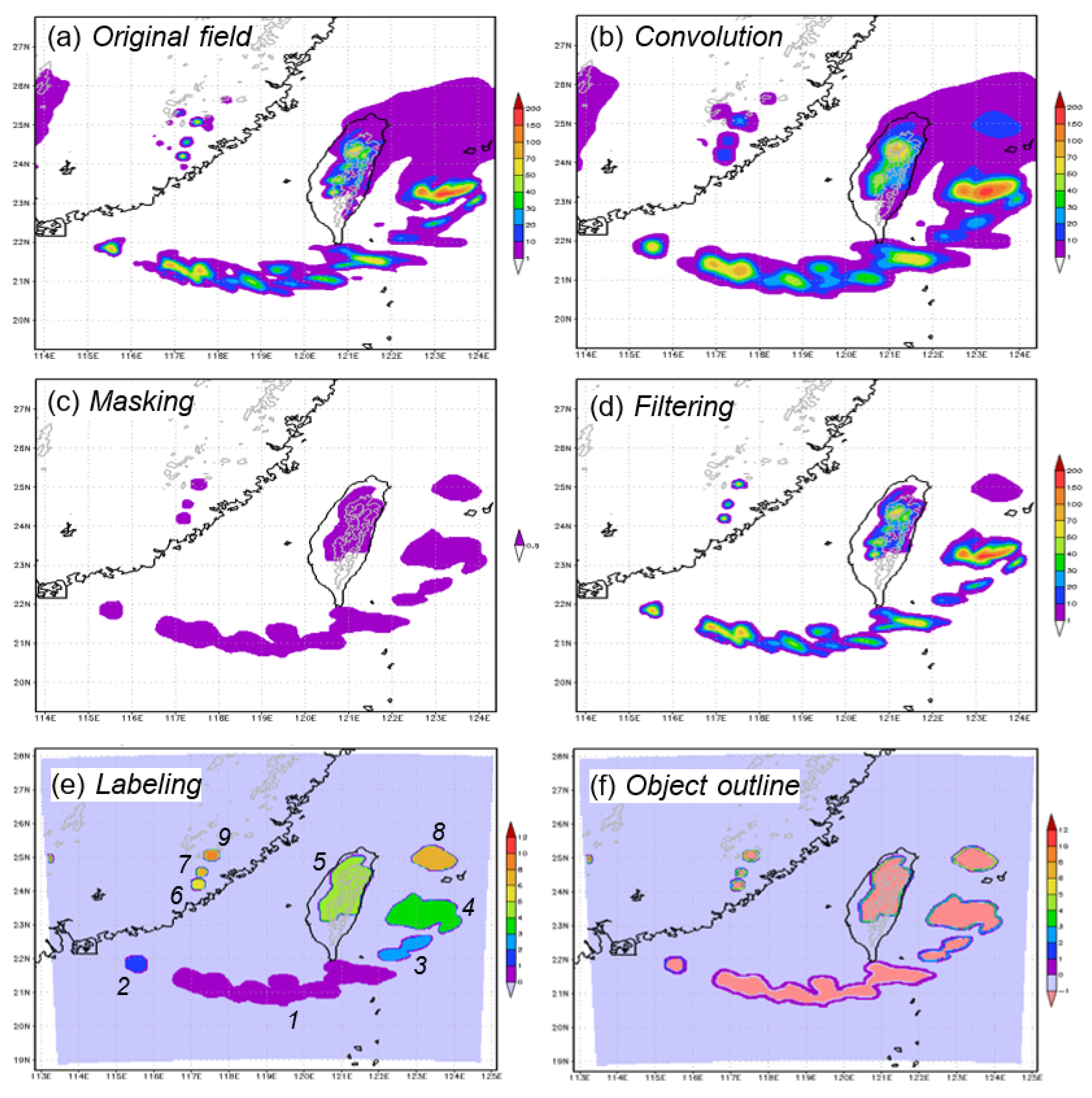
3.1. Identification of Mesoscale Rainfall Objects

In essence, object-based verification approaches compare the properties of observed and forecast objects, where the objects are in general precipitation areas determined using rainfall or reflectivity data. These objects can be characterized in terms of their physical property and geometry, and their relevant attributes, such as location, size, intensity, shape, and orientation, can be compared and evaluated. Thus, the first step to develop such a method is to identify rainfall objects, using a suitable procedure that preferably mimics the behavior of humans.

The studies of object-based methods such as those by Davis et al. [19,25], Skok et al. [45], Davis et al. [46] and Gallus [47] provide a valuable basis for new development of such QPF verification methods, and some are even readily available for users in the community. The method used here for rain-object identification is mainly based on Davis et al. [19,25], as mentioned, but with consideration to better fit the situation of Taiwan, including its steep terrain, ocean surroundings (with only coarser data available), relatively small verification domain (cf. Figure 1), and high model resolution (Table 1). Some of these aspects are quite different from the USA, where uniform rainfall data of the same quality (derived from radar reflectivity) over a vast area are readily available for model verification [19,25]. Thus, the assessment of model QPFs in Taiwan has certain differences in the basic needs compared to those in the United States, and the methods already developed are not easily portable to Taiwan. These differences point to the need to develop a new method tailored for Taiwan and also provide the reason to merge the local ARMTS data with TRMM data, as described in Section 2. Some of these different aspects in Taiwan will be further discussed in later sections. During the method development, the CReSS forecast (of rainfall) initialized at 12:00 UTC on 30 May 2008, at the range of 0–48 h at 3-h intervals, is selected as test data. As described below, there are four steps to identify rainfall objects in a gridded 2D field, from either observation or model.

The first step in the identification process is to convolve the data field with an appropriate shape. The convolution replaces the rainfall value at a point with the average over a larger area whose centroid is located at that point. Following Davis et al. [19], the convolution (the smoothing process in the present case) uses a circular area with a radius of four grid points (i.e., 14 km), and Figure 1a,b show an example of the effect of convolution. Based on the need of the users, other shapes or smoothing methods (like nine-point smoothing) could also be used.

After smoothing, the next step is to mask the mesoscale rainfall objects using a selected rainfall threshold, which can be adjusted to pick out the rain areas of greater size and intensity from smaller and weaker ones. Here, the threshold of 10 mm in 3 h is adopted. Using the convolved fields, the objects masked out tend to have a simple shape with a smooth boundary, similar to those a human would draw or identify (Figure 1c). This step produces a 2D field of binary mask, with a value of one at grid points occupied by objects and zero at all other (non-object) grid points. Figure 1c also shows that the smoothed rainfall areas are ideally shaped and do not contain rain-free areas (i.e., not in a donut-like shape). The relatively simply shapes of objects are preferable in some attributes, such as aspect ratio, orientation, and even centroid location of objects (to be discussed later). One can imagine that if the shape of an object is too complicated, these attributes may not be as meaningful.

The third step is to restore the rainfall values inside objects to their original value for any further calculation and analysis, so that the convolution is only used to identify the objects with a smoother boundary. The fourth and final step is to set the grid-point values outside of all objects to zero, as they contain no essential information and are therefore discarded. As shown in Figure 1d, these two steps are essentially the same as multiplying the original 2D rainfall field with the binary mask and may be referred to as filtering.

After all objects have been identified by the steps above, the next step of the procedure involves the assignment of an identification (ID) number (starting from 1) for each of the objects identified for subsequent processing, as shown in Figure 1e as an example that contains nine objects (as labeled). In addition to numbering, the boundary of each object is also detected. For the purpose of differentiation, in the accompanied ID field, grid points along the boundary of an object are assigned its ID number, and those in its interior are assigned the minus of the ID number (Figure 1f). In other words, the absolute value indicates the ID and the sign indicates whether a grid point is along the object boundary or in its interior. Once all objects in a 2D rainfall field have been identified, their characteristics and properties can be assessed through a set of attribute parameters. Details of the attributes are described and discussed in the next Section.

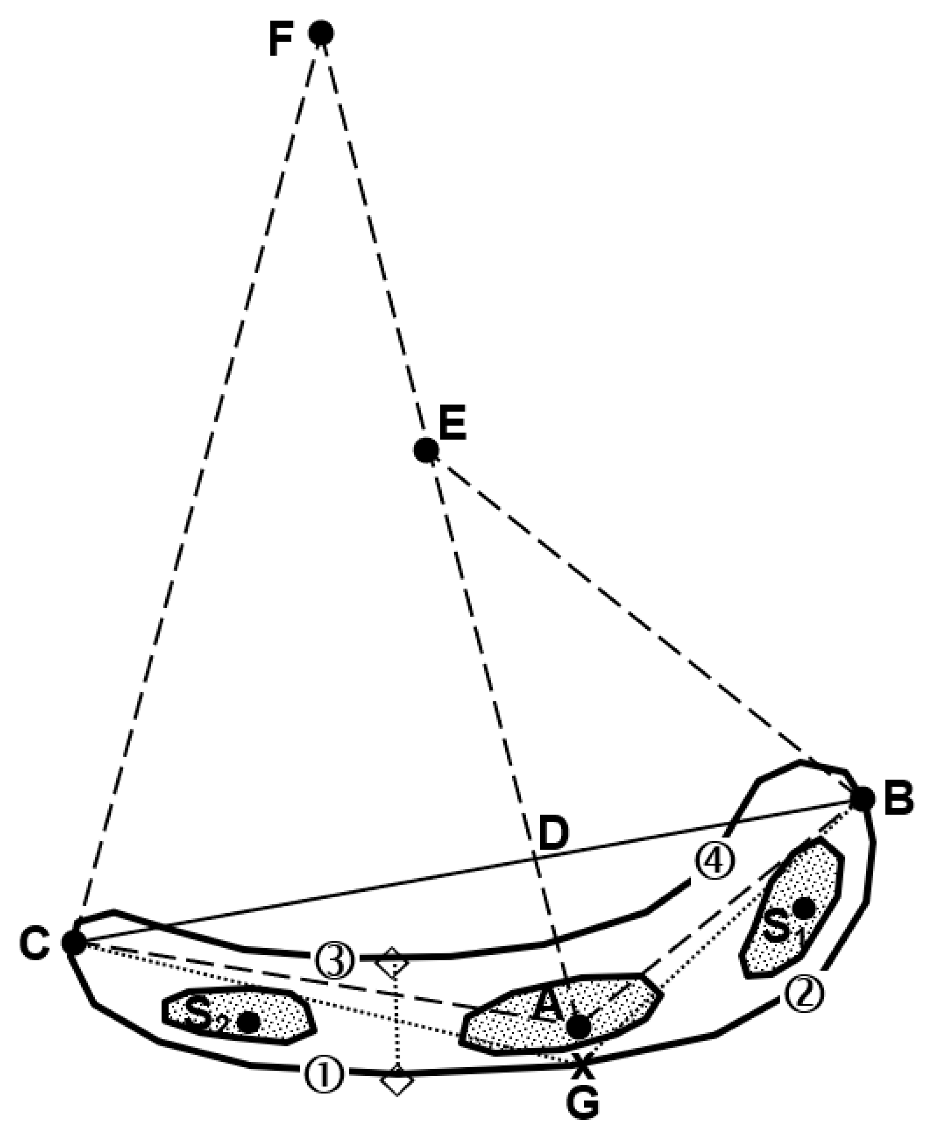
3.2. Attribute Parameters of Rainfall Objects

In the present study, the attribute parameters of rainfall objects considered include the following: (1) total water production; (2) total number of grid points (or area size); (3) average rainfall (among the grid points); (4) maximum rainfall within the object; (5) the location of the maximum rainfall; (6) the rainfall values at five percentiles: 90, 75, 50, 25, 10 (in mm per 3 h); (7) the centroid location of the object, which is the average latitude/longitude of all grid points in the object; (8) the long-axis and short-axis length of the object; (9) the aspect ratio (i.e., the ratio of long axis to short axis) that distinguishes whether the object is quasi-linear or more circular; and (10) the object orientation, i.e., the direction of the long axis on the xy plane (in degrees). This angle is defined to be measured counter-clockwise from the x-axis, so the angle is 0° when the object is aligned along the E–W direction and positive when the object is aligned along the NE–SW direction. The angle can vary between ±90°. A more general treatment of the object orientation may be found in Ritter and Wilson [48]. (11) The curvature of the object: This parameter provides a measure of overall deviation from the straightness of an object, and it is defined as 100 km divided by the radius of curvature of the object (and thus is dimensionless) in this study. This attribute can be used to distinguish whether an object has an arc or bow shape and is useful to characterize the mode of mesoscale convective systems. (12) The object apex location: For an arc-shaped object, it gives the grid-point position of the apex as a reference. As one can see, attributes (1)–(6) describe object size, rainfall amount, and rainfall intensity; attribute (7) gives location; and (8)–(12) characterize the shape and alignment of objects.

Several other attributes are also computed, and some of them are tailored for Taiwan: (13) The number of grid points of the object along the four lateral boundaries of the verification domain, and the numbers of grid points of the object over land and over Taiwan, respectively. For a relatively small verification domain as in the present study, these attributes can indicate whether an object intersects with the domain (and some part of it is outside the domain) or quantify the fraction of objects over land or ocean. (14) The average location of all grid points of the object on the island of Taiwan, which can be used to isolate the objects causing precipitation in different parts of Taiwan in the future; (15) The number of rainfall sub-centers contained in the object; and (16) the ranking of the object among all objects in the same 2D field. The standard used for sorting rainfall objects is total water production, i.e., attribute (1), and this rank will be used to determine the priority or order in the matching procedure to be described in Section 3.3.

While the calculations of many attributes listed above are easy, some of them are not as straight-forward. In Figure 2, a schematic is presented to facilitate the description here. As shown, for the long axis of an object, it is defined in this study as the line between the two farthest points along its boundary (endpoints B and C in Figure 2). The distance and direction obtained by this line (i.e., BC) are the length and orientation of the long axis. To obtain the length of the short axis, a more accurate calculation is done. With the apex identified (marked by an “x”, or point G) as the point on the boundary having the longest total distance to points B and C (i.e., maximum value of BG + CG), the object boundary between B and C can be separated into two segments: those at the front side containing point G, and those at the back side without point G (Figure 2). Then, the two grid points half-way from point G along the front-side segment are identified (marked as ① and ②), and for each grid point between them, the shortest distance to the back-side segment (between ③ and ④) is searched and found. Finally, the short axis is the mean distance of all these lines, one of which is depicted as the dashed line connecting the two diamond symbols in Figure 2. In other words, the length of the short axis is the average distance between two closest points across the long axis direction within a certain range around the apex. For small objects with fewer than 10 grid points along the boundary, the above elaborated method is not necessary, and its short-axis length is simply estimated by dividing the area by the long-axis length.

The curvature is inversely proportional to the radius of curvature of the object. From the definition assumed above, it is seen that the curvature value is less than 1 if the radius of curvature of the object is greater than 100 km, and greater than 1 otherwise. The calculation of the radius of curvature employs a geometric method also illustrated in Figure 2. In the figure, point A has the maximum rainfall value in the object, and line AF intersects line BC (or the long axis) perpendicularly at point D. Then, make line BE normal to line AB from point B (to intersect the extension of AD at point E) and similarly, line CF normal to line AC from point C. Finally, the average length of lines BE and CF is considered the radius of object curvature. In this method, once the three points A, B, and C (thus the lengths of AB, AC, and BC) are known, the position of point D, and thus the lengths of BD and CD, can be obtained through the Pythagorean Theorem on the two right triangles ABD and ACD. Since ∠AEB = ∠ABD and ∠AFC = ∠ACD, the lengths of line BE and CF can be obtained through triangles ABD and ACD using the scalability principle, i.e., BE = AB × BD/AD and CF = AC × CD/AD.

3.3. Matching Procedure for Rainfall Objects

When the rainfall objects are identified in both observations and forecasts, their various attributes can be compared for similarities and differences as part of the verification. To further understand the forecast quality of the model, a matching (or pairing) procedure is used to establish a one-to-one relationship between the observed and forecast objects, i.e., which observed object corresponds to which one in the QPF. In fact, three types of matching are considered in this study, largely based on Davis et al. [19,25]. They are (a) matching between observed and forecast objects at the same time, as the example given above; (b) matching of objects between two successive times in the same dataset (observation or QPF), so as to identify the mesoscale rainfall systems (MRSs) such as the mesoscale convective systems (MCSs) that last through multiple times in each dataset; and (c) matching between observed and forecast MRSs that occur in close proximity in space and time.

For these three types of matching, the procedure is similar (but not without differences), and there are at least two rounds in the process. The first round is to match the candidate pairs of objects (from two different fields) with high certainty using more stringent criteria, and the second round matches the remaining candidate pairs that meet the minimum requirements, i.e., accept the pairs with less certainty but still reasonably similar. To some extent, such a process mimics the behavior of humans. Further details on the matching procedure of each type and their differences are given below.

3.3.1. Matching between Observed and Modeled Objects Occurring at the Same Time

After the objects are identified and their attribute parameters are obtained in both the observed and QPF datasets, the first type of matching to be performed is between the objects in the two datasets occurring at the same time. Similar to Davis et al. [19,25], a series of scores are designed to reflect the similarity between certain attributes of two objects, and the closer the attributes, the higher the score. Then, the total score of two candidate objects under consideration is used to judge whether they can be matched or not (i.e., if they are overall similar enough). The first and the most important parameter considered is the distance between the centroid of two objects (D), and the maximum value allowed (D_max) and the score (S_D) are calculated as

$$D_{max}=\sqrt{A_O}+\sqrt{A_F}$$

(1)

$$S_D=\sqrt{\left(D_{max}-D\right)/D_{max}}·S_{D0}$$

(2)

where A_O is the area of the observed object, A_F is the area of the forecast object, and the square root of each of them represents their characteristic length. When the centroid distance D of two objects under consideration is less than D_max (the maximum distance allowed), the score S_D can be obtained from Equation (2), where S_D0 is the base (maximum) score assigned to this distance parameter (set to four points here). Therefore, the shorter the centroid distance between the two objects, the higher the score. As shown above, D_max is determined by the area size of the two objects, and it is shorter and more difficult to yield a higher score for small objects [19]. If the centroid distance D exceeds D_max or an additional limit of 300 km imposed, the score S_D is zero. In this case, as D is too far for the two objects to be considered eligible for matching as a pair, further calculation of scores for other attributes is not needed and a total score of 0 is assigned.

In Davis et al. [19,25], the centroid distance is the only parameter considered for matching. In this study, however, other parameters are also used to evaluate the overall similarity between two objects. One of them is the orientation of the long axis of the object, and a similar formula is used as

$$S_O=\sqrt{({90}^{°}-|O_O-O_F|)/{90}^{°}}·S_{O0}$$

(3)

where O_O and O_F are the orientation angle of the observed and forecast objects, respectively, their absolute difference is |O_O − O_F|, and S_O0 is the base score for the orientation (and set to one point). Except for centroid distance and orientation, six other attributes (object area, total water production, maximum rainfall, mean rainfall, aspect ratio, and curvature) are also used to constitute the total score, and a common formula in the form below is used:

$$S_A=\sqrt{A_S/A_L}·S_{A0}$$

(4)

where A_S is the smaller value of an attribute parameter between the two objects and A_L is the larger one, while S_A is the score and S_A0 is the base score. The use of squared root in Equations (2)–(4) ensures that relative smaller differences would not affect the score too much. For object area size, S_A0 is set to 2, and it is set to 1 for all five remaining attribute parameters. The total score is simply the sum of all scores from all selected attribute parameters and is thus 12 here, as listed in

Table 2. Summary of object attributes and parameters selected, their base score (points), maximum total score, equation to compute score, and the criteria used in different rounds for the three types of matching: between observed and modeled objects at the same time (Section 3.3.1) between objects in successive times in the same dataset (Section 3.3.2) and between observed and modeled mesoscale rainfall systems (MRSs) (Section 3.3.3). Additional requirements are marked by superscripts, with their meaning given at the bottom.

Type of Matching	Type 1	Type 2		Type 3	Equation
Round in Procedure		Rounds 1/2	Round 3
Attribute/parameter
Centroid distance	4 *	4 *,@	4 *	4 *	(1), (2) or (5) $
Area size	2	2	2	2	(4) or (6) $
Total water production	1	1	1	1	(4) or (6) $
Mean rainfall	1	1		1	(4)
Maximum rainfall	1	1		1	(4)
Aspect ratio	1	1		1	(4)
Long-axis orientation	1	1		1	(3)
Curvature	1	1		1	(4)
Mid-point difference in lifespan				4 #	(7)
Lifetime duration				4	(4)
Maximum total score	12	12	7	20
Criteria for Matching
Round 1	≥9 ^	≥10 ^		≥16 ^
Round 2	≥6	≥7		≥12
Round 3			≥3.5

Meaning of superscripts: *: D ≤ D_max ≤ 300 km; @: object cannot move westward or northward for over 120 km in 3 h; #: ∆T ≤ ∆T_max ≤ 6 h; ^: match must be best-fit for each other; $: Equations (5) and (6) are used only in round 3 of type 2 (between objects and sub-centers at two successive times).

(for type 1).

For the first types of matching, only two rounds are used in the procedure. As described earlier, the first round matches the candidate object pairs with at least 9 points in the total score (out of 12), starting from the highest ranked object (in the two fields involved) and gradually moving down in ranks. For any object, it is matched with the object (from the other field) having the highest total score with one additional requirement: that they must be the mutually best-fit for each other, i.e., there is no better option for either object. After the first round, a second round matches objects with a lower certainty but still quite similar, with at least six points in total score (cf. Table 2), again from the highest to the lowest rank (without the mutual condition). Thus, higher ranked objects always have priority over lower ranked ones in the process, both to be searched for a match and to be considered as a match. Naturally, once two objects are successfully matched, they become ineligible for any possible matching with other objects. In Table 2, a summary for the matching procedure is provided (also for the other two types of matching described later). After two rounds, the matched pairs can be considered “hits” (observed and also predicted objects), and those not matched are either “misses” (objects in observation but not predicted) or “false alarms” (objects in model but not observed).

3.3.2. Matching of Objects between Successive Times in the Same Dataset

The second type of matching, as mentioned, is used to identify rainfall systems through time, so it is done between objects from two successive times in the same dataset (either observation or model). The same formula as Equations (1)–(4) are used for the same set of selected attribute parameters (cf. Table 2, for type 2), except that the subscripts O and F are now replaced by 1 and 2 for the two time frames, which are 3 h apart here. The first two rounds of matching procedure used here are also identical to those described earlier in Section 3.3.1, except for the following differences: First, while an upper limit of 300 km remains for D_max, an object cannot move westward or northward for more than 120 km in 3 h (i.e., 40 km h⁻¹) to be matched (considered the same system). Second, the higher criteria of 10 points and seven points are used in rounds one and two (Table 2), respectively, since now the matched pair is considered the same rainfall system evolving through time, instead of “a similar pair of objects” in two opposing data fields. When an MRS is identified, its lifespan is the number of consecutive time frames that it appears, multiplied by the time interval, so that it must be dividable by 3 h. Then, the mean attributes throughout its lifespan are also computed [25].

In the present case of MRS identification, however, there is a third round that does not affect the matching result but rather provides additional information on the generation of new objects and dissipation of old ones (i.e., on the evolution of MRSs). In this round, using the attribute information on the sub-centers of objects, any unmatched object in the later time is matched with sub-centers in the earlier time to determine whether it splits from an existing object (if paired with a sub-center of that object) or is a newborn object (if not paired). Likewise, unmatched objects in the earlier time are matched with sub-centers in the later time to determine whether they merge into another object (if paired) or simply dissipate in the next time (if not paired). For this purpose, only three attributes are included (centroid distance, area size, and total water production) using the following two equations (with no squared root), as the other attributes (between an object and a sub-center) are not suitable:

$$S_D=\left((D_{max}-D\right)/D_{max})·S_{D0}$$

(5)

$$S_A=\left(A_S/A_L\right)·S_{A0}$$

(6)

With the same base points for consistency (Table 2), the three attributes yield a highest total score of 7, and a score of 3.5 is sufficient for a match. The information from this third round of matching can be useful when the characteristics of MRSs in the observed or modeled fields are analyzed.

3.3.3. Matching between Observed and Modeled Mesoscale Rainfall Systems

After all the MRSs are identified in both the observed and model fields, as described above, they can also be matched to find their correspondence, i.e., whether an observed MRS is predicted by the model, or vice versa. Thus, this third type of matching is performed between observed and forecast MRSs that occur in close proximity in space and time. Here, the same set of attribute parameters as for matching objects are considered, with 12 highest base points (Table 2, for type 3), except that the mean attributes during the lifespan of MRSs are used instead. Two new parameters are introduced. The first is the lifespan duration of the MRS, and equation (4) is used to compute its score, with S_A0 set to four points (Table 2). The other parameter is the (absolute) time difference between the two mid-points in their lifespan (∆T), and the score (S_∆T) is calculated in the same way as Equation (2), such that

$$S_{∆T}=\sqrt{\left(∆T_{max}-∆T\right)/∆T_{max}}·S_{∆T0}$$

(7)

where ∆T_max is the maximum time difference allowed between the two lifespan mid-points and it is set to 6 h, beyond which a successfully pairing cannot occur (as in the case of D > 300 km). The base score (S_∆T0) is also four points, such that the highest total points are 20 (see Table 2).

For the pairing of MRSs, a similar matching procedure with two rounds are also used. As before, the priority of MRSs in each round depends on their ranking, which is now based on the total water production during their lifetime. As the MRSs may overlap in time, which runs continuously, data of all MRSs during the entire data period (1.5 months in this case) in both datasets are entered simultaneously for matching, but only those potential pairs with D ≤ D_max ≤ 300 km and ∆T ≤ ∆T_max ≤ 6 h are eligible. In the first round, the matching criterion is 16 points and the requirement of mutual best-fit is also imposed. In the second round, the criterion is lowered to 12 points (Table 2).

4. Assessment of the Developed Verification Method

In this section, the applicability of the developed object-based verification method is assessed. The SoWMEX field phase in May–June 2008 (47 days), when extensive Mei-yu rainfall occurred in and near Taiwan, is chosen as the target period in association with the forecasts provided by the CReSS model. The overall distribution of the key attributes of both observed and forecast objects are compared for both cases before and after matching. The comparisons between the climatology of observed rainfall features and that of the features produced by the model can be extremely informative. Biases inherent in the distributions of object characteristics can reveal systematic errors in certain aspects and can be helpful to improve weather and climate models.

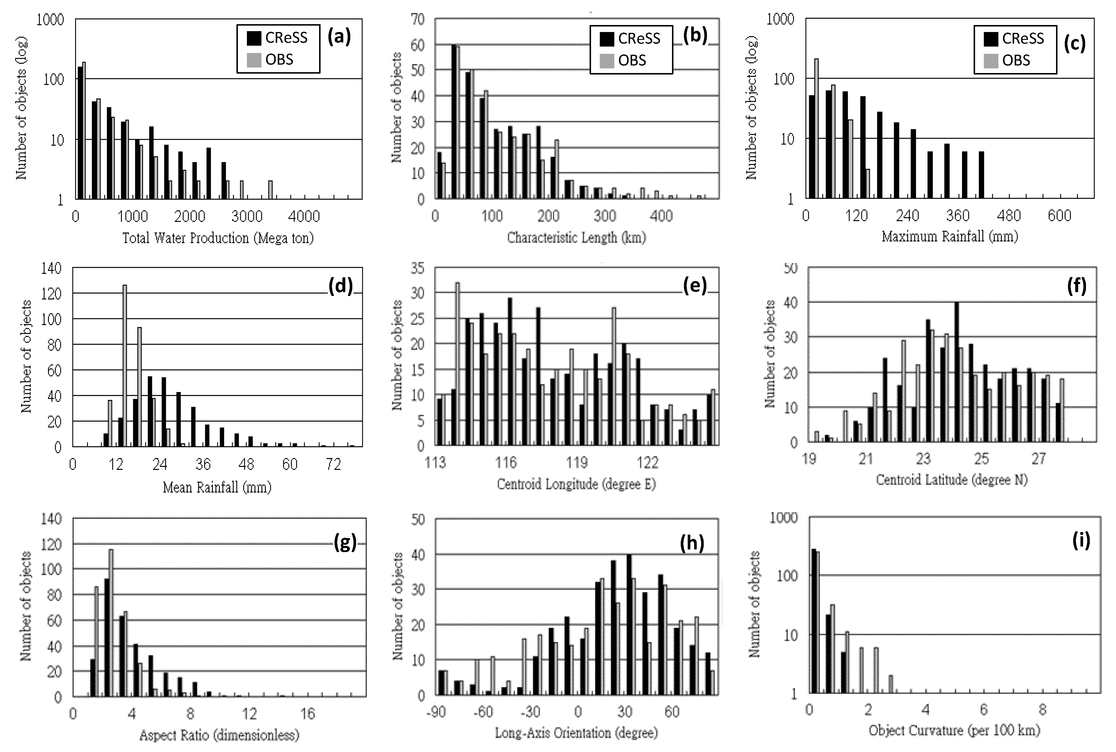
4.1. Evaluation on Object Properties without Matching

During the 47-day data period, the twice daily CReSS QPFs (initialized at 00:00 and 12:00 UTC), every 3 h over the range of 0–48 h, produced a total of 8642 objects (5.75 objects per 2D rainfall field). The number of objects in observation is 6081 (4.04 objects per field) during the corresponding time periods, which is four times the length in reality (since the model generates 96 h of output data per day). In this Section, the statistical distributions of the number of observed and forecast objects stratified based on the values of relevant attributes, such as those linked to object size, rainfall intensity, location, shape, and orientation, before matching are presented in Figure 3 using histograms. The average value and standard deviation (SD) of these attributes are given in

Table 3. Mean value and standard deviation (SD) of major attributes of the rainfall objects (at 3-h intervals) in observation and CReSS forecasts (initialized twice daily at 00:00 and 12:00 UTC, each for 48 h). The observed number of objects, at 6081, is for the same time periods as all the forecasts.

Parameter	Observation		CReSS
	Mean	SD	Mean	SD
Total number of objects	6081		8642
Total water production (106 ton)	157.2	383.7	174.5	380.5
Area size (km2)	7494	13,041.1	5875.5	11,708.2
Mean rainfall (mm)	3.9	2.6	23.8	9
Maximum rainfall (mm)	29	21.3	84.1	75.6
90-percentile of rainfall (mm)	4.6	2.7	49.6	29.9
75-percentile of rainfall (mm)	4.2	2.7	32.4	14.2
50-percentile of rainfall (mm)	3.6	2.4	18.7	4.6
25-percentile of rainfall (mm)	2.3	2.2	11.6	3.2
10-percentile of rainfall (mm)	2	3	8.1	4
Centroid longitude (° E)	118.24	3.45	118.37	2.95
Centroid latitude (° N)	23.94	2.33	24.68	1.94
Long-axis orientation (°)	13.6	49.2	17.3	42.9
Long-axis length (km)	118.1	133.3	114.8	128.4
Short-axis length (km)	44.1	38.2	34.4	29.6
Aspect ratio	2.5	1.1	3	1.71
Curvature (10−2)	0.93	1.87	0.6	1.43
Number of sub-centers	0.24	0.65	0.81	1.16

.

All histograms of the distributions of attributes linked to object size and rainfall intensity, such as total water production, characteristic length (squared root of area size), and peak rainfall, show a pattern perhaps similar to a χ distribution, with a single peak (the most number of objects) at a fairly small value than decreased number of objects toward higher values (Figure 3a–c, and also for the observed objects in Figure 3d). While CReSS produces roughly 40% more objects, the distribution of the characteristic length is very similar to that in observation, both with a peak at 20–40 km and very few objects reaching 300 km in length (Figure 3b). In terms of total water output, however, CReSS have more objects in the middle of the spectrum (about 1500–3000 megatons) than observation, and the opposite is true at the higher range above 3000 megatons (even though the number of objects become very low there). In Figure 3c, the CReSS model produces a much greater number of objects with maximum rainfall over 200 mm per 3 h (and even up to 600 mm), but none of the observed objects can reach a peak rainfall of 200 mm. While it explains the higher water outputs in CReSS in Figure 3a (over the middle range), this significant difference in fact may be largely due to the higher resolution of CReSS compared to the coarser TRMM data that constitute the majority of rainfall observations in the verification domain. Even over Taiwan, the Cressman objective analysis used is an interpolation scheme, which tends to smooth out the peak value observed at stations. Thus, in the histogram of mean rainfall (Figure 3d), the objects in CReSS peak at 20–24 mm per 3 h (and it can reach about 50 mm, also per 3 h), significantly higher than the observation. In Table 3, the CReSS is also seen to produce stronger rainfall, but its objects have a smaller average size compared to observation, whose objects tend to be bigger in size but often contain many grid points with weak rainfall. Thus, this apparent over-forecast by CReSS in rainfall intensity deserves to be explored further also using other verification methods. The results obtained with this further investigation are reported in Part I [24] and Part III [49].

For object centroid locations, the distribution of observed object numbers with respect to centroid longitude show a double-peak structure, with one peak near 115° E and the other around 121° E (Figure 3e). The pattern produced by CReSS also has two peaks, but the one to the west is near 117° E instead, with an excessive number of objects over the range of about 115.5–119.5° E compared to observation. The distributions of the observed and modeled centroid latitude perhaps agree somewhat better, both with (roughly) a single peak around 24° N, but again the CReSS model produces more objects than observed at 24°–27° N (Figure 3f). This region of excessive number of objects in CReSS is the hilly region in southeastern China (cf. Figure 1e), so the terrain there may arguably have some influence. The frequency peak in the object number to the east near 24° N, 121° E is directly over Taiwan, whose steep terrain would most likely exert even a stronger impact to rainfall, as shown by many previous studies [23,32,40,50].

Figure 3g–i illustrates the distributions of object numbers in relation to three shape-related attributes, including aspect ratio, orientation of long axis, and curvature. In the histogram for aspect ratio, the distributions of both observed and modeled objects show a decreasing pattern with increasing value since about 2, but CReSS has too many objects with a higher aspect ratio beyond about 5 (and up to about 15, Figure 3g). Thus, there is a tendency in CReSS to produce too many elongated objects, while the observed objects tend to be more rounded in their shape, in agreement with Table 3. For long-axis orientation (Figure 3h), both the observation and CReSS show a higher frequency of objects in the positive side (NE–SW aligned) than negative side (NW–SE aligned) and thus are in general agreement in the overall pattern. However, CReSS predicts many more objects in the range of 10–70° than those observed (even though the mean and SD values are quite similar in Table 3). As Figure 3e,f indicate that most of these excessive objects are in southeastern China, so it is not surprising that they are mostly aligned in a NE–SW direction and roughly parallel to the hilly terrain there. On the other hand, both distributions are highly similar and in close agreement on the negative side. Finally, for the distributions of object curvature, the observed and modeled patterns are similar, with the highest peak at low curvature value (nearly straight) and fewer objects toward higher values (more curved, Figure 3i). Nevertheless, while the majority of objects have a curvature values confined within 10 × 10⁻² (i.e., with a radius of curvature at least 10 km), there are a few observed objects that have a curvature value up to 15–22.5 × 10⁻² (i.e., with a radius less than 7.5 km), which the model forecasts do not have. In Table 3, the objects in the observation also exhibit a higher mean value in their curvature. Apart from this difference, the two distributions in Figure 3i are highly similar. In Table 3, the mean and SD values of the number of sub-centers are also given, and the model (0.81 per object) has about three times as many sub-centers as in the observation, and this is consistent with the more intense and concentrated rainfall provided by CReSS, as discussed earlier.

Overall, the distributions of objects produced by CReSS, in terms of their shape and orientation, agree well with the observation. However, the modeled objects, although not larger in size, tend to be significantly stronger in rainfall (especially in maximum rainfall), leading to higher total water output (Figure 3 and Table 3) due to its high resolution as compared to the TRMM rainfall data. While the CReSS model produces about 2500 more objects than observation, most of them seem to be located near the southeastern coast of China (Figure 3e,f), most likely influenced by the topography in that area.

4.2. Evaluation on the Properties of Matched Object Pairs

When the 12–36-h QPFs from CReSS are extracted, the daily forecasts initialized at 00:00 UTC form a continuous data stream, from 12:00 UTC 15 May to 12:00 UTC 30 June. The modeled rainfall objects in 3-h fields (1834 of them) thus can be matched with the observed objects (1132) over the same period, using the first type of matching procedure (Section 3.3.1, Table 2). Likewise, the model objects produced by 1200-UTC runs (1613 of them) are matched with the observed ones (1141) for the time period shifted by 12 h (i.e., 00:00 UTC 16 May to 00:00 UTC 1 July). Each data period lasts 46 days, and a total of 309 and 295 objects for 00:00- and 12:00-UTC CReSS model runs, respectively, are successfully matched with the observed objects. The histograms of major attributes for these matched object pairs are presented and discussed below.

The attributes selected here are the same as those included in Figure 3, and the histograms for the 00:00-UTC runs are shown in Figure 4 and their mean values are summarized in

Table 4. Mean value of major attributes of the matched rainfall object pairs (at 3-h intervals) in observation and CReSS forecasts at the range of 12–36 h, initialized daily at 00:00 or 1200 UTC. The data length is the same for both dataset (46 days).

Initial Time	0000 UTC		1200 UTC
Parameter	Observation	CReSS	Observation	CReSS
Total number of matched objects	309	309	295	295
Total water production (106 ton)	411.3	531.6	412.9	475.8
Area size (km2)	21,573.2	16,873.6	22,033.3	15,255.2
Mean rainfall (mm)	16.3	27.8	16.2	28.1
Maximum rainfall (mm)	37.8	131.2	36.9	130.7
90-percentile of rainfall (mm)	24	60.1	23.9	61.2
75-percentile of rainfall (mm)	19.5	36.9	19.4	37.3
50-percentile of rainfall (mm)	15.2	20.2	15.1	20.2
25-percentile of rainfall (mm)	12.2	11.9	12.2	11.9
10-percentile of rainfall (mm)	10.5	8	10.4	8.1
Centroid longitude (° E)	117.94	118.11	117.64	117.77
Centroid latitude (° N)	24.18	24.36	24.35	24.53
Long-axis orientation (°)	16.5	25	14.9	23.5
Long-axis length (km)	216.7	250.5	223.4	214.7
Short-axis length (km)	73.1	61	72.4	58.9
Aspect ratio	2.8	4.1	2.9	3.7
Curvature (10−2)	0.38	0.25	0.37	0.2
Number of sub-centers	0.58	1.73	0.57	1.49

. For attributes linked to object size (total water production and characteristics length), the CReSS model performs well (Figure 4a,b), as the differences between distributions in model and observation are small (as compared to the differences before matching in Figure 3) with the same number of objects (309). Nonetheless, CReSS still tends to produce more objects above 1000 megatons (Figure 4a) and exhibits a slightly higher mean water output than observed, but the averaged size remains slightly smaller (Table 4). For a higher water yield to occur in CReSS for paired objects, the model’s distributions for both maximum and mean rainfall must shift toward the heavy side compared to the observation in their histogram (Figure 4c,d) as expected and in agreement with the information given in Table 4 (including the rainfall values at various percentiles). Of course, this tendency for CReSS to produce rainfall objects with higher peak and mean rainfall values is also evident above in Figure 3, as already pointed out. However, the distinct differences between model and observation are reduced after matching, especially in mean rainfall (Figure 4d) as the observed objects now have higher mean rainfall values that peak at 12–16 mm (also cf. Table 4 and Figure 3d). Thus, the objects with more intense rainfall in the observation have a higher chance to be matched with an object in CReSS, as intended.

The histograms of the centroid longitude and latitude (Figure 4e,f) of matched objects reveal similar patterns in CReSS and observation as expected, since the centroid distance is the most important parameter considered and poses a stringent criterion in type-1 matching, especially for smaller objects. Compared to the distribution before matching (cf. Figure 3e,f), it is seen that most of the excessive objects with a centroid latitude/longitude within 24–27° N, 116–119.5° E in CReSS are not successfully matched (Figure 4e,f), a reasonable result because relatively few objects are located there (near the southeastern coast of China) in the observation.

For the three attributes related to shape and orientation, the distributions are in reasonable agreement between model and observation even before matching (cf. Figure 3g–i), as mentioned. After matching, the agreements in their patterns in aspect ratio and orientation further improve (Figure 4g,h), as one might expect. The matched objects in CReSS, however, still tend to exhibit slightly higher aspect ratios than in observation, but now only objects with an aspect ratio between 1 and 12 can be matched (Figure 4g). The patterns in orientation also show better agreement, with significantly more objects with a positive angle of alignment than those with a negative angle, without the excessive objects over southeastern China (Figure 4h). For curvature (Figure 4i), the matched objects exclusively have values less than 3 × 10⁻² (with a curvature radius longer than 33 km). Hence, the highly curved objects (which must be very small) cannot be matched, while the curvature of observed objects still tend to be slightly higher. The above distributions in shape-related attributes are also in agreement with Table 4.

For comparison, the histograms for the same nine attributes of the 295 paired objects between the observation and model 12–36-h QPFS initialized once per day at 1200 UTC are presented in Figure 5, and their mean values are given also in Table 4 (two columns to the right). Although a different set of model forecast data (12:00-UTC runs) are used, all the distributions remain highly similar to those in Figure 4 and Table 4 from 00:00-UTC runs, since the data period used is only shifted by 12 h.

4.3. Evaluation on the Properties of MRSs in the Observation and Model Forecasts

In this section, the properties and characteristics of MRSs that last for at least 3 h, as identified by the second type of matching (Section 3.3.2, Table 2), in both the observation and QPFs (at the range of 12–36 h), are compared. In the 46-day time series of rainfall objects (at 3-h intervals), there are 607 and 868 MRSs (from 1132 and 1834 rainfall objects) in the observation and 00:00-UTC forecasts, and 631 and 756 MRSs (from 1141 and 1613 objects) in the observation and 12:00-UTC runs, respectively. At the same order, the average lifespans (i.e., durations) of MRSs are 5.58, 6.33, 5.43, and 6.39 h, respectively. The greater numbers of MRSs here than the matched pairs in Table 4 (by at least two folds) suggest that the success rate for matching in type 2 is higher than that in type 1, despite more stringent criteria (cf. Table 2). Following Davis et al. [25], the mean values of attributes during the lifetime of MRSs are shown in the histograms as well as in

Table 5. Mean value of major attributes of MRSs (from data at 3-h intervals) in observation and CReSS forecasts at the range of 12–36 h, initialized daily at 00:00 or 12:00 UTC. For each MRS, the attributes are averaged during its lifetime.

Initial Time	0000 UTC		1200 UTC
Parameter	Observation	CReSS	Observation	CReSS
Total number of MRSs	607	868	631	756
Total water production (106 ton)	103.3	115.5	102.9	99.1
Area size (km2)	6008.5	4046.8	5894.6	3470.6
Mean rainfall (mm)	13.9	21.9	13.9	21.6
Maximum rainfall (mm)	25.2	69.1	25.5	65
90-percentile of rainfall (mm)	19	43.5	19.2	42.5
75-percentile of rainfall (mm)	16.2	29.3	16.3	29.1
50-percentile of rainfall (mm)	13.3	17.9	13.4	17.9
25-percentile of rainfall (mm)	11.4	11.8	11.4	11.9
10-percentile of rainfall (mm)	10.2	8.7	10.1	8.8
Centroid longitude (° E)	118.19	118.42	118.16	118.41
Centroid latitude (° N)	24.06	24.6	24.12	24.64
Long-axis orientation (°)	12.7	17.8	13.4	18.3
Long-axis length (km)	94.5	92.5	93.5	82.8
Short-axis length (km)	36.3	28.2	35.5	26.8
Aspect ratio	2.4	2.9	2.4	2.8
Curvature (10−2)	1.14	0.77	1.15	0.9
Number of sub-centers	0.16	0.6	0.16	0.52

below.

Between the 00:00-UTC forecasts and the observation, the distributions of the numbers of MRSs in the histograms for most of the attributes (Figure 6) are quite similar to those for paired objects in Figure 4, with generally good agreement between the observation and model forecasts, if one neglects the difference in MRS/object numbers. This is perhaps not surprising, since the procedures used for type-1 and type-2 matching are essentially the same, except for the difference in criteria and one additional requirement (Table 2). For example, the mean and maximum rainfall in CReSS MRSs remain higher than in those observed (Figure 6c,d). However, as also reflected by the patterns in characteristic length, the mean area size of MRSs (Table 5) is significantly reduced and even become smaller than the value before any matching (cf. Table 3). This finding indicates that some of the smaller objects (likely rather slow in movement) can be matched in successive times, or perhaps at early or late stage of MRSs. The histogram for the long-axis length is also plotted (Figure 6e) and suggests good agreement between the observation and model prediction, as for the curvature (Figure 6h). Since the MRSs in the model and observation are identified independently here, the histograms for aspect ratio and long-axis orientation again exhibit the same characteristics as in Figure 3g,h, such as the tendency to produce MRSs with a higher aspect ratio (Figure 6f) or an excessive number of MRSs with a NE–SW orientation (Figure 6g). These features are also expected and quite reasonable. Using the MRSs in CReSS (12–36-h) QPFs initialized at 1200 UTC only, the set of histograms exhibit distributions very similar to those in Figure 6, and thus they are not shown here. The mean values are, however, given in Table 5 for comparison. All these values are very close to those from 00:00-UTC runs.

5. Discussion and Conclusions

In this study, an object-oriented verification method is developed for Taiwan, as a complement to existing conventional methods. The developed method is preliminarily applied for QPF verification during the Mei-yu season. This study describes in detail the methodology adopted to (i) identify rainfall objects, (ii) compute their attributes, and (iii) match objects at close proximity with similar properties. Object matching includes comparison between observed and modeled objects at the same time (type 1), between objects at successive times (i.e., to identify MRSs) in the same dataset (either observation or forecast, type 2), and between observed and modeled MRSs (type 3). By merging the rain-gauge data in Taiwan with the TRMM data, a gridded rainfall dataset is created for the field phase of SoWMEX in May-June 2008. This dataset is used to evaluate the twice-daily QPFs at 3-h intervals within a range of 48 h provided by the CReSS model. Rainfall objects in both datasets are identified and matched, and the characteristics in their attributes are compared and discussed both before and after matching.

After convolution (or smoothing), masking by a selected rainfall threshold (10 mm per 3 h), and filtering, rainfall objects in each 2D field (at 3-h intervals) are identified (Section 3.1) and their attributes computed, including total water production, area size, peak rainfall amount and location, areal-mean rainfall, rainfall at selected (90, 75, 50, 25, and 10) percentiles, centroid location, length and orientation of long axis, length of short axis, aspect ratio, curvature, apex location, number of sub-centers (i.e., local rainfall maxima), and several other parameters designed to fit the conditions in Taiwan (Section 3.2). The objects from the same 2D field are also ranked on the basis of total water production, used to determine their priority in the matching procedures. That is, higher-ranked and larger objects have priority over lower-ranked and smaller objects. After the identification of all objects in the data period, the observed and forecast objects at the same time can be matched (type 1, Section 3.3.1), and the successful pairs are considered “hits” by the model. Likewise, objects from the same data source (observation or forecast) can be matched through time to identify MRSs (Section 3.3.2) that last for at least one time level (3 h). The mean attributes of these MRSs are also obtained, and they can be matched between observations and QPFs to identify those systems that appear in close proximity in space and time (Section 3.3.3). The matching processes themselves are based on a score approach, and in principle, candidate object pairs with a shorter distance between their centroids and overall more similar in their attributes can register a higher score, which allows them to be matched once the specified criterion is met (Table 2).

As a preliminary application, the newly-developed object-oriented method is used to evaluate CReSS QPFs during the SoWMEX period (47 days, from 15 May to 30 June) in Section 4.1, and histograms are used to compare the distributions of rainfall objects stratified by attribute values between the observation and forecasts (6081 objects and 8642 objects, respectively). Before matching, in histograms linked to water output, maximum rainfall, object size, characteristic and long-axis length, and aspect ratio, the pattern typically shows a peak in object frequency at a fairly low value and then decreased frequencies toward higher values. The observed and model distributions exhibit reasonable agreement for many attributes, especially those related to object shape, but the CReSS objects tend to have more intense rainfall than the observation, while the latter has a higher percentage of bigger objects with weaker rainfall (Figure 3 and Table 3). The patterns for object centroid location in both the observation and QPFs show relatively high frequencies over and near Taiwan, reflecting the influence of the steep topography. Moreover, they also reveal that the majority of the excessive objects in CReSS (by roughly 2500 in number) are located over the hilly regions in southeastern China and aligned roughly parallel to the local terrain. For long-axis orientation, the CReSS also captures the observed characteristics, that there are more objects aligned in the NE–SW direction and fewer ones aligned in the NW–SE direction (Figure 3). Some of the above results, while revealed using rainfall objects, are in general consistent with the subjective evaluation reported in Part I [24].

The tendency in CReSS to produce smaller but more intense rainfall is presumably linked to its considerably higher resolution, as compared to the coarser TRMM data that constitute the majority of rainfall observations in the verification domain (cf. Figure 1). However, the single domain with a limited size of CReSS means that its results are also sensitive to the IC/BCs from the NCEP GFS, as demonstrated in some previous studies, e.g., Hsiao et al. [51]. Therefore, while the difference in data resolution between model and observation is clearly important, how may the model QPFs change using a different source for IC/BCs [51], or in response to a different grid size, such as Wang et al. [52], or other physical options (e.g., for the PBL parameterization) can also play some role and remain to be explored.

Using the 12–36-h QPFs, the objects from the 3-h fields in the forecasts (at either 00:00 or 12:00 UTC) are matched with those in the observation occurring at the same time (type 1), and the characteristics of these matched pairs are also examined (Section 4.2). Out from a total of 1132 (observed) objects and 1834 (CReSS) objects for the 46-day data period of the 00:00-UTC runs, and 1141 (observed) objects and 1613 (CReSS) objects for the 12:00-UTC runs, 309 pairs and 295 pairs are successfully matched (i.e., identified as “hits” of rainfall objects by the model). As the pairing requires close proximity in distance (relative to their size) and overall similarities between the objects, the distribution patterns between observed and modeled objects in the histograms become better agreed and improved (especially in centroid location), as expected (Figure 4 and Figure 5 and Table 4). The larger objects with higher total water production and heavier rainfall are more easily matched since they have higher priority in the matching process. In addition, they also tend to exhibit smaller curvature values.

Finally, objects in successive times (3 h apart) are matched to identify the MRSs (type 2) through time in both datasets in the observation and model QPFs. A total of 607 MRSs and 868 (631 and 756) MRSs are obtained in the observation and model fields for the 46-day time series corresponding to 00:00-UTC (12:00-UTC) runs, respectively (Section 4.3). The more abundant MRSs in their total number (607–868) compared to the pairs obtained by type-1 matching (309 and 295) indicate that the matching between two adjacent times is easier despite more stringent criteria. Consistent with this, the distributions of average attribute parameters through the lifetime of MRSs, while also showing good agreement between observed and modeled systems (Figure 6), reveal that the size on average is in fact reduced (Table 5), as the matching becomes easier. These smaller MRSs may be stationary or slow-moving, and the size of many MRSs may also be quite small at an early or late stage. Since the MRSs are identified separately in the time series from the observation and QPFs, some of the differences before matching also appear in the histograms of MRSs (such as an excessive number of MRSs over southeastern China). Overall, the current study demonstrates the usefulness of the developed object-based verification method, in providing more detailed information on various aspects regarding the performance in the QPFs from a high-resolution model.

It should be noted that while the method is described in detail, the object-oriented assessment presented in this study represents only preliminary results. The potential for many further applications using such an object-oriented verification method is high. For instance, in Part III [49] of this paper series, the performance of three mesoscale models (including CReSS) are inter-compared. The method can be applied to other rainfall regimes such as typhoon rainfall or afternoon convection. For Mei-yu QPFs like in the present study, there are many places in the method that can be adjusted or amended to improve its usability and suitability in the context of its application. These include the rainfall threshold used for masking (10 mm per 3 h), the maximum limit of centroid distance allowed (300 km), the criteria used for matching, which attributes/parameters to be included as part of the score for matching, and how the scores may be calculated, etc. As it is not possible for a single standard to fit all situations, it is natural for some of the details to be adjusted to better fit the application at hand. As the technique matures, such methods have the potential to provide diagnostic information to forecasters and model users and developers, and also help to meet the decision-making needs for a wide variety of users.

References

1. Fritsch, J.M.; Hauze, R.A., Jr.; Adler, R.; Bluestein, H. Quantitative precipitation forecasting: Report of the Eighth Prospectus Development Team, U.S. Weather Research Program. Bull. Am. Meteorol. Soc. 1998, 79, 285–299. [Google Scholar] [CrossRef]
2. Golding, B.W. Quantitative precipitation forecasting in the UK. J. Hydrol. 2000, 239, 286–305. [Google Scholar] [CrossRef]
3. Schaefer, J.T. The critical success index as an indicator of warning skill. Weather Forecast 1990, 5, 570–575. [Google Scholar] [CrossRef] [Green Version]
4. Doswell, C.A.; Davies-Jones, R.; Keller, D.K. On summary measures of skills in rare event forecasting based on contingency tables. Weather Forecast 1990, 5, 576–585. [Google Scholar] [CrossRef] [Green Version]
5. Mesinger, F.; Black, T.L. On the impact on forecast accuracy of the step-mountain (eta) vs. sigma coordinate. Meteorol. Atmos. Phys. 1992, 50, 47–60. [Google Scholar] [CrossRef]
6. Wilks, D.S. Statistical Methods in the Atmospheric Sciences; Academic Press: Cambridge, MA, USA, 1995; p. 704. [Google Scholar]
7. Chien, F.C.; Kuo, Y.H.; Yang, M.J. Precipitation forecast of MM5 in the Taiwan area during the 1998 Mei-yu season. Weather Forecast 2002, 17, 739–754. [Google Scholar] [CrossRef]
8. Chien, F.C.; Jou, B.J.D. MM5 ensemble mean precipitation forecast in the Taiwan area for three early summer convective (Mei-Yu) seasons. Weather Forecast 2004, 19, 735–750. [Google Scholar] [CrossRef]
9. Murphy, A.H. Forecast verification: Its complexity and dimensionality. Mon. Weather Rev. 1991, 119, 1590–1601. [Google Scholar] [CrossRef]
10. Olson, D.A.; Junker, N.W.; Korty, B. Evaluation of 33 years of quantitative precipitation forecasting at the NMC. Weather Forecast 1995, 10, 498–511. [Google Scholar] [CrossRef] [Green Version]
11. Chen, G.T.J. On the forecast skill of heavy rainfall in Taiwan. Atmos. Sci. 1991, 19, 188. [Google Scholar]
12. Hong, J.S. Evaluation of the high-resolution model forecasts over the Taiwan area during GIMEX. Weather Forecast 2003, 18, 836–846. [Google Scholar] [CrossRef]
13. Chien, F.C.; Liu, Y.C.; Jou, B.J.D. MM5 ensemble mean forecasts in the Taiwan area for the 2003 Mei-Yu season. Weather Forecast 2006, 21, 1006–1023. [Google Scholar] [CrossRef] [Green Version]
14. Brooks, H.E.; Doswell, C.A., III. A comparison of measures-oriented and distributions-oriented approaches to forecast verification. Weather Forecast 1996, 11, 288–303. [Google Scholar] [CrossRef]
15. Ebert, E.E.; McBride, J.L. Verification of precipitation in weather systems: Determination of systematic errors. J. Hydrol. 2000, 239, 179–202. [Google Scholar] [CrossRef]
16. Roberts, N.M.; Lean, H.W. Scale-selective verification of rainfall accumulations from high-resolution forecasts of convective events. Mon. Weather Rev. 2008, 136, 78–97. [Google Scholar] [CrossRef]
17. Mass, C.F.; Ovens, D.; Westrick, K.; Colle, B.A. Does increasing horizontal resolution produce more skillful forecasts? Bull. Am. Meteorol. Soc. 2002, 83, 407–430. [Google Scholar] [CrossRef]
18. Brown, B.G.; Bullock, R.; Davis, C.; Manning, K.; Morss, R.; Mueller, C. An object-based diagnostic approach for QPF and convective forecast verification. In Proceedings of the Workshop on Making Verification More Meaningful, Boulder, CO, USA, 30 July–1 August 2002. [Google Scholar]
19. Davis, C.; Brown, B.; Bullock, R. Object-based verification of precipitation forecasts. Part I: Methodology and application to mesoscale rain areas. Mon. Weather Rev. 2006, 134, 1772–1784. [Google Scholar] [CrossRef] [Green Version]
20. Ebert, E.E. Verifying satellite precipitation estimates for weather and hydrological applications. In Proceedings of the 1st International Precipitation Working Group (IPWG) Workshop, Madrid, Spain, 23–27 September 2002. [Google Scholar]
21. Kain, J.S.; Baldwin, M.E.; Janish, P.R.; Weiss, S.J.; Kay, M.P.; Carbin, G.W. Subjective verification of numerical models as a component of a broader interaction between research and operations. Weather Forecast 2003, 18, 847–860. [Google Scholar] [CrossRef] [Green Version]
22. Knievel, J.C.; Ahijevych, D.A.; Manning, K.W. Using temporal modes of rainfall to evaluate the performance of a numerical weather prediction model. Mon. Weather Rev. 2004, 132, 2995–3009. [Google Scholar] [CrossRef] [Green Version]
23. Wang, C.C.; Chien, F.C.; Paul, S.; Lee, D.I.; Chuang, P.Y. An evaluation of WRF rainfall forecasts in Taiwan during three Mei-yu seasons of 2008–2010. Weather Forecast 2017, 32, 1329–1351. [Google Scholar] [CrossRef]
24. Paul, S.; Wang, C.C.; Tseng, L.S.; Lee, D.I. Evaluation of rainfall forecasts by three mesoscale models during the Mei-yu season of 2008 in Taiwan. Part I: Subjective comparison. Asia Pac. J. Atmos. Sci. under review.
25. Davis, C.; Brown, B.; Rullock, R. Object-based verification of precipitation forecasts. Part II: Application to convective rain systems. Mon. Weather Rev. 2006, 134, 1785–1795. [Google Scholar] [CrossRef] [Green Version]
26. Ebert, E.E. Fuzzy verification in high resolution gridded forecasts: A review and proposed framework. Meteorol. Appl. 2008, 15, 51–64. [Google Scholar] [CrossRef]
27. Gilleland, E.; Lindström, J.; Lindgren, F. Analyzing the image warp forecast verification method on precipitation fields from the ICP. Weather Forecast 2010, 25, 1249–1262. [Google Scholar] [CrossRef]
28. Wang, C.C. On the calculation and correction of equitable threat score for model quantitative precipitation forecasts for small verification areas: The example of Taiwan. Weather Forecast 2014, 29, 788–798. [Google Scholar] [CrossRef]
29. Cortesi, N.; Gonzalez-Hidalgo, J.C.; Trigo, R.M.; Ramos, A.M. Weather types and spatial variability of precipitation in the Iberian Peninsula. Int. J. Clim. 2014, 34, 2661–2677. [Google Scholar] [CrossRef]
30. Foufoula-Georgiou, E.; Vuruputur, V. Patterns and organization in precipitation. In Spatial Patterns in Catchment Hydrology-Observations and Modelling; Grayson, R., Blöschl, G., Eds.; Cambridge University Press: Cambridge, UK, 2001; pp. 82–104. [Google Scholar]
31. Jolliffe, I.T.; Stephenson, D.B. Forecast. Verification: A Practitioner’s Guide in Atmospheric Science; Wiley and Sons: Hoboken, NJ, USA, 2003; p. 240. [Google Scholar]
32. Wang, C.C. The more rain, the better the model performs—The dependency of quantitative precipitation forecast skill on rainfall amount for typhoons in Taiwan. Mon. Weather Rev. 2015, 143, 1732–1748. [Google Scholar] [CrossRef]
33. Shapiro, M.A.; Thorpe, A.J. The observing system research and predictability experiment (THORpex). In Proceedings of the International Conference on Mesoscale Convective Systems and Heavy Rainfall/Snowfall in East Asia, Tokyo, Japan, 29–31 October 2002; pp. 1–12. [Google Scholar]
34. Fritsch, M.J.; Carbone, R.E. Improving quantitative precipitation forecasts in the warm season: A USWRP research and development strategy. Bull. Am. Meteorol. Soc. 2004, 85, 955–965. [Google Scholar] [CrossRef] [Green Version]
35. Ebert, E.E.; Gallus, W.A., Jr. Toward better understanding of the Contiguous Rain Area (CRA) method for spatial forecast verification. Weather Forecast 2009, 24, 1401–1415. [Google Scholar] [CrossRef] [Green Version]
36. Bytheway, J.L.; Kummerow, C.D. Toward an object-based assessment of high-resolution forecasts of long-lived convective precipitation in the central U.S. JAMES 2015, 7, 1248–1264. [Google Scholar] [CrossRef]
37. Giannakaki, P.; Martius, O. An object-based forecast verification tool for synoptic-scale Rossby waveguides. Weather Forecast 2016, 31, 937–946. [Google Scholar] [CrossRef] [Green Version]
38. Jou, B.J.D.; Lee, W.C.; Johnson, R.H. An overview of SoWMEX/TiMREX. In The Global Monsoon System: Research and Forecasts, 2nd ed.; Chang, C.-P., Ed.; World Scientific: Singapore, 2011; pp. 303–318. [Google Scholar] [CrossRef] [Green Version]
39. Hsu, J. ARMTS up and running in Taiwan. Väisälä News 1998, 146, 24–26. [Google Scholar]
40. Chen, T.C.; Yen, M.C.; Hsieh, J.C.; Arritt, R.W. Diurnal and seasonal variations of the rainfall measured by the Automatic Rainfall and Meteorological Telemetry System in Taiwan. Bull. Am. Meteorol. Soc. 1999, 80, 2299–2312. [Google Scholar] [CrossRef] [Green Version]
41. Huffman, G.J.; Bolvin, D.T.; Nelkin, E.J.; Wolff, D.B.; Adler, R.F.; Gu, G.; Hong, Y.; Bowman, K.P.; Stocker, E.F. The TRMM Multisatellite Precipitation Analysis (TMPA): Quasi-global, multiyear, combined-sensor precipitation estimates at fine scales. J. Hydrometerol. 2007, 8, 38–55. [Google Scholar] [CrossRef]
42. Cressman, G.P. An operational objective analysis system. Mon. Weather Rev. 1959, 87, 367–374. [Google Scholar] [CrossRef]
43. Tsuboki, K.; Sakakibara, A. Large-scale parallel computing of cloud resolving storm simulator. In High Performance Computing; Zima, H.P., Joe, K., Sato, M., Seo, Y., Shimasaki, M., Eds.; Springer: Berlin, Germany, 2002; pp. 243–259. [Google Scholar]
44. Tsuboki, K.; Sakakibara, A. Numerical prediction of high-impact weather systems. In The Textbook for Seventeenth IHP Training Course; HyARC, Nagoya University and UNESCO: Nagoya, Japan, 2007; p. 273. [Google Scholar]
45. Skok, G.; Tribbia, J.; Rakovec, J.; Brown, B. Object-based analysis of satellite-derived precipitation systems over the Low- and midlatitude Pacific Ocean. Mon. Weather Rev. 2009, 137, 3196–3218. [Google Scholar] [CrossRef]
46. Davis, C.A.; Brown, B.G.; Bullock, R.; Halley-Gotway, J. The method for object-based diagnostic evaluation (MODE) applied to numerical forecasts from the 2005 NSSL/SPC spring program. Weather Forecast 2009, 24, 1252–1267. [Google Scholar] [CrossRef] [Green Version]
47. Gallus, W.A., Jr. Application of object-based verification techniques to ensemble precipitation forecasts. Weather Forecast 2010, 25, 144–158. [Google Scholar] [CrossRef] [Green Version]
48. Ritter, G.X.; Wilson, J.N. Computer Vision Algorithms in Image Algebra; CRC Press: Boca Raton, FL, USA, 2001; p. 417. [Google Scholar]
49. Wang, C.C.; Paul, S.; Lee, D.I. Evaluation of rainfall forecasts by three mesoscale models during the Mei-yu Season of 2008 in Taiwan. Part III: Application of an object-oriented verification method. Atmosphere 2020, 11, 705. [Google Scholar] [CrossRef]
50. Ruppert, J.H., Jr.; Johnson, R.H.; Rowe, A.K. Diurnal circulations and rainfall in Taiwan during SoWMEX/TiMREX (2008). Mon. Weather Rev. 2013, 141, 3851–3872. [Google Scholar] [CrossRef] [Green Version]
51. Hsiao, L.F.; Peng, M.S.; Chen, D.S.; Huang, K.N.; Yeh, T.C. Sensitivity of typhoon track predictions in a regional prediction system to initial and lateral boundary conditions. J. Appl. Meteorol. Clim. 2009, 48, 1913–1928. [Google Scholar] [CrossRef]
52. Wang, C.C.; Huang, W.M. High-resolution simulation of a nocturnal narrow convective line off the southeastern coast of Taiwan in the Mei-yu season. Geophys. Res. Lett. 2009, 36, 1–5. [Google Scholar] [CrossRef] [Green Version]
Figure 1. An example of 3-h quantitative precipitation forecast (QPF) (mm) by Cloud-Resolving Storm Simulator (CReSS), initialized at 12:00 UTC 30 May and valid for 06:00–09:00 UTC 31 May 2008, to show the identification process of rainfall objects in this study. (a) Original 3-h accumulative rainfall field, and subsequent fields after (b) convolution (smoothing), (c) masking using a threshold of 10 mm (per 3 h), (d) filtering to restore values only inside objects, (e) labeling, or assignment of object identification (ID) numbers (as depicted), and (f) boundary identification of objects. In the final step of (f), for the purpose of differentiation, grid points along the boundary of an object are assigned its ID number, and those inside it are assigned the minus of its ID number. In (e,f), the colored region shows the model domain (also the verification domain).
Atmosphere 11 00939 g001
Figure 2. A schematic diagram of an arc-shaped mesoscale rainfall object to illustrate the long axis, the short axis, the radius of curvature and a few other attributes. The thick solid line represents the boundary of the object and the shaded areas represent sub-centers of heavy rainfall identified using a higher threshold value. Point A is the maximum rainfall position inside the object. Points B and C are the two points on the object boundary farthest from each other, and line BC is defined as the long axis. Line AF intersects perpendicularly with line BC at point D, and line BE is perpendicular to AB and line CF perpendicular to AC (thus, ∠ADB = ∠ABE = ∠ACF = 90°). The average length of lines BE and CF is regarded as the radius of the curvature of the object. Point G is the apex location (marked by an “x”) on the boundary, which has the longest distance of GB plus GC. Along the boundary at the front (south) side, point ① is halfway between G and C, and ② is halfway between G and B. Their shortest distance to the back-side boundary is to points ③ and ④, respectively. The mean distance among all segments between lines ①③ and ②④, such as the dotted line connecting the two diamonds, is the short-axis length. In this example, the object has one major rainfall center (at point A) and two sub-centers (at S1 and S2).
Atmosphere 11 00939 g002
Figure 3. The distribution of number of objects as a function of (a) total water production (mega ton), (b) characteristic length (km), (c) maximum rainfall (mm), (d) areal-mean rainfall (mm), (e) centroid longitude (° E), (f) centroid latitude (° N), (g) aspect ratio (dimensionless), (h) long-axis orientation (degree), and (i) object curvature (10−2, or radius per 100 km) in the observation and CReSS QPFs at the range of 0–48 h, initialized twice daily at 00:00 and 12:00 UTC during South-West Monsoon Experiment (SoWMEX). The accumulation period is every 3 h, a total of 6081 and 8647 objects are identified in the observation and model forecasts, respectively. In panels (a), (c), (g) and (i), the logarithmic scale is used in the vertical axis.
Atmosphere 11 00939 g003
Figure 4. As in Figure 3, but for the matched object pairs at the same time (every 3 h), between the observation and CReSS QPFs at the range of 12–36 h, initialized daily at 00:00 UTC. (a) Total water production. (b) Characteristic length. (c) Maximum rainfall. (d) Mean rainfall. (e) Centroid longitude. (f) Centroid latitude. (g) Aspect ratio. (h) Long-axis orientation. (i) Object curvature. The number of objects successfully paired is 309. In panels (a), (c), and (i), the logarithmic scale is used in the vertical axis.
Atmosphere 11 00939 g004
Figure 5. As in Figure 4, but for the matched object pairs between the observation and CReSS QPFs initialized daily at 12:00 UTC. (a) Total water production. (b) Characteristic length. (c) Maximum rainfall. (d) Mean rainfall. (e) Centroid longitude. (f) Centroid latitude. (g) Aspect ratio. (h) Long-axis orientation. (i) Object curvature. The number of objects successfully paired is 295.
Atmosphere 11 00939 g005
Figure 6. As in Figure 4, but for the matched object pairs at successive times (every 3 h), i.e., the MRSs, in the observation and in CReSS QPFs at the range of 12–36 h, initialized daily at 00:00 UTC. (a) Total water production (mega ton), (b) characteristic length (km), (c) maximum rainfall (mm), (d) areal-mean rainfall (mm), (e) long-axis length (km), (f) aspect ratio (dimensionless), (g) long-axis orientation (degree), and (h) object curvature (10−2, or radius per 100 km). The total number of 607 MRSs and 868 MRSs are identified in the observation and model forecasts, respectively. In panels (a,e,f,h), the logarithmic scale is used in the vertical axis.
Atmosphere 11 00939 g006