Long-Term Analysis of Atmospheric Energetics Components over the Mediterranean, Middle East and North Africa


Abstract
:1. Introduction
2. Data
3. Methodology
4. Results
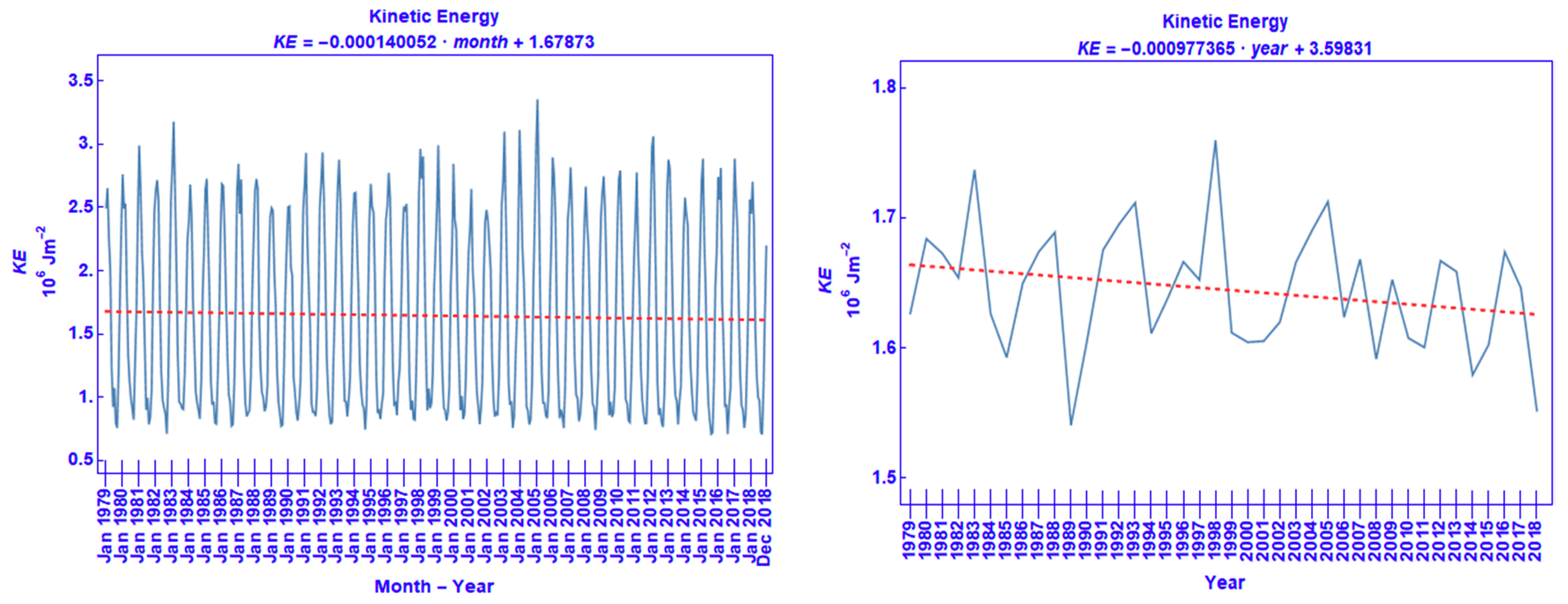
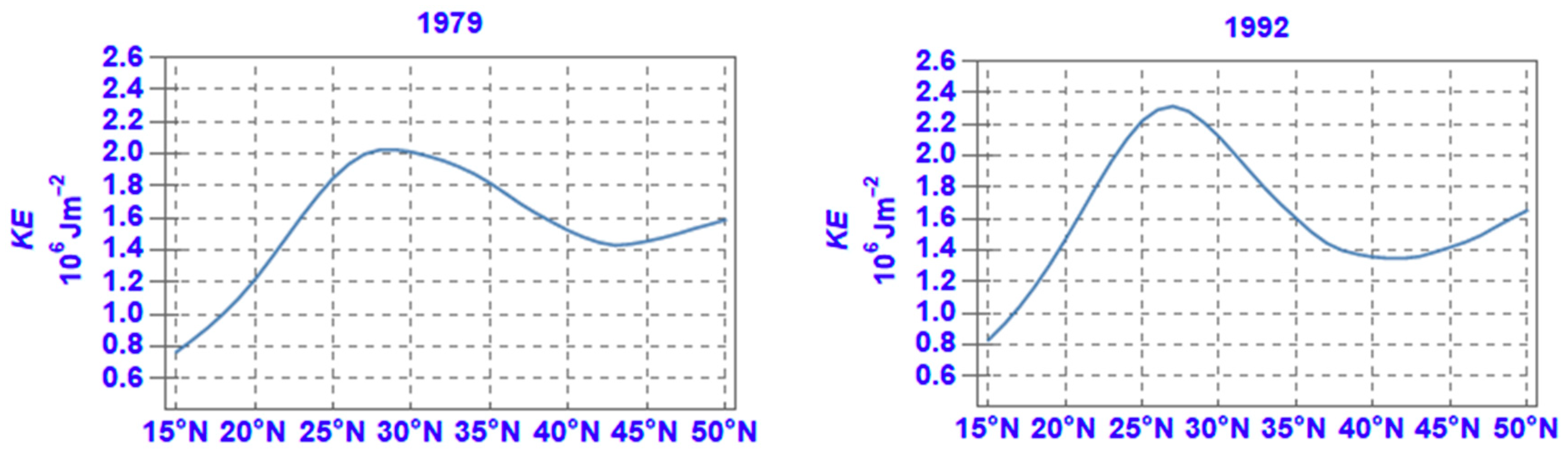
4.1. Kinetic Energy
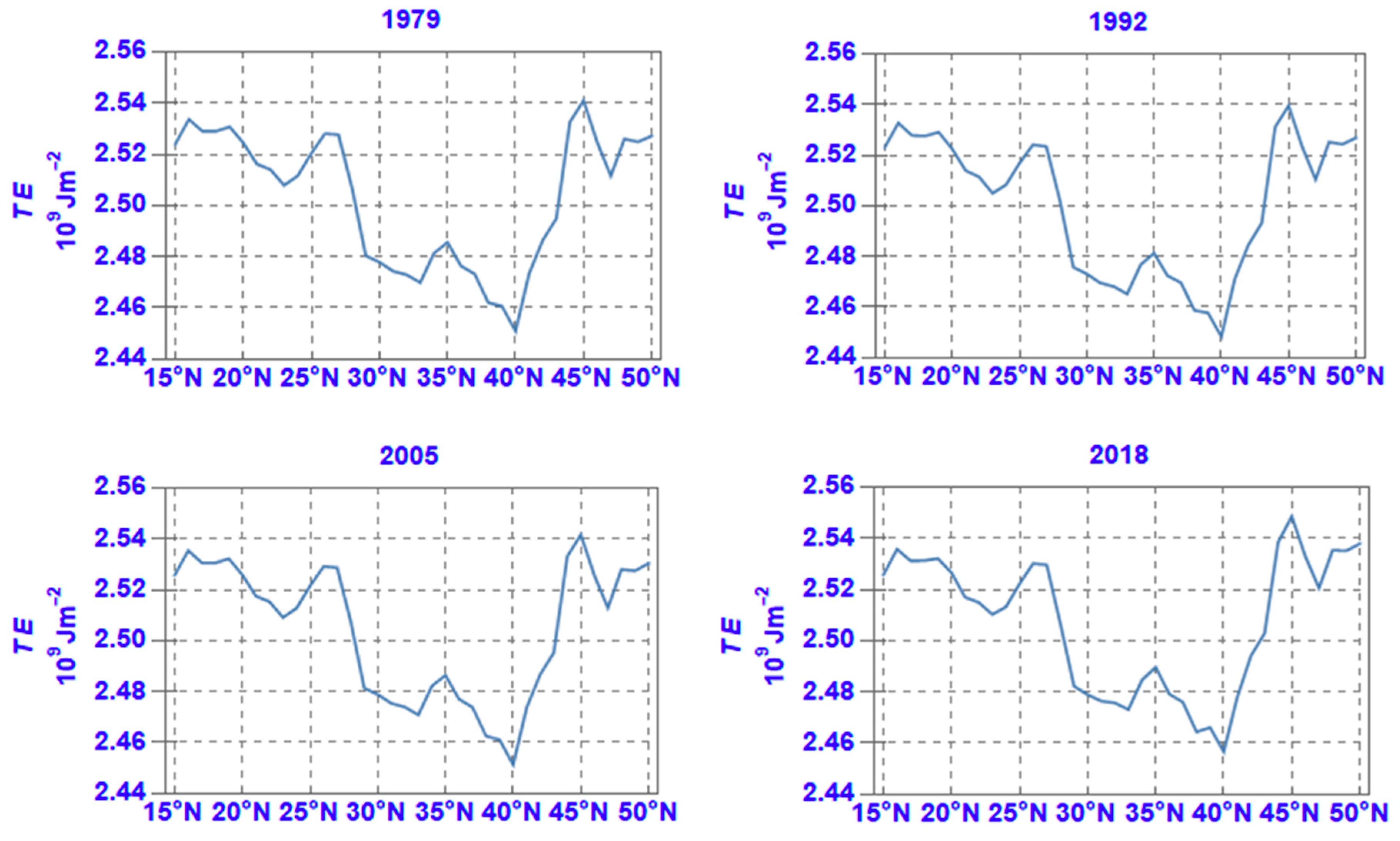
4.2. Thermal Energy
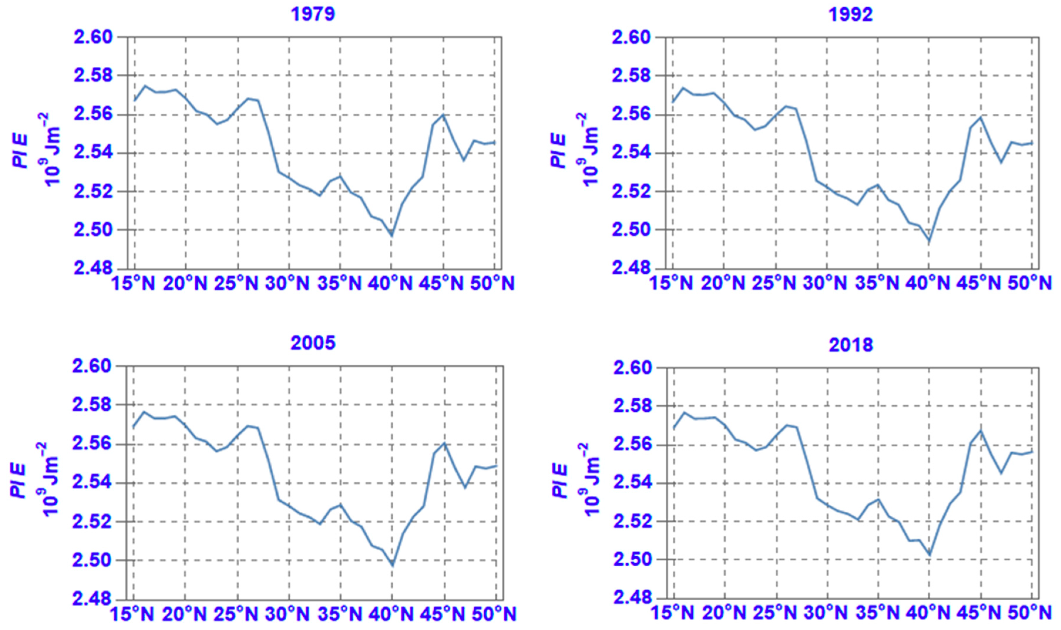
4.3. Potential Plus Internal Energy
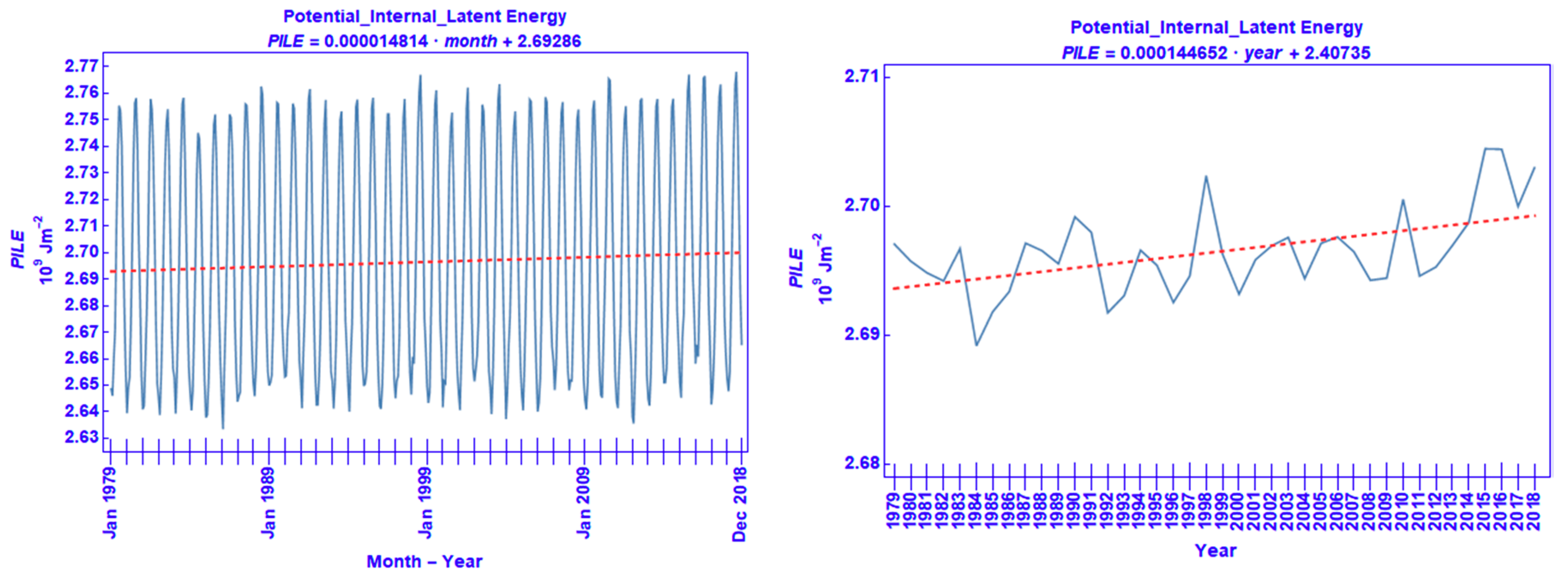
4.4. Potential, Internal Plus Latent Energies
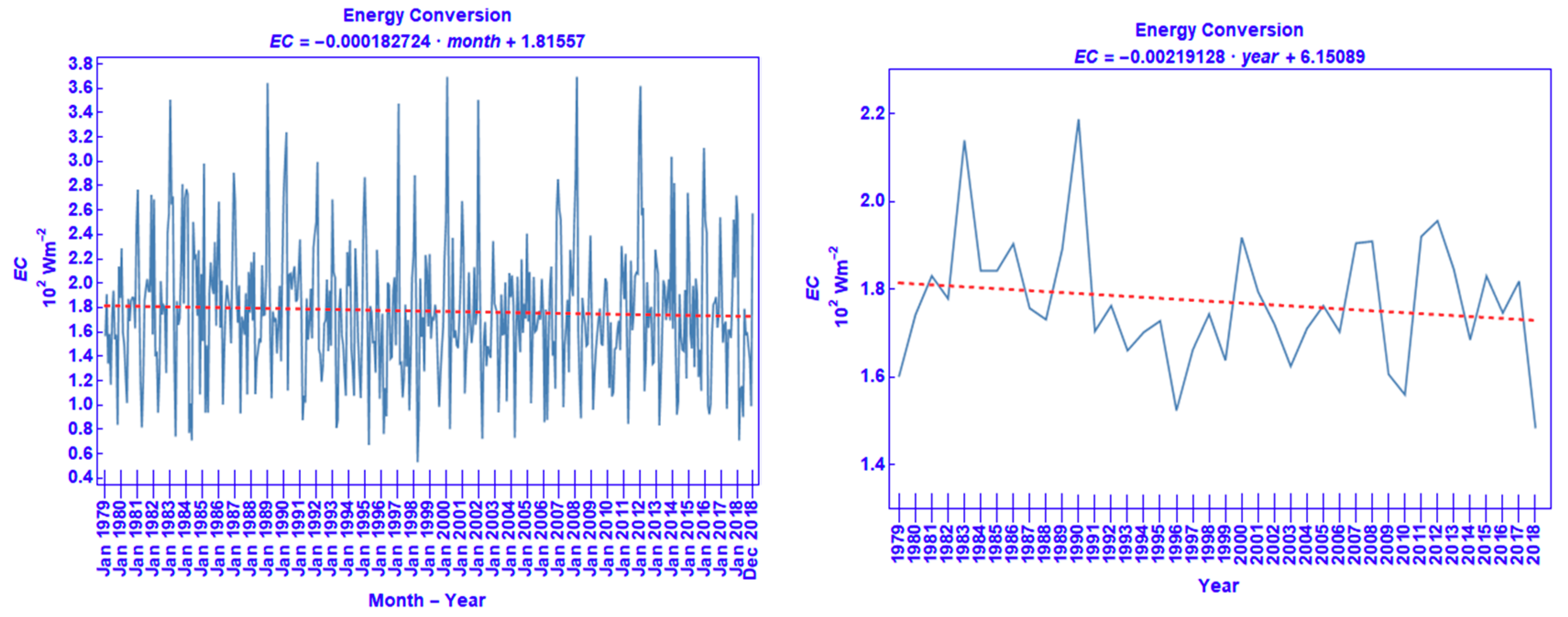
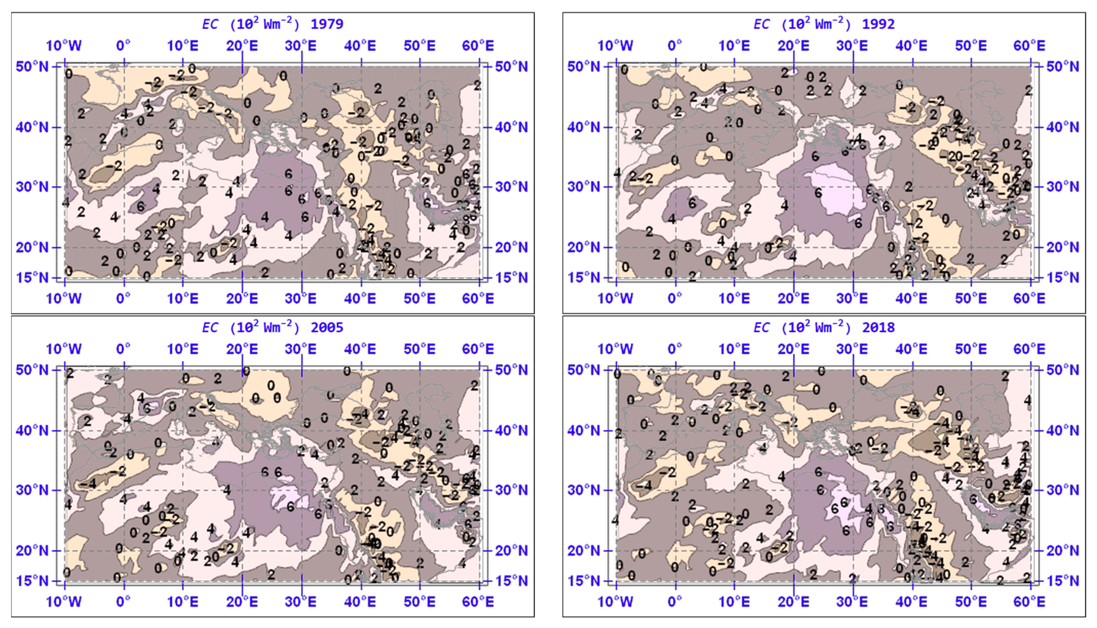
4.5. Energy Conversion
5. Discussion
6. Concluding Remarks
Supplementary Materials
Funding
Acknowledgments
Conflicts of Interest
Appendix A

| Symbol/Abbreviation | Explanation |
|---|---|
| Specific heat of (moist) air at constant pressure | |
| Specific heat of (moist) air at constant volume | |
| EC | Energy Conversion |
| g | Earth’s gravitational acceleration |
| IE | Internal Energy |
| KE | Kinetic Energy |
| L | Latent heat of evaporation = 2.5008 × 10⁶ J kg−1 |
| LE | Latent Energy |
| PE | Potential Energy |
| PIE | Potential + Internal Energy |
| PILE | Potential +Internal + Latent Energy |
| p | Pressure |
| ps | Surface pressure |
| q | Specific humidity |
| R | Gas constant for air |
| Τ | Temperature (in K) |
| t | Time |
| TE | Thermal Energy |
| Wind velocity vector | |
| η | Hybrid vertical coordinate |
| σ | =p/ps; Near-surface terrain following vertical coordinate |
| Geopotential | |
| Surface geopotential (or Orography) | |
| ω | =dp/dt; Pressure tendency (or Vertical velocity) |
| Zonal average of variable X | |
| Area average of variable X |
Appendix B
Appendix C
References
- Lelieveld, J.; Hadjinicolaou, P.; Kostopoulou, E.; Chenoweth, J.; Maayar, M.E.; Giannakopoulos, C.; Hannides, C.; Lange, M.A.; Tanarhte, M.; Tyrlis, E.; et al. Climate change and impacts in the Eastern Mediterranean and the Middle East. Clim. Chang. 2012, 114, 667–687. [Google Scholar] [CrossRef] [Green Version]
- Cook, B.I.; Anchukaitis, K.J.; Touchan, R.; Meko, D.M.; Cook, E.R. Spatiotemporal drought variability in the mediterranean over the last 900 years. J. Geophys. Res. 2016, 121, 2060–2074. [Google Scholar] [CrossRef] [PubMed]
- Bucchignani, E.; Mercogliano, P.; Panitz, H.J.; Montesarchio, M. Climate change projections for the Middle East–North Africa domain with COSMO-CLM at different spatial resolutions. Adv. Clim. Chang. Res. 2018, 9, 66–80. [Google Scholar] [CrossRef]
- Michaelides, S.C. Limited area energetics of Genoa cyclogenesis. Mon. Weather Rev. 1987, 13–26. [Google Scholar] [CrossRef]
- Michaelides, S.C. A spatial and temporal energetics anlysis of a baroclinic disturbance in the Mediterranean. Mon. Weather Rev. 1992, 120, 1224–1243. [Google Scholar] [CrossRef]
- Pan, Y.; Li, L.; Jiang, X.; Li, G.; Zhang, W.; Wang, X.; Ingersoll, A.P. Earth’s changing global atmospheric energy cycle in response to climate change. Nat. Commun. 2017, 8, 1–8. [Google Scholar] [CrossRef] [PubMed]
- Li, L.; Ingersoll, A.P.; Jiang, X.; Feldman, D.; Yung, Y.L. Lorenz energy cycle of the global atmosphere based on reanalysis datasets. Geophys. Res. Lett. 2007, 34, 1–5. [Google Scholar] [CrossRef] [Green Version]
- Prezerakos, N.G.; Michaelides, S.C. A composite diagnosis in sigma coordinates of the atmospheric energy balance during intense cyclonic activity. QJR. Meteorol. Soc. 1989, 115, 463–486. [Google Scholar] [CrossRef]
- Smith, P.J. On the contribution of a limited region to the global energy budget. Tellus 1969, 21, 202–207. [Google Scholar] [CrossRef] [Green Version]
- Smith, P.J.; Horn, L.H. A computational study of the energetics of a limited region of the atmosphere. Tellus 1969, 21, 193–201. [Google Scholar] [CrossRef] [Green Version]
- Berrisford, P.; Dee, D.; Fielding, K.; Fuentes, M.; Kallberg, P.; Kobayashi, S.; Uppala, S.; Simmons, A. The ERA-Interim Archive. Version 2.0. 2011. Available online: https://www.ecmwf.int/en/elibrary/8174-era-interim-archive-version-20 (accessed on 10 September 2020).
- Dee, D.P.; Uppala, S.M.; Simmons, A.J.; Berrisford, P.; Poli, P.; Kobayashi, S.; Andrae, U.; Balmaseda, M.A.; Balsamo, G.; Bauer, P.; et al. The ERA-Interim reanalysis: Configuration and performance of the data assimilation system. Q. J. R. Meteorol. Soc. 2011, 137, 553–597. [Google Scholar] [CrossRef]
- ECMWF. IFS Documentation CY31R1. 2007. Available online: https://www.ecmwf.int/en/publications/search/?solrsort=sort_labelasc&secondary_title=%22IFSDocumentationCY31R1%22 (accessed on 5 June 2020).
- Trenberth, K.E.; Caron, J.M.; Stepaniak, D.P. The atmospheric energy budget and implications for surface fluxes and ocean heat transports. Clim. Dyn. 2001, 17, 259–276. [Google Scholar] [CrossRef]
- Asiri, M.A.; Almazroui, M.; Awad, A.M. Synoptic features associated with the winter variability of the subtropical jet stream over Africa and the Middle East. Meteorol. Atmos. Phys. 2020. [Google Scholar] [CrossRef]
- Ljung, G.M.; Box, G.E.P. On a measure of lack of fit in time series models. Biometrika 1978, 65, 297–303. [Google Scholar] [CrossRef]
- Schütz, L.; Jaenicke, R.; Petrick, H. Saharan dust transport over the north Atlantic ocean. In Desert Dust: Origin, Characteristics and Effect on Man; Péwé, T.L., Ed.; Geological Society of America: Boulder, CO, USA, 1981; pp. 87–100. [Google Scholar]
- Kaufman, Y.J.; Tanré, D.; Boucher, O. A satellite view of aerosols in the climate system. Nature 2002, 419, 215–223. [Google Scholar] [CrossRef]
- Ben-Ami, Y.; Koren, I.; Altaratz, O.; Kostinski, A.; Lehahn, Y. Discernible rhythm in the spatio/temporal distributions of transatlantic dust. Atmos. Chem. Phys. 2012, 12, 2253–2262. [Google Scholar] [CrossRef] [Green Version]
- Haywood, J.M.; Allan, R.P.; Culverwell, I.; Slingo, T.; Milton, S.; Edwards, J.; Clerbaux, N. Can desert dust explain the outgoing longwave radiation anomaly over the Sahara during July 2003? J. Geophys. Res. D Atmos. 2005, 110, 1–14. [Google Scholar] [CrossRef]
- Miller, R.L.; Tegen, I. Climate response to soil dust aerosols. J. Clim. 1998, 11, 3247–3267. [Google Scholar] [CrossRef]
- Zhu, C.; Wang, B.; Qian, W. Why do dust storms decrease in northern China concurrently with the recent global warming? Geophys. Res. Lett. 2008, 35, 1–5. [Google Scholar] [CrossRef] [Green Version]
- Evan, A.T.; Flamant, C.; Gaetani, M.; Guichard, F. The past, present and future of African dust. Nature 2016, 531, 493–495. [Google Scholar] [CrossRef]
- Kok, J.F.; Ward, D.S.; Mahowald, N.M.; Evan, A.T. Global and regional importance of the direct dust-climate feedback. Nat. Commun. 2018, 9. [Google Scholar] [CrossRef] [PubMed]
- Kaufman, Y.J.; Tanré, D.; Dubovik, O.; Karnieli, A.; Remer, L.A. Absorption of sunlight by dust as inferred from satellite and ground-based remote sensing. Geophys. Res. Lett. 2001, 28, 1479–1482. [Google Scholar] [CrossRef] [Green Version]
- Granados-Muñoz, M.J.; Sicard, M.; Román, R.; Antonio Benavent-Oltra, J.; Barragán, R.; Brogniez, G.; Denjean, C.; Mallet, M.; Formenti, P.; Torres, B.; et al. Impact of mineral dust on shortwave and longwave radiation: Evaluation of different vertically resolved parameterizations in 1-D radiative transfer computations. Atmos. Chem. Phys. 2019, 19, 523–542. [Google Scholar] [CrossRef] [Green Version]
- Kishcha, P.; Alpert, P.; Barkan, J.; Kirschner, I.; Machenhauer, B. Atmospheric response to Saharan dust deduced from ECMWF reanalysis (ERA) temperature increments. Tellus B Chem. Phys. Meteorol. 2011, 55, 901–913. [Google Scholar] [CrossRef] [Green Version]
- Michaelides, S. Atmospheric energetics components over the Mediterranean, Middle East and North Africa for the period 1979–2017. In Proceedings of the 14th International Conference on Meteorology, Climatology and Atmospheric Physics (COMECAP 2018), Alexandroupoli, Greece, 15–17 October 2018; Kourtidis, K., Nastos, P., Moustris, K., Founda, D., Paschalidou, A., Eds.; Hellenic Meteorological Society: Athens, Greece, 2018; pp. 300–305, ISBN 978-960-98220-4-6. [Google Scholar]
- Margules, M. Über die Energie der Stürme (On the energy of storms-originally published by the Imperial Central Institute for Meteorology, Vienna, Austria, 1903; pp. 1–26). In The Mechanics of the Earth’s Atmosphere-A collection of Translations; Abbe, C., Ed.; English translation by Smithsonian Institution: Washington, WA, USA, 1904; Volume 51, pp. 533–595. [Google Scholar]
- Lorenz, E.N. Available Potential Energy and the Maintenance of the General Circulation. Tellus 1955, 7, 157–167. [Google Scholar] [CrossRef] [Green Version]
- Lorenz, E.N. The Nature and Theory of the General Circulation of the Atmosphere; World Meteorological Organization: Geneva, Switzerland, 1967. [Google Scholar]
- Lorenz, E.N. Energetics of atmospheric circulation. Int. Dict. Geophys. 1965, 66, 1–9. [Google Scholar]
- White, R.M.; Saltzman, B. On conversions between potential and kinetic energy in the atmosphere. Tellus 1956, 8, 357–363. [Google Scholar] [CrossRef] [Green Version]
- Mashat, A.W.S.; Awad, A.M.; Assiri, M.E.; Labban, A.H. Dynamic and synoptic study of spring dust storms over northern Saudi Arabia. Theor. Appl. Climatol. 2020, 140, 619–634. [Google Scholar] [CrossRef]
- Trenberth, K.E. Climate diagnostics from global analyses: Climate diagnostics from global analyses: Conservation of mass in ECMWF analyses. J. Clim. 1991, 4, 707–722. [Google Scholar] [CrossRef] [Green Version]
- Trenberth, K.E. Using atmospheric budgets as a constraint on surface fluxes. J. Clim. 1997, 10, 2796–2809. [Google Scholar] [CrossRef]
- Trenberth, K.E.; Fasullo, J.T. Applications of an updated atmospheric energetics formulation. J. Clim. 1991, 31, 6263–6279. [Google Scholar] [CrossRef]
- Trenberth, K.E.; Stepaniak, D.P.; Caron, J.M. Accuracy of atmospheric energy budgets from analyses. J. Clim. 2002, 15, 3343–3360. [Google Scholar] [CrossRef]


© 2020 by the author. Licensee MDPI, Basel, Switzerland. This article is an open access article distributed under the terms and conditions of the Creative Commons Attribution (CC BY) license (http://creativecommons.org/licenses/by/4.0/).
Share and Cite
Michaelides, S. Long-Term Analysis of Atmospheric Energetics Components over the Mediterranean, Middle East and North Africa. Atmosphere 2020, 11, 976. https://doi.org/10.3390/atmos11090976
Michaelides S. Long-Term Analysis of Atmospheric Energetics Components over the Mediterranean, Middle East and North Africa. Atmosphere. 2020; 11(9):976. https://doi.org/10.3390/atmos11090976
Chicago/Turabian StyleMichaelides, Silas. 2020. "Long-Term Analysis of Atmospheric Energetics Components over the Mediterranean, Middle East and North Africa" Atmosphere 11, no. 9: 976. https://doi.org/10.3390/atmos11090976