Monitoring of Gas Emissions in Light of an OEF Application


 ,
,
Abstract
1. Introduction
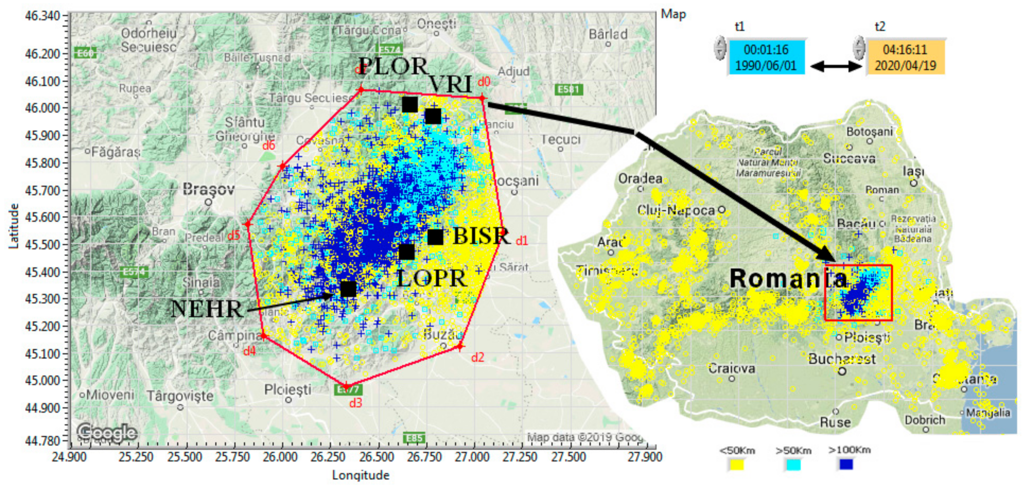
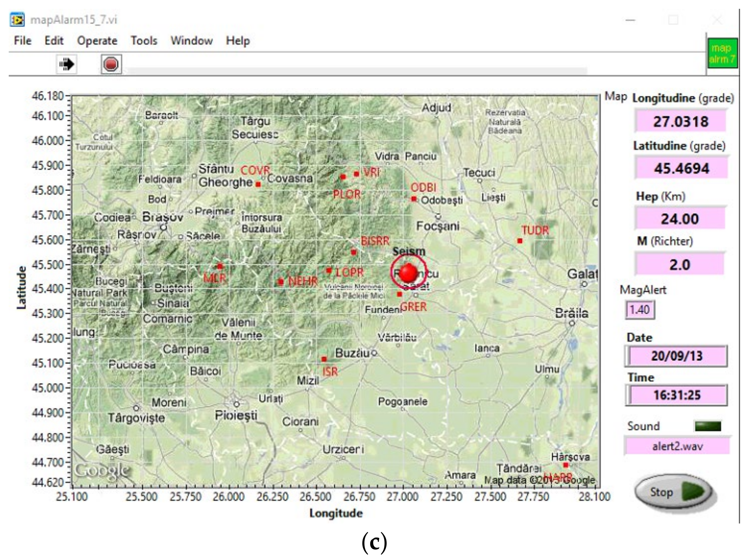
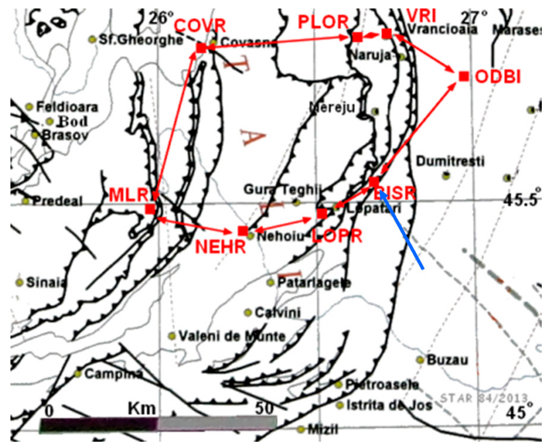
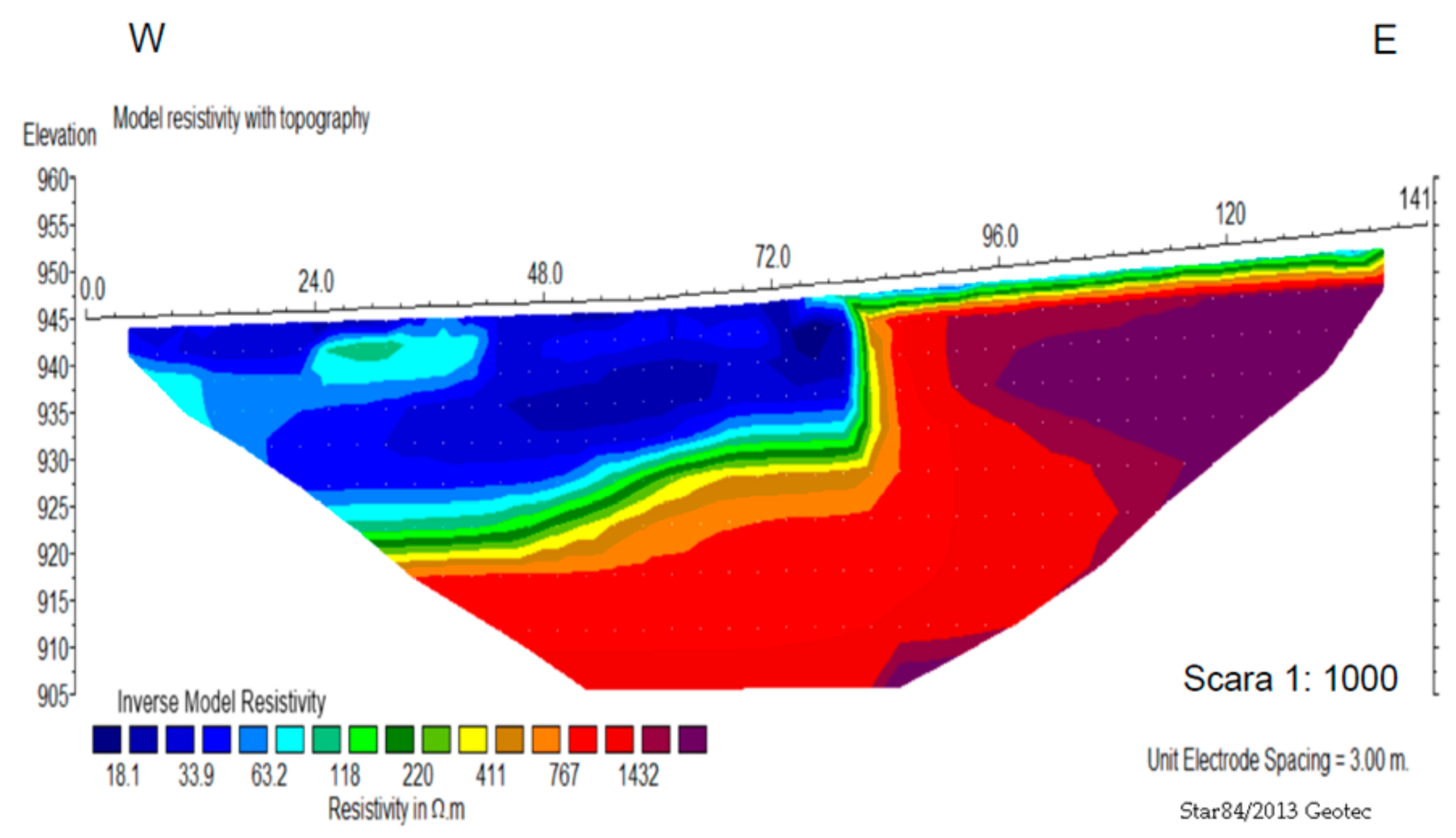
2. Monitoring Network
3. Data, Methods, Procedure
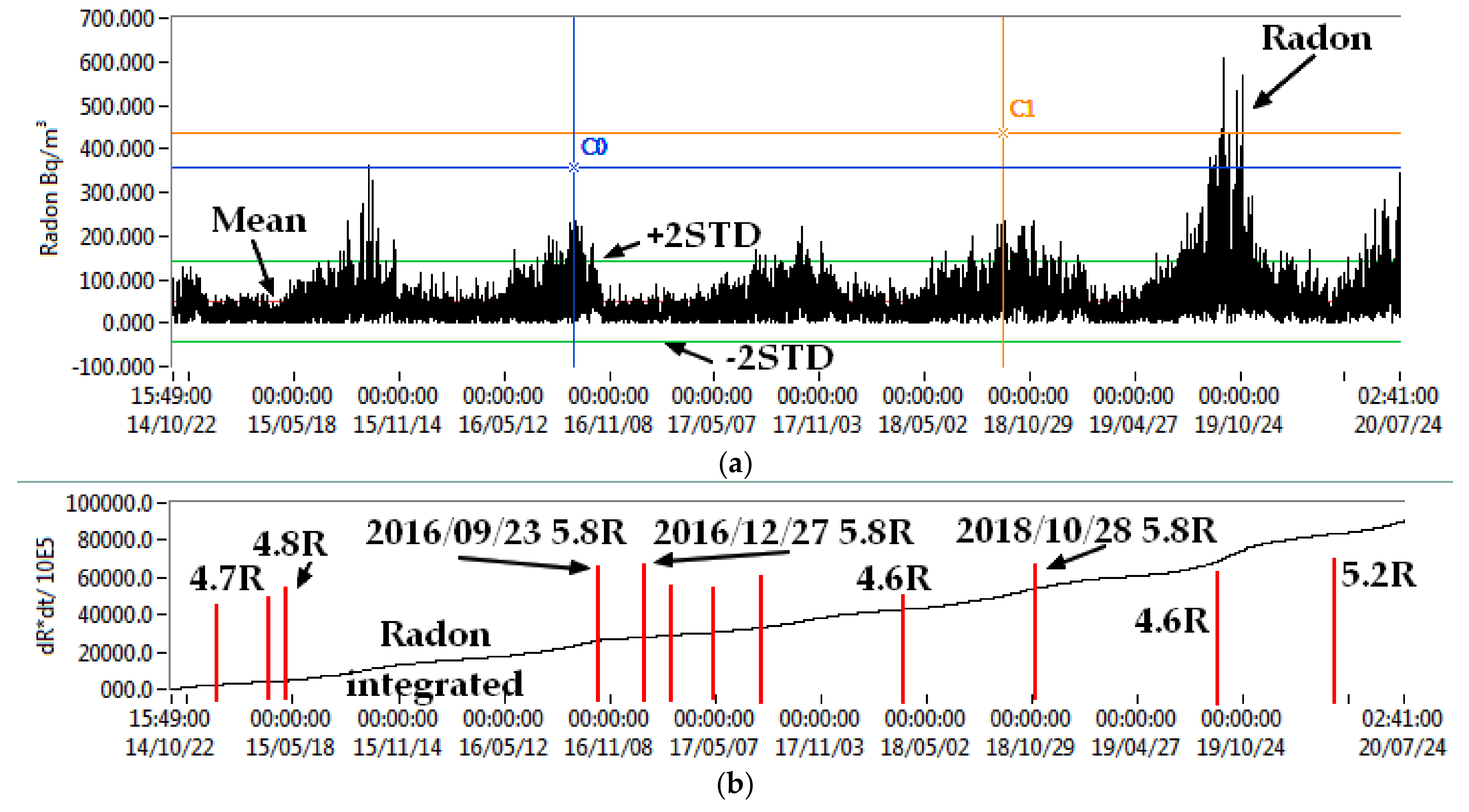
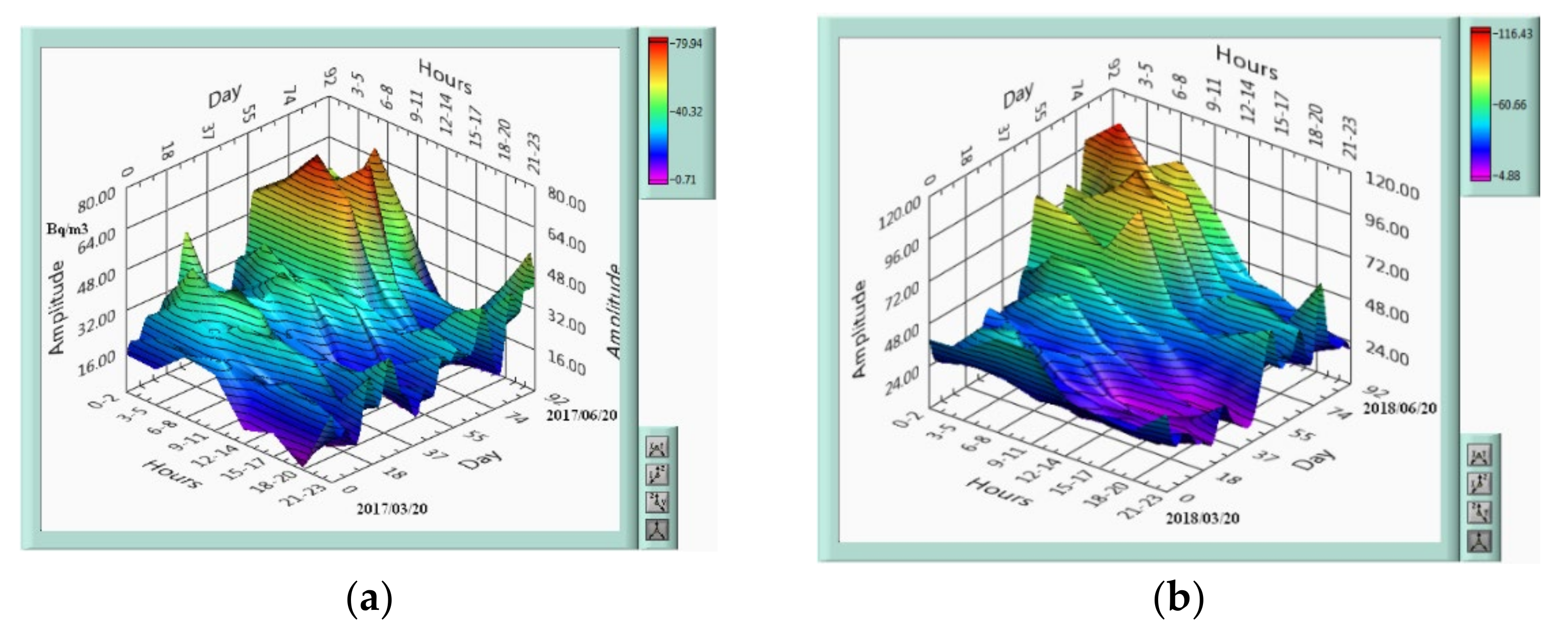
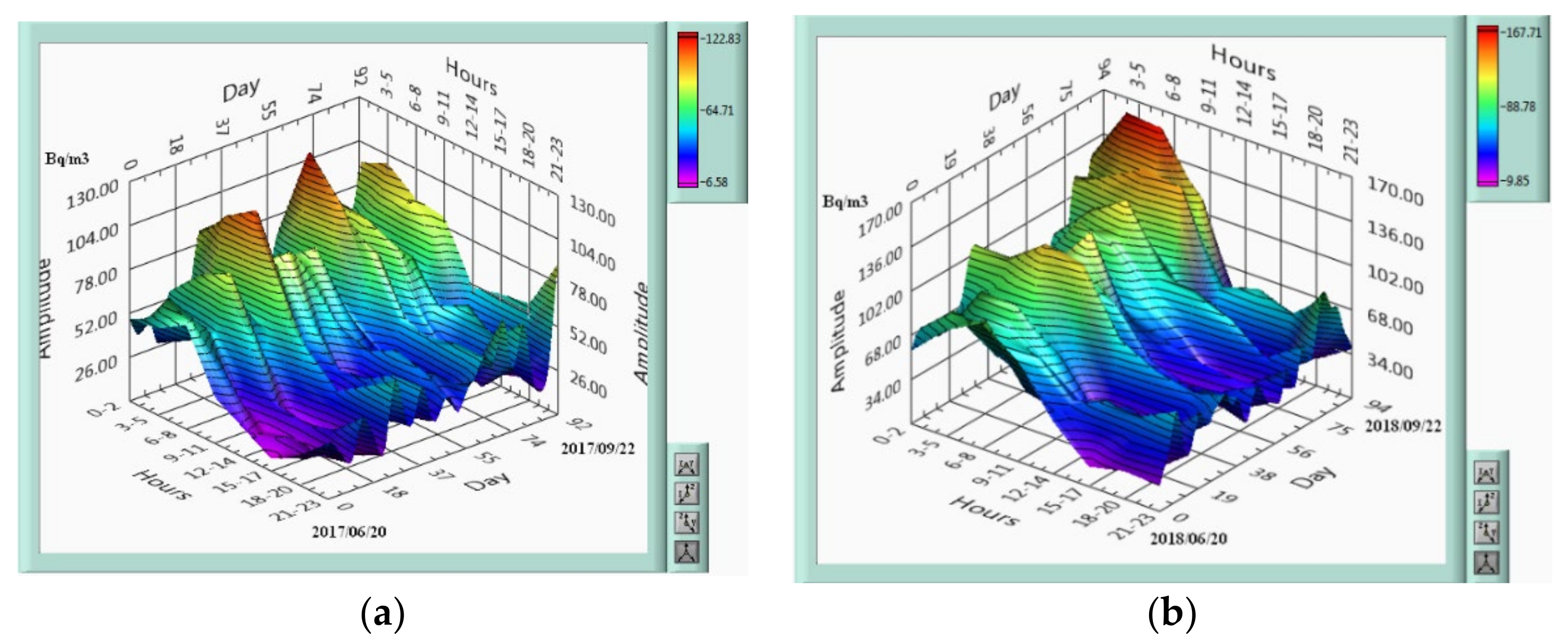
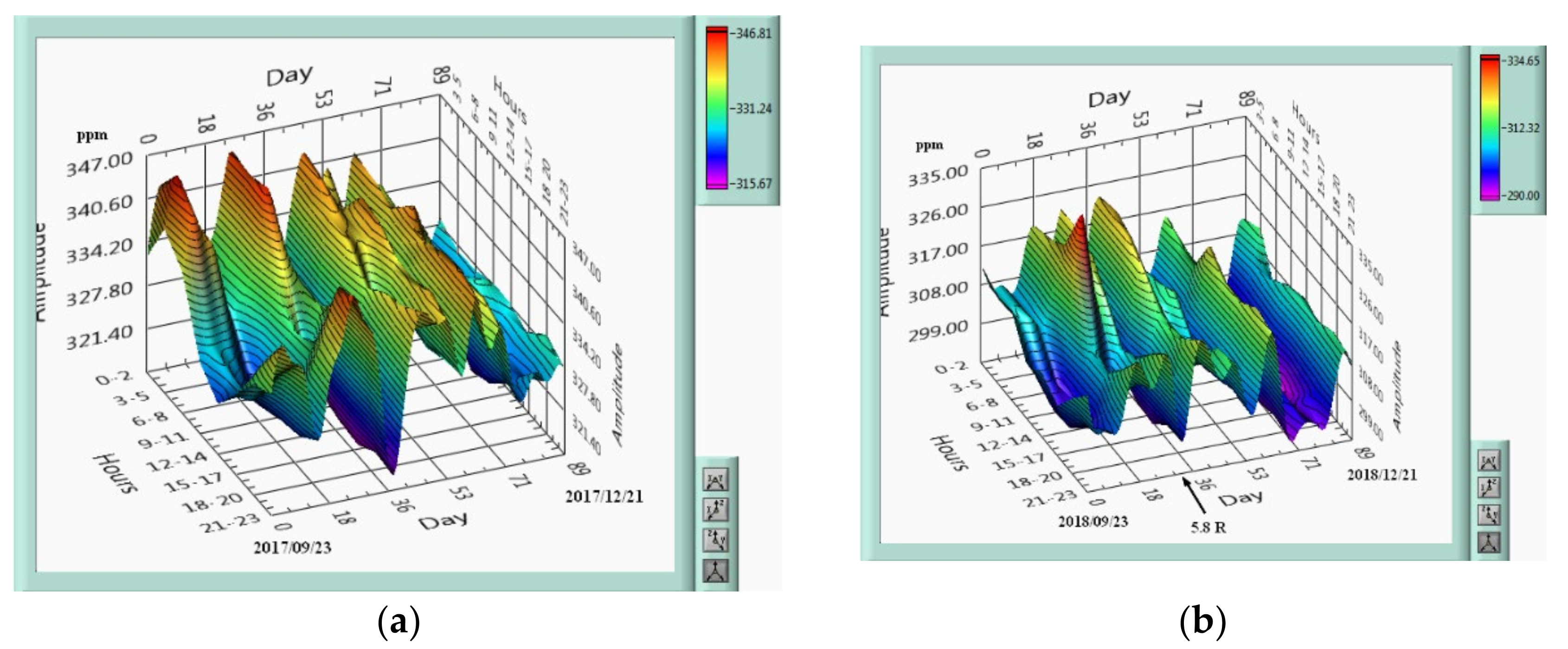
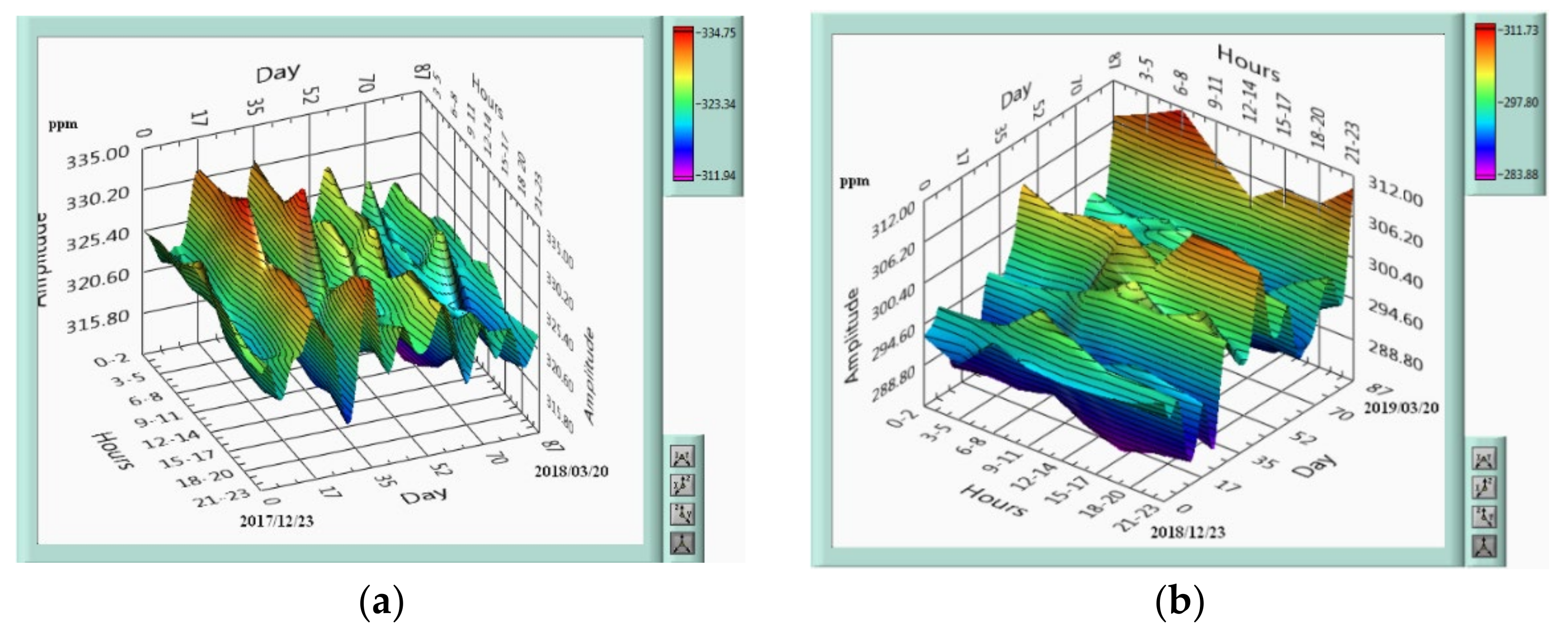
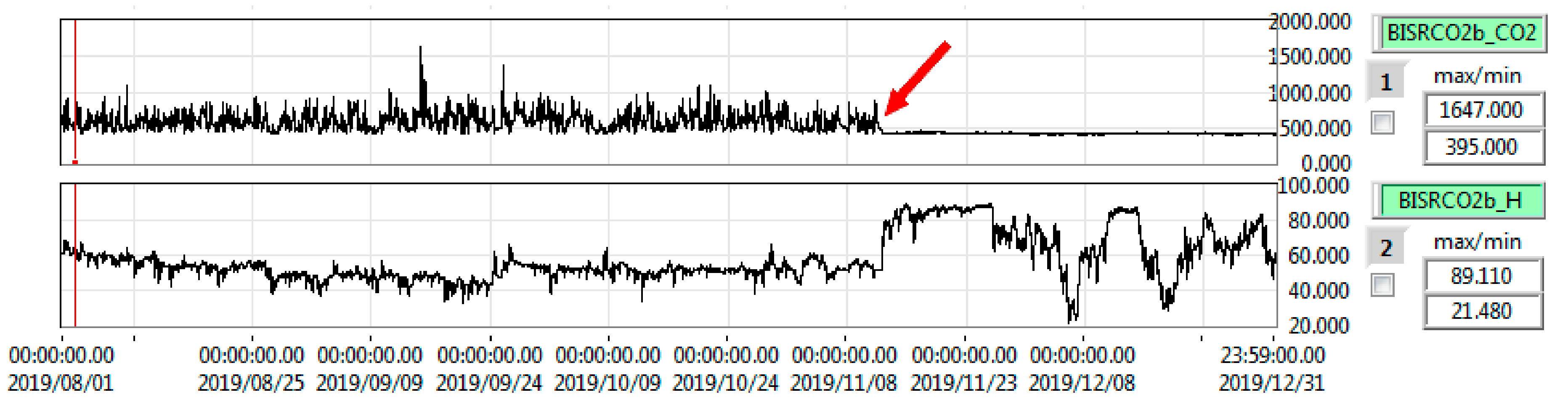
3.1. Data and Detection Methods
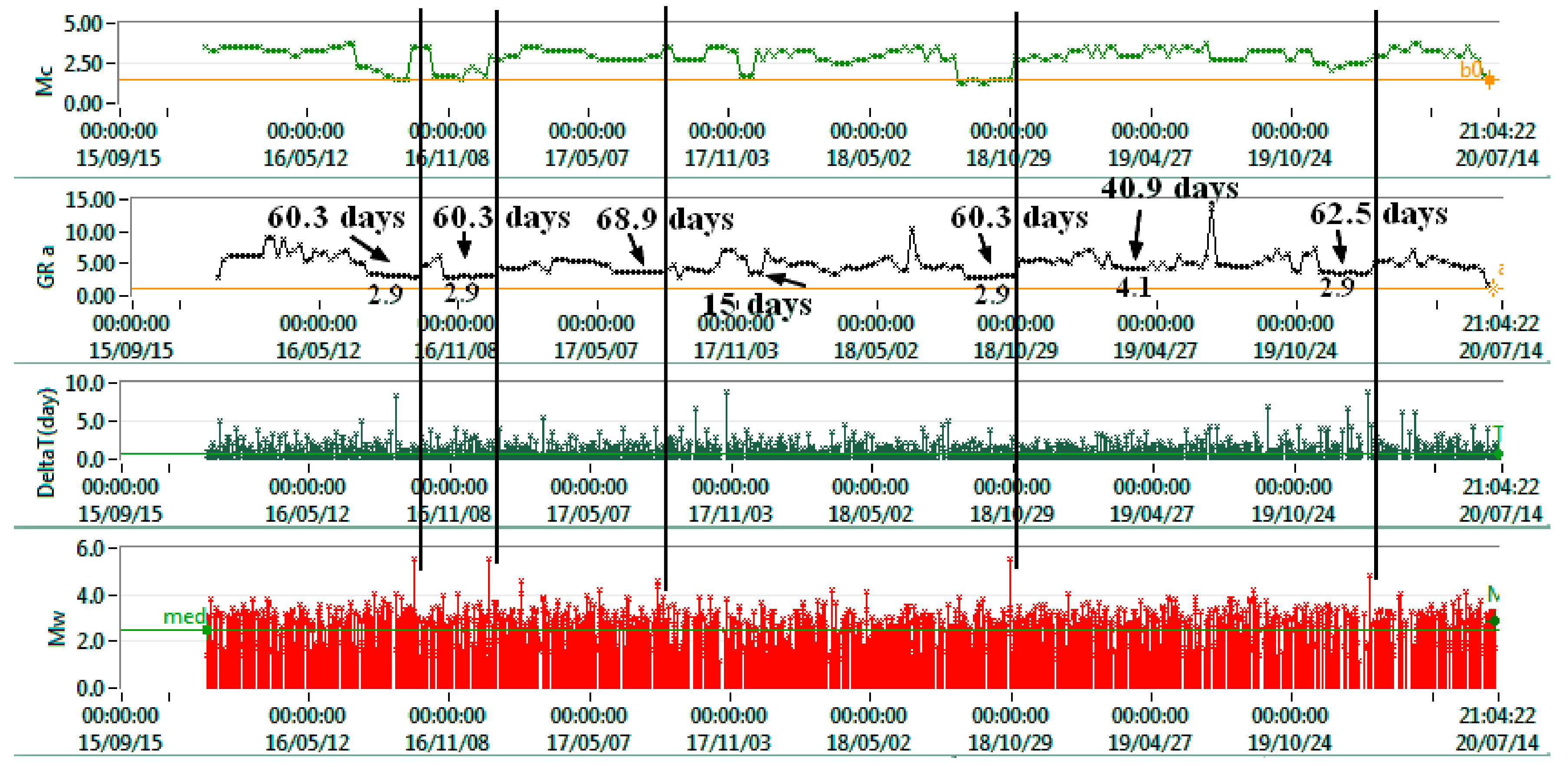
3.2. OEF Procedure
- <?xml version=“1.0” encoding=“UTF-8” standalone=“yes”?>
- <data-set xmlns:xsi=“http://www.w3.org/2001/XMLSchema-instance”>
- <record>
- <Type>Radon</Type>
- <Station>BISRd</Station>
- <Probability>0.57</Probability>
- <Uncertain>4.98</Uncertain>
- <Weight>0.18</Weight>
- </record>
- <record>
- <Type>Radon</Type>
- <Station>LOPRd</Station>
- <Probability>0.29</Probability>
- <Uncertain>3.93</Uncertain>
- <Weight>0.14</Weight>
- </record> …
4. Discussion and Conclusions
Author Contributions
Funding
Institutional Review Board Statement
Informed Consent Statement
Data Availability Statement
Acknowledgments
Conflicts of Interest
References
- Pulinets, S. The Possibility of Earthquake Forecasting: Learning from Nature; Institute of Physics Publishing (Great Britain): Bristol, UK, 2018; Volume 16, ISBN 978-0-7503-1248-6. [Google Scholar]
- Cannelli, V.; Piersanti, A.; Galli, G.; Melini, D. Italian radon monitoring network (Iron): A permanent network for near real-time monitoring of soil radon emission in Italy. Ann. Geophys. 2018, 61, 1–22. [Google Scholar] [CrossRef]
- Piersanti, A.; Cannelli, V.; Galli, G. Long term continuous radon monitoring in a seismically active area. Ann. Geophys. 2015, 58. [Google Scholar] [CrossRef]
- Morita, M.; Mori, T.; Yokoo, A.; Ohkura, T.; Morita, Y. Continuous monitoring of soil CO2 flux at Aso volcano, Japan: The influence of environmental parameters on diffuse degassing. Earth Planets Space 2019, 71, 1. [Google Scholar] [CrossRef]
- Castellana, L.; Biagi, P.F. Detection of hydrogeochemical seismic precursors by a statistical learning model. Nat. Hazards Earth Syst. Sci. 2008, 8, 1207–1216. [Google Scholar] [CrossRef]
- Foulser-Piggott, R.; Bowman, G.; Hughes, M. A Framework for Understanding Uncertainty in Seismic Risk Assessment. Risk Anal. 2020, 40, 169–182. [Google Scholar] [CrossRef]
- Yuce, G.; Ugurluoglu, D.Y.; Adar, N.; Yalcin, T.; Yaltirak, C.; Streil, T.; Oeser, V. Monitoring of earthquake precursors by multi-parameter stations in Eskisehir region (Turkey). Appl. Geochem. 2010, 25, 572–579. [Google Scholar] [CrossRef]
- Werner, C.; Cardellini, C. Comparison of carbon dioxide emissions with fluid upflow, chemistry, and geologic structures at the Rotorua geothermal system, New Zealand. Geothermics 2006, 35, 221–238. [Google Scholar] [CrossRef]
- Weinlich, F.H. Carbon dioxide controlled earthquake distribution pattern in the NW Bohemian swarm earthquake region, western Eger Rift, Czech Republic–gas migration in the crystalline basement. Geofluids 2014, 14, 143–159. [Google Scholar] [CrossRef]
- Chiodini, G.; Cardellini, C.; Amato, A.; Boschi, E.; Caliro, S.; Frondini, F.; Ventura, G. Carbon dioxide Earth degassing and seismogenesis in central and southern Italy. Geophys. Res. Lett. 2004, 31, 2–5. [Google Scholar] [CrossRef]
- Okumura, S.; Hirano, N. Carbon dioxide emission to earth’s surface by deep-sea volcanism. Geology 2013, 41, 1167–1170. [Google Scholar] [CrossRef]
- Chiodini, G.; Cardellini, C.; Lamberti, M.C.; Agusto, M.; Caselli, A.; Liccioli, C.; Tamburello, G.; Tassi, F.; Vaselli, O.; Caliro, S. Carbon dioxide diffuse emission and thermal energy release from hydrothermal systems at Copahue-Caviahue Volcanic Complex (Argentina). J. Volcanol. Geotherm. Res. 2015, 304, 294–303. [Google Scholar] [CrossRef]
- Ármannsson, H. An overview of carbon dioxide emissions from Icelandic geothermal areas. Procedia Earth Planet. Sci. 2017, 97, 11–18. [Google Scholar] [CrossRef]
- Ármannsson, H. Carbon Dioxide Emissions from Icelandic Geothermal Areas. Procedia Earth Planet. Sci. 2017, 17, 104–107. [Google Scholar] [CrossRef]
- Fridriksson, T.; Kristjánsson, B.R.; Ármannsson, H.; Margrétardóttir, E.; Ólafsdóttir, S.; Chiodini, G. CO2 emissions and heat flow through soil, fumaroles, and steam heated mud pools at the Reykjanes geothermal area, SW Iceland. Appl. Geochem. 2006, 21, 1551–1569. [Google Scholar] [CrossRef]
- Heinicke, J.; Koch, U.; Martinelli, G. CO2 and Radon measurements in the Vogtland area (Germany)—A contribution to earthquqke prediction research. Geophys. Res. Lett. 1995, 22, 771–774. [Google Scholar] [CrossRef]
- Jilani, Z.; Mehmood, T.; Alam, A.; Awais Muhammadand Iqbal, T. Monitoring and descriptive analysis of radon in relation to seismicactivity of Northern Pakistan. J. Environ. Radioact. 2017, 172, 43–51. [Google Scholar] [CrossRef]
- Famin, V.; Nakashima, S.; Boullier, A.M.; Fujimoto, K.; Hirono, T. Earthquakes produce carbon dioxide in crustal faults. Earth Planet. Sci. Lett. 2008, 265, 487–497. [Google Scholar] [CrossRef]
- Sugisaki, R.; Anno, H.; Adachi, M.; Ui, H. Geochemical features of gases and rocks along active faults. Geochem. J. 1980, 14, 101–112. [Google Scholar] [CrossRef]
- Frunzeti, N.; Baciu, C.; Etiope, G.; Pfanz, H. Geogenic emission of methane and carbon dioxide at Beciu mud volcano, (Berca-Arbǎnaşi hydrocarbon-bearing structure, Eastern Carpathians, Romania). Carpath. J. Earth Environ. Sci. 2012, 7, 159–166. [Google Scholar] [CrossRef]
- Martinelli, G.; Albarello, D.; Mucciarelli, M. Radon Emissions from Mud Volcanos in Northern Italy–Possible Connection with Local Seismicity. Geophys. Res. Lett. 1995, 22, 1989–1992. [Google Scholar] [CrossRef]
- Etiope, G.; Baciu, C.; Caracausi, A.; Italiano, F.; Cosma, C. Gas flux to the atmosphere from mud volcanoes in eastern Romania. Terra Nov. 2004, 16, 179–184. [Google Scholar] [CrossRef]
- Nevinsky, V.; Nevinsky, I.; Tsvetkova, T. Measurements of soil radon in south Russia for seismologicalapplication: Methodological aspects. Radiat. Meas. 2012, 47, 281–291. [Google Scholar] [CrossRef]
- Brustur, T.; Stănescu, I.; Macaleţ, R.; Melinte-Dobrinescu, M.C. The mud volcanoes from Berca: A significant geological patrimony site of the BuzĂu Land Geopark (Romania). GeoEcoMarina 2015, 2015, 73–96. [Google Scholar] [CrossRef]
- Zoran, M.; Savastru, R.; Savastru, D. Radon levels assessment in relation with seismic events in Vrancea region. J. Radioanal. Nucl. Chem. 2012, 293, 655–663. [Google Scholar] [CrossRef]
- Woo, G.; Marzocchi, W. Operational Earthquake Forecasting and Decision-Making. In Early Warning for Geological Disasters; Springer: Berlin/Heidelberg, Germany, 2014; Volume 81, pp. 353–367. ISBN 978-3-642-12232-3. [Google Scholar]
- Jordan, T.H.; Jordan, T.H.; Chen, Y.-T.T.; Gasparini, P.; Madariaga, R.; Main, I.; Marzocchi, W.; Papadopoulos, G.; Sobolev, G.; Yamaoka, K.; et al. Operational earthquake forecasting: State of knowledge and guidelines for utilization. Ann. Geophys. 2011, 54, 319–391. [Google Scholar] [CrossRef]
- Trnkoczy, A. Understanding and parameter setting of STA/LTA trigger algorithm. New Man. Seismol. Obs. Pract. 2012, 20. [Google Scholar] [CrossRef]
- Baillard, C.; Crawford, W.C.; Ballu, V.; Hibert, C.; Mangeney, A. An automatic kurtosis-based P-and S-phase picker designed for local seismic networks. Bull. Seismol. Soc. Am. 2014, 104, 394–409. [Google Scholar] [CrossRef]
- Agletdinov, E.; Merson, D.; Vinogradov, A. A new method of low amplitude signal detection and its application in acoustic emission. Appl. Sci. 2020, 10, 73. [Google Scholar] [CrossRef]
- Vassallo, M.; Satriano, C.; Lomax, A. Automatic picker developments and optimization: A strategy for improving the performances of automatic phase pickers. Seismol. Res. Lett. 2012, 83, 541–554. [Google Scholar] [CrossRef]
- Banfill Software Engineering. Available online: https://banfill.net/?page_id=16,Banfill (accessed on 15 September 2020).
- Trnkoczy, A. Understanding and Setting STA/LTA Trigger Algorithm Parameters for the K2. Appl Note 1998, 41, 16–20. [Google Scholar]
- Allen, R. Automatic phase pickers: Their present use and future prospects. Bull. Seismol. Soc. Am. 1982, 72, S225–S242. [Google Scholar]
- Chi-Durán, R.; Comte, D.; Díaz, M.; Silva, J.F. Automatic detection of P- and S-wave arrival times: New strategies based on the modified fractal method and basic matching pursuit. J. Seismol. 2017, 21, 1171–1184. [Google Scholar] [CrossRef]
- Gregori, A.; Zmazek, B.; Deroski, S.; Torkar, D.; Vaupoti, J. Radon as an Earthquake Precursor—Methods for Detecting Anomalies. In Earthquake Research and Analysis—Statistical Studies, Observations and Planning; IntechOpen: London, UK, 2012; pp. 179–196. ISBN 978-953-51-0134-5. [Google Scholar] [CrossRef]
- Kijko, A. Estimation of Gutenberg-Richter b-value without Level of Completeness Apparent (Observed) Frequency-Magnitude Distribution Proposed Parametrization. Annu. Meet. SSA 2016, 19–20. [Google Scholar] [CrossRef]
- Utsu, T. A method for determining the value of b in a formula logN=a-bM showing the magnitude-frequency relation for earthquakes. Geophys. Bull. Hokkaido Univ. 1965, 13, 99–103. [Google Scholar] [CrossRef]
- Enescu, B.; Enescu, D.; Ito, K. Values of b and p: Their variations and relation to physical processes for earthquakes in Japan and Romania. Rom. Rep. Phys. 2011, 56, 590–608. [Google Scholar]
- Bilim, F. The correlation of b-value in the earthquake frequency-magnitude distribution, heat flow and gravity data in the Sivas Basin, central eastern Turkey. Bitlis Eren Univ. J. Sci. Technol. 2019, 9, 11–15. [Google Scholar] [CrossRef][Green Version]
- Gutenberg, B.; Richter, C.F. Earthquake magnitude, intensity, energy, and acceleration: (Second paper). Bull. Seismol. Soc. Am. 1956, 46, 105–145. [Google Scholar]
- Dobrovolsky, I.P.; Zubkov, S.I.; Miachkin, V.I. Estimation of the size of earthquake preparation zones. Pure Appl. Geophys. Pageoph 1979, 117, 1025–1044. [Google Scholar] [CrossRef]
- Tchorz-Trzeciakiewicz, D.E.; Solecki, A.T. Seasonal variation of radon concentrations in atmospheric air in the Nowa Ruda area (Sudety Mountains) of southwest Poland. Geochem. J. 2011, 45, 455–461. [Google Scholar] [CrossRef]
- Süer, S.; Wiersberg, T.; Güleç, N.; Erzinger, J.; Parlaktuna, M. Geochemical Monitoring of the Seismic Activities and Noble Gas Characterization of the Geothermal Fields along the Eastern Segment of the Büyük Menderes Graben SETTING AND RECENT. In Proceedings of the World Geothermal Congress, Bali, Indonesia, 25–30 April 2010; pp. 25–29. [Google Scholar]
- Ridler, N.; Lee, B.; Martens, J.; Wong, K. Measurement uncertainty, traceability, and the GUM. IEEE Microw. Mag. 2007, 8, 44–53. [Google Scholar] [CrossRef]
- Kitov, I.O.; Sanina, I.A.; Sergeev, S.S.; Nesterkina, M.A.; Konstantinovskaya, N.L. Detection, Estimation of Magnitude, and Relative Location of Weak Aftershocks Using Waveform Cross-Correlation: The Earthquake of August 7, 2016, in the Town of Mariupol. Seism. Instrum. 2018, 54, 158–174. [Google Scholar] [CrossRef]
- Rusov, V.D.; Maksymchuk, V.Y.; Ilić, R.; Pavlovych, V.M.; Bakhmutov, V.G.; Saranuk, D.N.; Vaschenko, V.M.; Skvarč, J.; Hanžič, L.; Rusov, V.D.; et al. The Peculiarities of Cross-Correlation between Two Secondary Precursors—Radon and Magnetic Field Variations, Induced by Tectonic Activity V.D. Ukr. Antarct. J. 2006, 160–181. [Google Scholar] [CrossRef]
- Vaughan, N.; Lenton, T. Interactions between reducing CO2 emissions, CO2 removal and solar radiation management. Philos. Trans. R. Soc. A Math. Phys. Eng. Sci. 2012, 370, 4343–4364. [Google Scholar] [CrossRef] [PubMed]
- Toader, V.E.E.; Biagi, P.F.; Moldovan, I. Evaluation of the Solar Radiation in a Seismic Zone. IOP Conf. Ser. Earth Environ. Sci. 2019, 362, 012069. [Google Scholar] [CrossRef]
- Bommer, J.J. On the Use of Logic Trees for Ground-Motion Prediction Equations in Seismic-Hazard Analysis. Bull. Seismol. Soc. Am. 2005, 95, 377–389. [Google Scholar] [CrossRef]
- Grünthal, G.; Stromeyer, D.; Bosse, C.; Cotton, F.; Bindi, D. The probabilistic seismic hazard assessment of Germany—Version 2016, considering the range of epistemic uncertainties and aleatory variability. Bull. Earthq. Eng. 2018, 16, 4339–4395. [Google Scholar] [CrossRef]
- Molina, S.; Lang, D.H.; Lindholm, C.D. SELENA—An open-source tool for seismic risk and loss assessment using a logic tree computation procedure. Comput. Geosci. 2010, 36, 257–269. [Google Scholar] [CrossRef]
- Hauser, F.; Raileanu, V.; Fielitz, W.; Bala, A.; Prodehl, C.; Polonic, G.; Schulze, A. VRANCEA99-The crustal structure beneath the Southeastern Carpathians and the Moesian platform from a seismic refraction profile in Romania. Tectonophysics 2001, 340, 233–256. [Google Scholar] [CrossRef]
- Kastelis, N.; Kourtidis, K. Characteristics of the atmospheric electric field and correlation with CO2 at a rural site in southern Balkans. Earth Planets Space 2016, 68, 1–15. [Google Scholar] [CrossRef]
- Abbad, S.; Robe, M.C.; Bernat, M.; Labed, V. Influence of meteorological and geological parameter variables on the concentration of radon in soil gases: Application to seismic forecasting in the Provence-Alpes-Cote d’Azur region. Environ. Geochem. Health 1995, 16, 35–48. [Google Scholar]
- Lane-Smith, D.; Sims, K.W.W. The effect of CO2 on the measurement of 220Rn and 222Rn with instruments utilising electrostatic precipitation. Acta Geophys. 2013, 61, 822–830. [Google Scholar] [CrossRef]
- Mihai, A.; Moldovan, I.A.; Toader, V.E.; Petrescu, L.; Partheniu, R. Geomagnetic Field Behaviour at Muntele Rosu (Romania) and Anomaly Interpretation. IOP Conf. Ser. Earth Environ. Sci. 2019, 221, 1–10. [Google Scholar] [CrossRef]
- Zechar, J.D.; Marzocchi, W.; Wiemer, S. Operational earthquake forecasting in Europe: Progress, despite challenges. Bull. Earthq. Eng. 2016, 14, 2459–2469. [Google Scholar] [CrossRef]


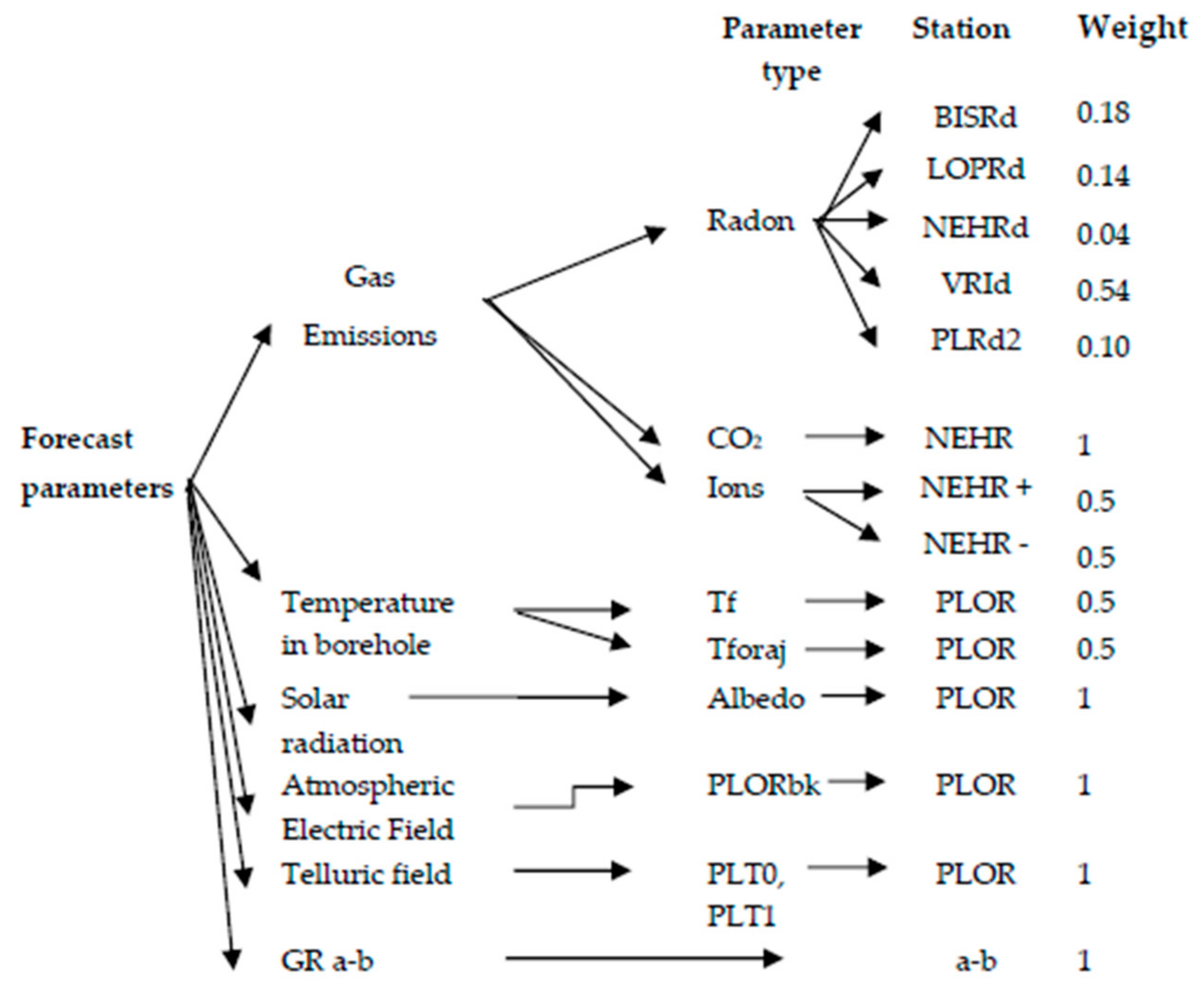
| Station Name Lat/Lon | Code | Equipment | Sampling Period |
|---|---|---|---|
| Bisoca BISR 45.5481l/26.7099 | BISRd | Radon equipment with inclinometer, air temperature, pressure and humidity | 3 h |
| BISRCO2 | CO2, CO, air temperature, humidity, and meteorological station | 1 s | |
| Lopatari LOPR 45.4738/26.568 | LOPRd | Radon equipment with inclinometer, air temperature, pressure and humidity | 3 h |
| LOPrCO2 | CO2, CO, air temperature, humidity | 1 s | |
| Nehoiu NEHR 45.4272/26.2952 | NEHRd | Radon equipment with inclinometer, air temperature, pressure and humidity | 3 h |
| NhCO2 | CO2, CO, air temperature, humidity, and meteorological station | 1 s | |
| Ions+ | Air +ions counter | 1 s | |
| Ions- | Air -ions counter | 1 s | |
| Plostina PLOR 45.8512/26.6498 | PLRd2 | Radon equipment with inclinometer, air temperature, and humidity | 3 h |
| Tf | Borehole temperature, HART 5 protocol | 1 s | |
| Tforaj | Borehole temperature | 1 s | |
| PLT0, PLT1 | Telluric currents | 0.1 s | |
| Vrancioaia VRI 45.8657/26.7277 | VRId | Radon equipment with inclinometer, air temperature, pressure and humidity | 3 h |
| VRIco2 | CO2, CO, air temperature, humidity, and meteorological station | 1 s |
| Time 1 January 2018 31 March 2020 | Stations Radon-222 | GR a-b | Ions+ | Ions- | CO2 | Tf | ||||
|---|---|---|---|---|---|---|---|---|---|---|
| Location | BISRd | LOPRd | NEHRd | VRId | PLRd2 | - | NEHR | NEHR | NEHR | PLOR |
| Probability | 0.57 4 TRUE/ 7 TOTAL | 0.29 | 0.40 | 0.50 | 0.44 | 0.50 | 0.57 | 0.50 | 0.57 | 0.57 |
| 4/14 | 4/10 | 4/8 | 4/9 | 3/6 | 4/7 | 4/8 | 4/7 | 4/7 | ||
| Uncertain (STD) | 4.98 | 3.93 | 1.15 | 14.87 | 2.70 | 5.92 | 9.74 | 8.88 | 3.09 | 37.71 |
| Weight | 0.18 | 0.14 | 0.04 | 0.54 | 0.1 | 1 | 0.5 | 0.5 | 1 | 1 |
| Average Time (Days) | 16.5 | 10.03 | 9.9 | 30.65 | 10.63 | 13.3 | 26.25 | 27.75 | 18.43 | 45.45 |
| Event Detection yy/mm/dd | Magnitude (R)/Depth | Epicentral Distance from the Station (km) | Parameter | Trigger | Time Forecast (Days) | N TRUE = 1/FALSE = 0 |
|---|---|---|---|---|---|---|
| 18/01/26 | Radon NEHRd | 0 | ||||
| 18/01/15 | Radon LOPRd | 0 | ||||
| 18/02/18 | Radon PLRd2 | 0 | ||||
| 18/05/09 | Radon VRId | 0 | ||||
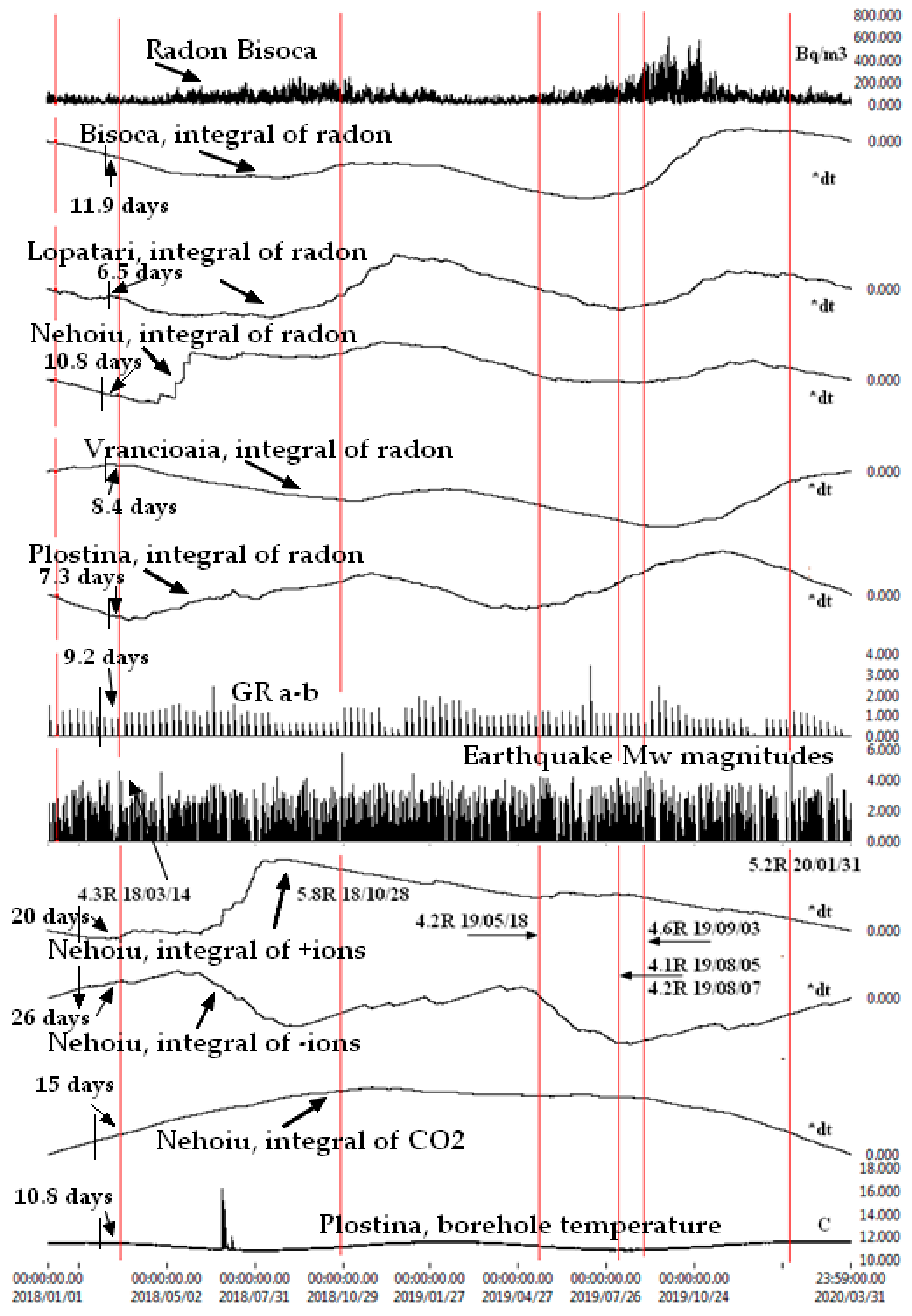
| 18/03/14 | 4.6/ 137 Km | 17.3 | Radon BISRd | slope-,dt | 11.9 | 1 |
| 24.23 | Radon LOPRd | slope-,dt | 6.5 | 1 | ||
| 35.3 | Radon NEHRd | slope-,dt | 10.8 | 1 | ||
| 26.68 | Radon VRId | slope-,dt | 8.4 | 1 | ||
| 31.5 | Radon PLRd2 | slope-,dt | 7.3 | 1 | ||
| GR a-b | slope+,dt | 9.2 | 1 | |||
| 35.3 | +Ions NEHR | slope-, min | 20 | 1 | ||
| 35.3 | -Ions NEHR | slope+, max | 26 | 1 | ||
| 35.3 | NhCO2 | slope-,dt | 15 | 1 | ||
| 31.5 | Tf PLOR | dt | 10.8 | 1 | ||
| 2018/06/14 | GR a-b | 0 | ||||
| 2018/06/27 | Tf PLOR | 0 | ||||
| 2018/07/02 | Radon VRId | 0 | ||||
| 2018/07/08 | Radon NEHRd | 0 | ||||
| 2018/07/08 | Radon NEHRd | 0 | ||||
| 2018/07/17 | NhCO2 | 0 | ||||
| 2018/08/16 | Radon PLRd2 | 0 | ||||
| 2018/09/29 | Radon LOPRd | 0 | ||||
| 2018/10/16 | Radon LOPRd | 0 | ||||
| 18/10/28 | 5.8/ 148 Km | 30.96 | Radon BISRd | slope+,dt | 20.4 | 1 |
| 20.52 | Radon LOPRd | slope+,dt | 9.6 | 1 | ||
| 21.12 | Radon NEHRd | slope+,dt | 9.6 | 1 | ||
| 40.07 | Radon VRId | slope-,dt | 39.6 | 1 | ||
| 37.56 | Radon PLRd2 | slope+,dt | 13.2 | 1 | ||
| GR a-b | slope+,dt | 12 | 1 | |||
| 21.12 | Ions+ Nehoiu | slope- | 33 | 1 | ||
| 21.12 | Ions- Nehoiu | slope+ | 33 | 1 | ||
| 21.12 | NhCO2 | slope-,dt | 21 | 1 | ||
| 40.77 | Tf PLOR | dt | 56 | 1 | ||
| 18/11/18 | Radon LOPRd | 0 | ||||
| 18/11/28 | +Ions NEHR | 0 | ||||
| 18/11/28 | -Ions NEHR | 0 | ||||
| 18/12/07 | Radon LOPRd | 0 | ||||
| 18/12/16 | NhCO2 | 0 | ||||
| 18/12/21 | -Ions NEHR | 0 | ||||
| 19/01/08 | Tf PLOR | 0 | ||||
| 19/01/12 | Radon BISRd | 0 | ||||
| 19/01/30 | +Ions NEHR | 0 | ||||
| 19/01/30 | -Ions NEHR | 0 | ||||
| 19/02/15 | Radon NEHRd | 0 | ||||
| 19/02/18 | Radon LOPRd | 0 | ||||
| 19/04/07 | +Ions Nehoiu | 0 | ||||
| 19/04/07 | -Ions Nehoiu | 0 | ||||
| 19/04/13 | Radon LOPRd | 0 | ||||
| 19/04/22 | Radon VRId | 0 | ||||
| 19/05/21 | GR a-b | 0 | ||||
| 19/07/14 | Radon PLRd2 | 0 | ||||
| 19/09/03 | 4.6/ 119 Km | 37.23 | Radon BISRd | slope+,dt | 21.2 | 1 |
| 24.5 | Radon LOPRd | slope+,dt | 15.6 | 1 | ||
| 7.16 | Radon NEHRd | slope+,dt | 8.4 | 1 | ||
| 57.39 | Radon VRId | slope-,dt | 37.3 | 1 | ||
| 54.41 | Radon PLRd2 | slope+,dt | 9.6 | 1 | ||
| GR a-b | slope+,dt | 10 | 1 | |||
| 7.16 | +Ions NEHR | slope-, max | 16 | 1 | ||
| 7.16 | -Ions NEHR | slope+, min | 16 | 1 | ||
| 7.16 | NhCO2 | slope-,dt | 19.3 | 1 | ||
| 54.41 | Tf PLOR | dt | 94 | 1 | ||
| 19/09/09 | Radon BISRd | 0 | ||||
| 19/10/09 | Radon PLRd2 | 0 | ||||
| 19/10/14 | Radon NEHRd | 0 | ||||
| 19/10/08 | Radon BISRd | 0 | ||||
| 19/10/31 | Radon BISRd | 0 | ||||
| 19/10/18 | Radon LOPRd | 0 | ||||
| 19/10/25 | NhCO2 | 0 | ||||
| 19/10/27 | Tf PLOR | 0 | ||||
| 19/11/05 | Radon VRId | 0 | ||||
| 19/11/05 | GR a-b | 0 | ||||
| 19/11/13 | Radon LOPRd | 0 | ||||
| 19/12/15 | Radon PLRd2 | 0 | ||||
| 19/12/31 | Radon LOPRd | 0 | ||||
| 20/01/31 | 5.4/ 118 Km | 14.19 | Radon BISRd | slope-,dt | 12.5 | 1 |
| 24.87 | Radon LOPRd | slope-,dt | 8.4 | 1 | ||
| 40.53 | Radon NEHRd | slope-,dt | 10.8 | 1 | ||
| 20.18 | Radon VRId | slope+,dt | 37.3 | 1 | ||
| 21.87 | Radon PLRd2 | slope-,dt | 12.4 | 1 | ||
| GR a-b | slope+,dt | 22 | 1 | |||
| 40.53 | +Ions NEHR | slope-, max | 36 | 1 | ||
| 40.53 | -Ions NEHR | slope+, min | 36 | 1 | ||
| 40.53 | NhCO2 | slope-,dt | 55 | 1 | ||
| 21.87 | Tf PLOR | dt | 21 | 1 |
Publisher’s Note: MDPI stays neutral with regard to jurisdictional claims in published maps and institutional affiliations. |
© 2020 by the authors. Licensee MDPI, Basel, Switzerland. This article is an open access article distributed under the terms and conditions of the Creative Commons Attribution (CC BY) license (http://creativecommons.org/licenses/by/4.0/).
Share and Cite
Toader, V.-E.; Nicolae, V.; Moldovan, I.-A.; Ionescu, C.; Marmureanu, A. Monitoring of Gas Emissions in Light of an OEF Application. Atmosphere 2021, 12, 26. https://doi.org/10.3390/atmos12010026
Toader V-E, Nicolae V, Moldovan I-A, Ionescu C, Marmureanu A. Monitoring of Gas Emissions in Light of an OEF Application. Atmosphere. 2021; 12(1):26. https://doi.org/10.3390/atmos12010026
Chicago/Turabian StyleToader, Victorin-Emilian, Víctor Nicolae, Iren-Adelina Moldovan, Constantin Ionescu, and Alexandru Marmureanu. 2021. "Monitoring of Gas Emissions in Light of an OEF Application" Atmosphere 12, no. 1: 26. https://doi.org/10.3390/atmos12010026
APA StyleToader, V.-E., Nicolae, V., Moldovan, I.-A., Ionescu, C., & Marmureanu, A. (2021). Monitoring of Gas Emissions in Light of an OEF Application. Atmosphere, 12(1), 26. https://doi.org/10.3390/atmos12010026