Article

Road Traffic Dynamic Pollutant Emissions Estimation: From Macroscopic Road Information to Microscopic Environmental Impact

by
Giovanni De Nunzio
,
Mohamed Laraki
and
Laurent Thibault
*,†
IFP Energies nouvelles, Rond-Point de l’échangeur de Solaize, BP 3, 69360 Solaize, France
*
Author to whom correspondence should be addressed.
These authors contributed equally to this work.
Atmosphere 2021, 12(1), 53; https://doi.org/10.3390/atmos12010053
Submission received: 30 November 2020 / Revised: 27 December 2020 / Accepted: 27 December 2020 / Published: 31 December 2020
(This article belongs to the Special Issue Air Pollution and Environment in France)

Abstract

:
Air pollution poses a major threat to health and climate, yet cities lack simple tools to quantify the costs and effects of their measures and assess those that are most effective in improving air quality. In this work, a complete modeling framework to estimate road traffic microscopic pollutant emissions from common macroscopic road and traffic information is proposed. A machine learning model to estimate driving behavior as a function of traffic conditions and road infrastructure is coupled with a physics-based microscopic emissions model. The up-scaling of the individual vehicle emissions to the traffic-level contribution is simply performed via a meta-model using both statistical vehicles fleet composition and traffic volume data. Validation results with real-world driving data show that: the driving behavior model is able to maintain an estimation error below 10% for relevant boundary parameter of the speed profiles (i.e., mean, initial, and final speed) on any road segment; the traffic microscopic emissions model is able to reduce the estimation error by more than 50% with respect to reference macroscopic models for major pollutants such as NOx and CO2. Such a high-resolution road traffic emissions model at the scale of every road segment in the network proves to be highly beneficial as a source for air quality models and as a monitoring tool for cities.

1. Introduction

The World Health Organization (WHO) classified outdoor air pollution as a carcinogen at the end of 2013. In Europe, air pollution is the leading environmental health risk. According to the WHO and the Organisation for Economic Co-operation and Development (OECD), outdoor and indoor air pollution caused 663,000 premature deaths in the European region in 2010. The limit values set by the European Commission are repeatedly exceeded on European territory and in particular on French territory. Faced with this observation, the European Commission has initiated legal proceedings against 17 countries, including France, for failure to comply with the standards for PM10 particles (and insufficient reduction actions, particularly for France). This litigation reached a further stage on 19 June 2015, with the European Commission calling on France to take the necessary measures to meet its obligations, the last step before referral to the Court of Justice. Finally, in October 2019, within the Judgment in Case C-636/18 Commission v France, the Court of Justice of the European Union upheld the Commission’s action and found that France had failed to fulfill its obligations under the Air Quality Directive.
On the other hand, the European Environment Agency recently emphasized that cities lack simple and easy-to-use methodologies and tools to quantify the costs and effects of their measures and assess those that are most effective in improving air quality. Transportation is one of the most pollutants emitting sectors [1]. In real driving conditions, vehicles’ pollutant emissions depend not only on the vehicle technology, but also on the driving style, the road infrastructure and the traffic regulation measures. Changes in road infrastructure and traffic management are frequent, especially in urban areas. Capacity, congestion, and safety of users are often the only decision criteria. Impact on pollutant emissions is rarely, if ever, taken into account, and only a few infrastructure owners are in a position to make such optimization decisions [2]. However, changes in road infrastructure and traffic management may have a strong impact on driving conditions and vehicle emissions as shown by some studies [3].
Advances in Intelligent Transportation Systems (ITS) and Traffic Information Systems (TIS) are making it increasingly easy to access traffic data. This opens possibilities for innovative models and methods for traffic related predictions. In particular, estimating driving behavior and dynamic speed profiles with realistic acceleration content and updating such information at regular time intervals to better take into account time-varying traffic conditions is of particular interest.
Most of the speed estimation methods are traditionally based on a single mean value estimation per road link. They use real-world traffic data collected from probe vehicles or various monitoring systems, in particular Loop Detectors (LP) and Floating Car Data (FCD) [4,5,6,7]. The usage and accuracy of these methods, however, depend on the availability of real-world traffic data.
Traffic models can be used to estimate road link speed. They exploit the fundamental diagram theory [8,9] to describe the deterministic relationship between the flow speed and the density (number of vehicles per unit length). Macroscopic models consider the aggregate behavior of traffic flow on road links and estimate a mean speed in a road link. In microscopic models [10,11], each vehicle is considered separately and the interactions are mostly based on car-following and lane-changing theories. All these models, however, require some complex calibration and extensive inputs (Origin/Destination matrix, etc.) that might not be available for any road network.
Driving cycles are also used for the generation of realistic speed trajectories. They are constructed from a history of real trips and use stochastic approaches [12,13]. However, these driving cycles are generally used for large distances and they do not really take into account the impact of the topology and infrastructure at a high resolution. Alternatively, parametric spline functions can be used in the cases of traffic lights, stop signs and roundabouts [14]. Polynomial functions are proposed in [15] to construct speed profiles of turning vehicles at signalized intersections.
Models for acceleration have been considered, particularly in [16] (based on heuristic assumptions) or [17]. Such models often fail to predict stopping points, related for instance to traffic lights or intersections. To do so, speed trajectory classification might be used, as in [18], where clustering algorithms are used to identify three major patterns at a specific intersection.
In this work, we build on the results of [19] and extend the application of the driving behavior model to the road traffic emissions’ estimation with extensive validation and comparison results. In fact, this information can be used for a better overall understanding of the phenomena and the factors generating traffic-related pollutant emissions at high spatial and temporal resolution. Solutions can then be found to improve traffic safety and reduce overall emissions and energy consumption.
In order to accurately estimate pollutant emissions from the predicted driving behavior, an adapted microscopic vehicle and emissions model should be used. Indeed, the pollutant emissions level is strongly linked to the driving behavior, regardless of the vehicle and its technologies. This sensitivity is much higher than for fuel consumption. For a same itinerary, and with the same car, the level of pollutant emissions can be tripled between two drivers, depending on how they drive. A better knowledge and monitoring of vehicle usage will have a double benefit: at the driver scale, a direct decrease of emissions through improved driving behavior and habits; at the regulator scale, assisting the development of future standards and infrastructures.
Regarding the microscopic emissions modeling, for a long time, the environmental impact of vehicles has only been evaluated by the means of dynamo-meter emissions tests. The data derived from such testing is not representative of “real-world” driving conditions [20]. To deal with this issue, the Portable Emissions Measurement System (PEMS) has been being developed since the 1990s [21]. These systems are suitable for measurements on a specific vehicle; however, due to their cost, large scale studies of real driving emissions (RDE) are not possible. As a consequence, little is known about the impact of real-world conditions on emissions and only very recently studies have been starting to shed more light on the subject [22,23]. A way to measure indirectly real traffic emissions of vehicles is to use an air quality sensor, but large scale diffusion is limited as well, and it is then difficult to relate the pollution to its cause. It is known that emission factors can be coupled with real GPS data to estimate vehicle emissions [24]. However, emission factors only consider average vehicles and average driving style and are suitable for average emissions on long trips but not for real traffic emissions which needs to take into account the local impact of the driving style and slope [25]. To take into account these phenomena, it is necessary to use a finer level of model called microscopic, whose input is generally a 1 Hz vehicle speed profile. Several microscopic models already exist, but they are designed for offline studies [26]. They are often coupled with microscopic traffic simulators which provide the 1 Hz speed profile [27,28]. Unfortunately, there is an important gap between simulated and measured speed profiles and therefore pollutant emissions, as illustrated in [29]. The purpose of this work is to couple a new microscopic emissions model, covering even the most recent pollutants after-treatment technologies, unlike other renowned microscopic emission models, such as PHEM [30], with realistic speed profiles provided by the proposed driving behavior model to estimate on-road pollutant emissions.
The objective of this work is to propose a modeling framework to estimate vehicular traffic pollutant emissions in each segment of a road network by only using macroscopic topographic and traffic information. Firstly, the proposed approach focuses on designing a generalized approach for the estimation of vehicle speed trajectory at a road link scale. This driving behavior model is trained on the real-world speed trajectories recorded by the smartphone application Geco air [31]. This application records automatically the 1-Hz Global Positioning System (GPS) signal when the user is moving to provide him a feedback on the individual environmental footprint of his mobility. The application is free to download and use. In addition to encouraging the users to take part in a citizen science project, the application provides drivers with an individual coaching to reduce their pollutant and CO2 emissions. The resulting database is usable for research purposes and compliant with General Data Protection Regulation (GPDR) rules. It is a major opportunity to improve the understanding of real-word driving conditions and related emissions which are now modeled in a really simplified way to predict the pollutant concentrations. In 2020, this database counts more than 6 Million trips for a total of 73 Million kilometers, and these figures increase continuously with the daily trips of thousands of users. The driving behavior model trained with these data are then used to estimate speed trajectories on any road link, not requiring the availability of previous recordings on the considered road links. The model does not need any calibration and takes as inputs macroscopic data (road infrastructure, topology, etc.) that are available through commercial Geographic Information System (GIS). A stochastic approach is exploited to construct vehicle speed trajectories. This allows the estimation of several speed trajectories per road link, to take into account various possible driving behaviors. Secondly, a microscopic vehicle and pollutant emissions model is proposed to be able to convert the estimated driving behavior into vehicle emissions at the outlet of the exhaust-line. Lastly, the vehicle emissions are converted into the emissions of an equivalent vehicle representing the vehicles fleet circulating in the considered area obtained from public statistical studies. The calculation of the overall road traffic emissions on every link of the road network is then performed by considering the traffic volume estimated in the network by traffic detectors or traffic models.
The contributions of this work are twofold:
  • The proposed modeling framework is able to estimate time-varying and microscopic road traffic emissions by only using easily obtainable macroscopic topographic and traffic information on any given geographical area;
  • A thorough model validation is able to highlight the model accuracy and the drastic emissions estimation error when compared to well-established macroscopic emissions models, such as COPERT [32]. In addition, our model is able to identify critical road links in terms of pollutant emissions at a very high spatial resolution. Such a precision is very valuable to understand what road segments should need careful investigation and perhaps infrastructure modification, as well as to feed atmospheric dispersion and air quality models with high-resolution emission sources.
The paper is organized as follows: Section 2 describes the modeling framework comprising the driving behavior model, the employed microscopic emissions model, and the meta-modeling approach to convert individual vehicle emissions into road traffic emissions. Finally, a thorough validation analysis of each constituting block of the proposed model is given in Section 3. Concluding remarks and main results are summarized in Section 4.

2. Materials and Methods

As previously mentioned, the objective of this work is to estimate vehicular traffic pollutant emissions in each segment of a road network by only using macroscopic topographic and traffic information. In the following, the methodology and the main modeling blocks proposed to attain this goal are described in detail. An illustration of the modeling framework is shown in Figure 1.

2.1. Driving Behavior Model

Real-world driving speed measurements are not available everywhere and generally difficult to obtain. Nowadays, the advent of vehicles connectivity and intelligent transportation systems is making driving data increasingly easy to acquire. However, often, the spatial and temporal coverage of these data are not sufficient to establish an accurate driving behavior model on each segment (or link) of the road network. Thus, in order to predict driving behavior on any road link, even in the absence of pre-recorded driving data, the proposed model aims to relate macroscopic road and traffic data available everywhere through commercial GIS (e.g., HERE Maps [33]) to typical dynamic (i.e., time-variant) vehicle speed trajectories. The proposed driving behavior model is defined in a machine learning framework as a sequence of cascaded sub-models which are inspired by empirical observation of real-world driving and traffic data. For the design and training of the model, we used a data-set of real-world driving Floating Car Data recorded with the Geco air application in the Greater Paris and Lyon area (France), consisting of approximately 200 thousand road segments and over 2 million data samples, or observations (i.e., driving profiles). The structure of the model is illustrated in Figure 2 and discussed in detail in the following.

2.1.1. Road Network Segmentation

When looking at the speed trajectories recorded on a given road link, it is often observed that a large variety of trajectories exist and the associated statistical dispersion is high. This is due to several factors impacting driving behavior on a same road link: congestion levels, driving style, state of signalization, driving intentions with upstream and downstream maneuvers, etc. In order to reduce statistical dispersion, the first step of the model aims to separate driving maneuvers by redefining the road network as a list of link triplets. Each road link generates a set of road link triplets, covering all the origin and destination options for the considered road link. Each of these triplets is then composed by the considered road link in the middle, plus an origin road link upstream and a destination road link downstream. The road network redefinition in the triplets framework is then performed in two steps: (i) divide the considered network into its constituting unit road links; (ii) from the unit road links, build all the generated triplets.

2.1.2. Driving Behavior Categorization

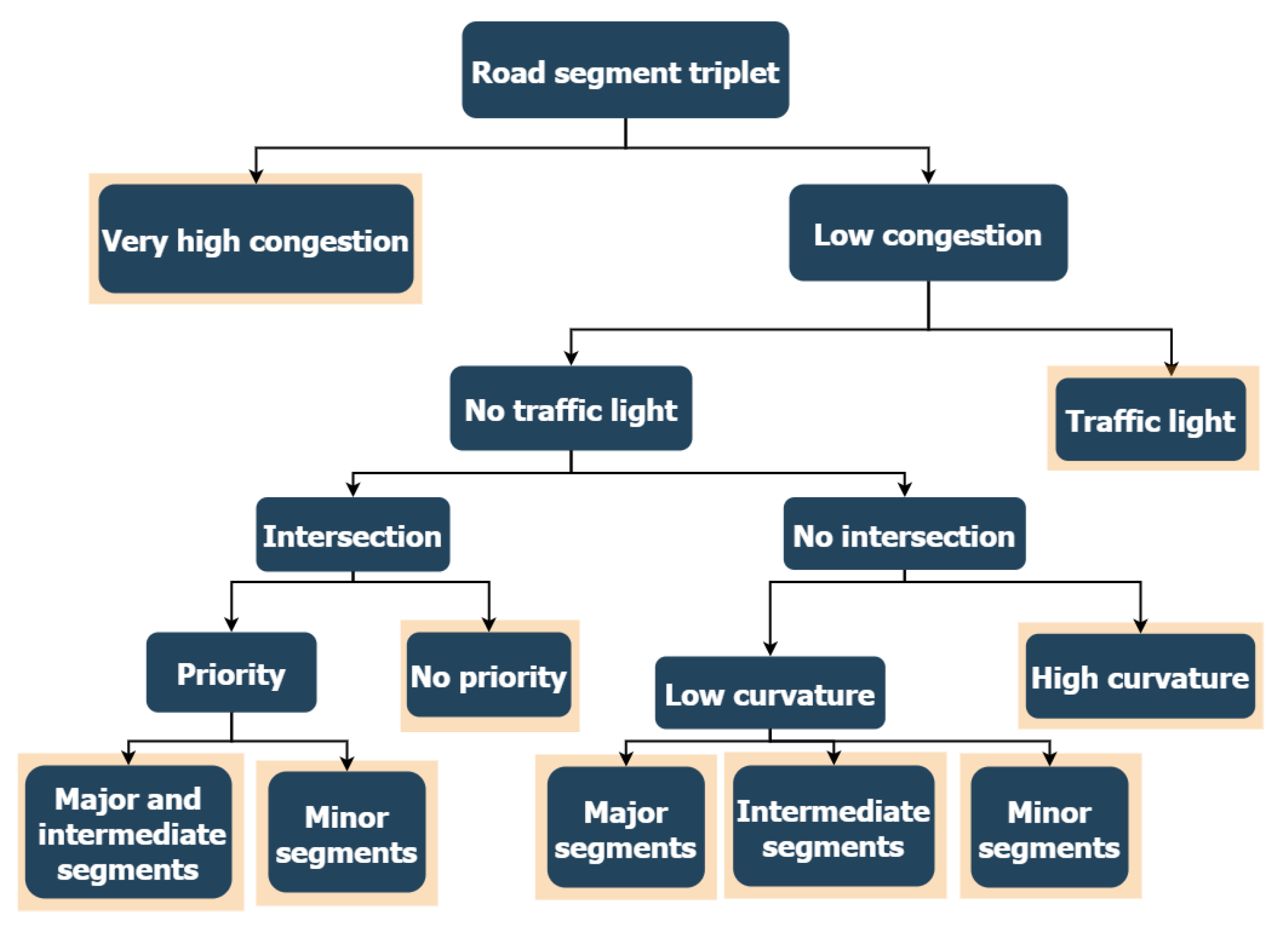
Speed trajectories on the center road links of triplets share the same driving intentions in terms of maneuvers, and thus they have similar shapes and characteristics and a lower statistical dispersion, as observed in real-world driving data. In this second step of the driving behavior modeling approach, a heuristic decision tree is built only from macroscopic road features and traffic conditions (signalization, road curvature, connectivity, traffic congestion, etc.). The decision tree is used to group similar speed characteristics in a same category (a tree leaf in Figure 3). Each category is defined based on chosen macroscopic features that are reported in Table 1.
  • Very high congestion: The congestion level, which is the ratio between the traffic speed and the free-flow speed, is below a defined threshold.
  • Traffic light: Traffic light presence in the middle road link of the triplet.
  • No priority: Existence of stop or yield sign in the middle road link of the triplet. It is also the case if the destination road link has lower functional importance than the other downstream road links.
  • Priority—Major and intermediate segments: The destination road link has more functional importance than the other downstream road links. The triplet is a motorway, a major road link, or a secondary road link with high volume traffic.
  • Priority—Minor segments: The destination road link has more functional importance than the other downstream road links. The triplet is a minor road link with low volume traffic and low-speed limitation.
  • High curvature: The triplet curvature is above a defined threshold.
  • Low curvature: The triplet curvature is below a defined threshold. Then, three categories are defined based on their functional importance within the Transportation Network.
Those categories are based on heuristic assumptions. For instance, in the high congestion case, where the traffic speed is significantly lower than the free-flow speed, the vehicle’s speed is very low and neither the signalization nor the curvature have a significant impact on the driving behavior. In other words, based on observations, when the average speed is low, it is difficult to distinguish between infrastructure-induced stops and traffic-induced stops. The same reasoning is applied for the traffic light case: speed trajectories tend to show the same behaviors in a traffic light case whether there is an intersection or not. Following this heuristic process, nine easily interpreted categories are defined. With the recorded speed database used for training, the categories have a balanced data distribution. Apart from the high curvature case, each category contains between 10 and 20% of the training database. The high curvature case only represents 3% of the training database, as such high curvatures are not common in the urban areas of Paris and Lyon.

2.1.3. Clustering of Driving Styles

For each category, we then consider all the recorded speed trajectories on the center road links of all triplets belonging to the category. On this collection of speed trajectories, we apply a clustering algorithm in order to determine a set of driving speed clusters for each category. The objective of such a clustering phase is to identify the most representative driving behaviors and to further reduce statistical dispersion of the real-world speed profiles belonging to a certain link triplet, which in turn belongs to a certain category of the decision tree. In other words, while the triplets aim to group driving behaviors associated with the same maneuver, and categories group driving behaviors associated with same macroscopic road features, the clusters aim to group driving behaviors associated with similar dynamic content (e.g., stop at a red traffic light, aggressive driving, etc.).
A clustering method, based on the microscopic features reported in Table 2, is used to identify similar driving behaviors. Those features are computed for every recorded speed trajectory in a triplet, and have been chosen to identify the most representative speed dynamics characteristics.
The squared Euclidean distance is used for clustering, distances being computed from normalized values of the microscopic features. Note that it is not mandatory to use all the proposed features for all the categories. For each feature x, a minimum value x min (resp. a maximum value x max ) is computed, as the 5th percentile (resp. 95th percentile) of the distribution of x. This helps to remove outliers. The normalized value is then computed as ( x x min ) / ( x max x min ) .
Since all the features are numerical and the database is very large, the K-means clustering algorithm was used for its efficiency and convergence speed [34]. The silhouette metric [35] was used to evaluate the optimal number of clusters. The silhouette of a point i in the space of normalized microscopic features is defined as S i = ( b i a i ) / max ( a i , b i ) , with a i being the average distance to the other points in the cluster and b i the minimum average distance from the points in the other clusters. By definition, S i [ 1 , 1 ] .
For a category, the number of clusters was varied from 1 to 10 and the optimal number of clusters was identified as the one maximizing the silhouette metric. A key advantage of using this metric is its consideration of how close a point is to a cluster while comparing it to the minimal average distance to another cluster. A negative mean silhouette value means that the point is closer to another cluster. A mean silhouette value higher than 0.5 indicates a generally good clustering, in which each point is well matched to its own cluster, and poorly matched to other clusters.
The mean value of the mean silhouette metrics for all the categories is about 0.53, with the minimum value being equal to 0.43 for the “Intermediate segments” category. In total, 29 clusters are identified for the nine categories. Apart from providing good clustering results, combining the silhouette metric with the K-means algorithm allows for the identification of speed clusters that can be physically interpreted. For each cluster, the dispersion level is very low and a typical driving behavior can be identified.
Finally, the proportion of recorded speed trajectories that each cluster groups can be used to estimate occurrence probabilities of each cluster. Such probabilities are an important property of the proposed driving behavior model and of the speed trajectories’ construction from macroscopic variables.

2.1.4. Driving Characteristics Extraction

In the model, the clusters obtained in the previous step serve two purposes. First, macroscopic variables can be linked to the clusters’ features: initial speed v i (at the inlet of the center road links), final speed v f (at the outlet of the center road links), plus a possible stop S within the center road links. Such a stop is defined by the relative positions of the stops from the outlets of the center road links.
Once the relationship has been established, any triplet is linked, through macroscopic variables only, to a set of vectors D = ( v i , v f , S ) for each cluster.
A random forest (RF) regression algorithm [36] is used to estimate the initial speed v i and final speed v f for each cluster. The stopping point position S is also estimated for some clusters. This supervised learning algorithm takes as inputs the previously defined clusters and remaining macroscopic features, not used for the decision tree. Apart from the traffic speed, these macroscopic features are computed for the center road links associated with the cluster. For a cluster C,
[ v i , v f , S ] = RF ( C , N l , V O t , V t , V D t , V n , L s , α s , α c , N i , N f )
The definition of the RF inputs is given in Table 3. Bagging is used as the random forest training method. It is an ensemble learning method which involves random sampling of small subsets of data from the dataset. The selection of all the examples in the dataset has equal probability. Each tree of the random forest learns from a different subset. By doing so, the random forest model has a higher stability with less possible over-fitting.
The proposed learning scheme also includes iterations on its inputs and structure using K-fold cross validation [37]. This allows for better tuning the model and obtaining the optimal topology while avoiding over-fitting. The basic idea is to test different hyper-parameters and choose the ones with the best associated performance in the training, test, and validation datasets. The supervised learning algorithm performance is assessed in terms of the coefficient of determination R2:
R 2 = 1 j = 0 n ( y j y j ^ ) 2 / j = 0 n ( y j y ¯ ) 2
where n is the number of measurements, y j is the j t h measurement value, y j ^ is the related estimated value, and y ¯ is the mean measurement value. A coefficient of determination close to 1 means that the estimations and measurements are perfectly correlated. As a result of the K-fold cross validation, the coefficient of determination is higher than 0.9 for the test and validation sets for v i and v f . The stop S also gets good estimation results, with a coefficient of determination equal to 0.81 for the validation set. It is challenging to increase S estimation accuracy, since it depends on other macroscopic variables that are not usually available, like the traffic light exact position for instance. In addition, in a very congested case, the S position can be anywhere on the road link.
As with any supervised learning algorithm, the prediction accuracy depends on the data quality. The data should be exhaustive for each model input dimension. In our case, 22% of the data are redundant. This means that a similar prediction accuracy is obtained with the remaining 78% of the data. In this case, the proposed supervised learning algorithm convergence time is approximately 1 h on a laptop computer equipped with a Central Processing Unit (CPU) at 2.8 GHz and 16 GB of Random Access Memory (RAM).
Apart from the satisfying estimation results, the random forest bagging trees algorithm estimates the mean and also the standard deviation of each variable to be estimated. Accordingly, speed trajectories parameters ( v i , v f and S) can be generated with a Gaussian distribution to take into account the stochastic nature of the driving behavior. This is exploited in the construction of speed profiles presented in the next step of the model.

2.1.5. Stochastic Speed Construction

The last step of the model consists of computing speed trajectories for each vector D of each cluster. Let us recall that a cluster groups a part of all the speed trajectories of the center road links of triplets that belong to the same category. This means that the recorded speed profiles belonging to a cluster, although sharing similar characteristics, may have very different duration due to the different lengths of the road links. Therefore, we first normalize the description of these speed trajectories by considering a common variable that is the relative position p from the end of the center road link (from 0 at its inlet, to 1 at its outlet). At each discretization step p k of p, we assign a probability for a k (acceleration at p k ), conditioned to a k 1 (previous acceleration), v k 1 (previous speed) and δ k (difference v k 1 v f ). Then, starting from an inlet speed v i , we sequentially construct a speed trajectory. We will see in the sequel that, in practice, a set of less than 10 stochastically constructed speed trajectories suffices to correctly represent driving behavior for a cluster.
For the construction of the vehicle speed trajectory, a probabilistic approach is used: a multi-dimensional discrete Probability Density Function (PDF) approximates the stochastic part of the driving behavior, which deterministic approaches fail to capture.
A PDF is constructed for each cluster, with the associated recorded speed trajectories. It is used to get the next acceleration, based on the following equation:
a k + 1 P ( a k + 1 | a k , v k , δ k , p k )
The parameters used in Equation (3) are computed for each recorded speed trajectory time step in the center road link of a triplet. Then, they are grouped to construct the PDF.
Given v i (obtained with a random draw from its Gaussian distribution, given by the RF algorithm), the next acceleration value is selected according to the constructed multi-dimensional PDF (Equation (3)). Then, the next speed value is computed by adding the computed acceleration to the previous speed. This procedure is repeated until the road link end is reached. For clusters having a stop point, the same process is applied two times: between the initial point and the stop point for the first part, and between the stop point and final point for the second part.
At this point, several dynamic speed trajectories can be constructed on any road link, and only macroscopic road features are needed as inputs.

2.2. Microscopic Emissions Model

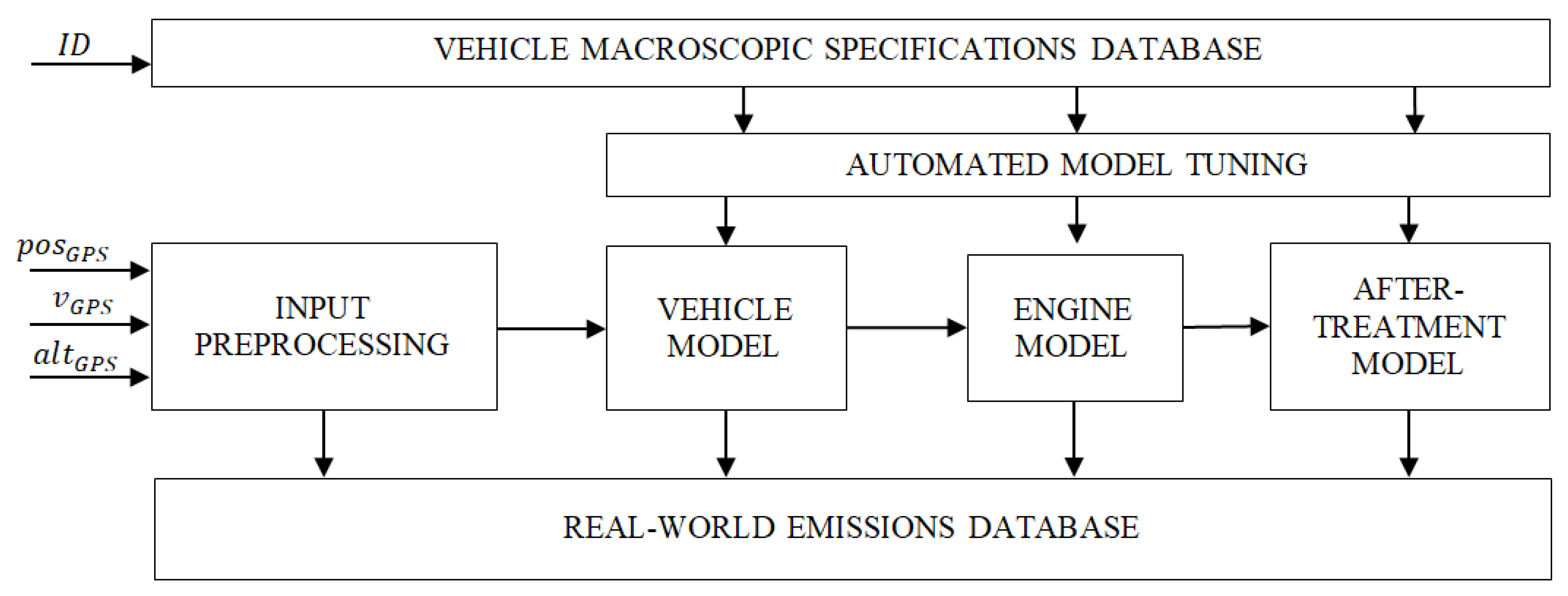
The obtained dynamic speed profiles obtained as an output of the driving behavior model can be now fed into a microscopic energy consumption and emissions model of the vehicle. Figure 4 shows the cloud computing architecture used to estimate pollutant emissions from GPS measurements. The four inputs of this calculation, provided by the user smartphone, are the registration number of the vehicle (ID) and GPS measurements automatically recorded (i.e., position, speed and altitude). For brevity of presentation, this section focuses on emissions of NOx, PM, and CO2 for Diesel vehicles, but the model is applicable to all types of regulated pollutants and vehicle powertrains.
The choice of the right modeling level is a trade-off between precision, number of input parameters, and computation time. The desired models should be able to catch the impact of real-world driving conditions and to identify situations where pollutant emissions are particularly high or low. Moreover, the model has to deal with inputs sampled at low rates, typically 1 Hz, as provided by the GPS sensor of most smartphones. This is a critical point because the creation of pollutant emissions occurs during an engine cycle, typically few milliseconds. An important remark is that the models are not based on the results of a standard driving cycle (such as the New European Driving Cycle (NEDC)), which often fails to represent real on-road conditions. On-road and on-cycle emissions can be widely different for some pollutants and some engine technologies. The models integrate realistic engine and after-treatment calibrations, which is essential for real-world emissions modeling. In the following, we give an overview of the different sub-models composing the overall microscopic emissions model.

2.2.1. Vehicle Model

This model takes into account the vehicle dynamics. It takes two inputs, the GPS speed and altitude, to compute the engine speed and torque. It is based on the longitudinal dynamics of the vehicle, which can be written as:
m d v ( t ) d t = F e n g F r e s F s l o p e F b r k
where F e n g is the traction force of the engine, F b r k is the braking force, F r e s is the friction force due to aerodynamic and rolling resistance, and F s l o p e is the gravitational force. The force at the wheels is then written as:
F w h e e l = F e n g F b r k
These equations allow for computing the engine traction force and then the engine power P e n g :
P e n g = v F e n g ρ t r a n s = ( m d v d t + F r e s + F s l o p e + F b r k ) v ρ t r a n s
where ρ t r a n s is the transmission efficiency. At every time step, the model calculates the reduction ratio between the wheel and the engine crankshaft R e w depending on v and P e n g : R e w = f v , P e n g . It converts then the speed and power from the wheel to the engine torque T e n g and speed N e n g at the crankshaft:
N e n g = v R e w , T e n g = P e n g 30 N e n g π
In the case of a hybrid vehicle, the engine power is not directly proportional to the power necessary to move the vehicle. The power split between the engine and the electric motor is chosen by the energy management strategy. This strategy is modeled to take into account the effects of hybridization functionalities, namely pure electric drive, regenerative braking, and engine operations’ optimizations. This strategy is coupled with a simple model of the electrical components that take into account the impact of battery state of charge variation, especially relevant for plug-in hybrids.

2.2.2. Engine Fuel Consumption Model

The first step of this sub-model is to evaluate the internal physical quantities on the current operating point such as flows, temperatures, and concentrations. These quantities will then be used to estimate the pollutant emissions, as well as the fuel consumption. The model quantities are estimated, based on the following basic assumptions:
  • Maximum torque curve and air-path architecture are known for the engine;
  • Generic law for the friction mean effective pressure (FMEP), as a function of engine speed;
  • Constant gross indicated efficiency;
  • Fuel air equivalence ratio equal to 1 in spark-ignition engines (except at high load where it increases linearly with load), and varying between two values for compression–ignition engines;
  • The exhaust gas recirculation (EGR) fraction is known for each point of the engine map.
  • The engine coolant temperature is modeled using a simple heat exchange model. This model takes into account the heat produced by the combustion which is assumed to be a function of the engine operating point and the ambient heat exchange. Cold start effect on fuel consumption is then modeled with a coefficient function of the coolant temperature.
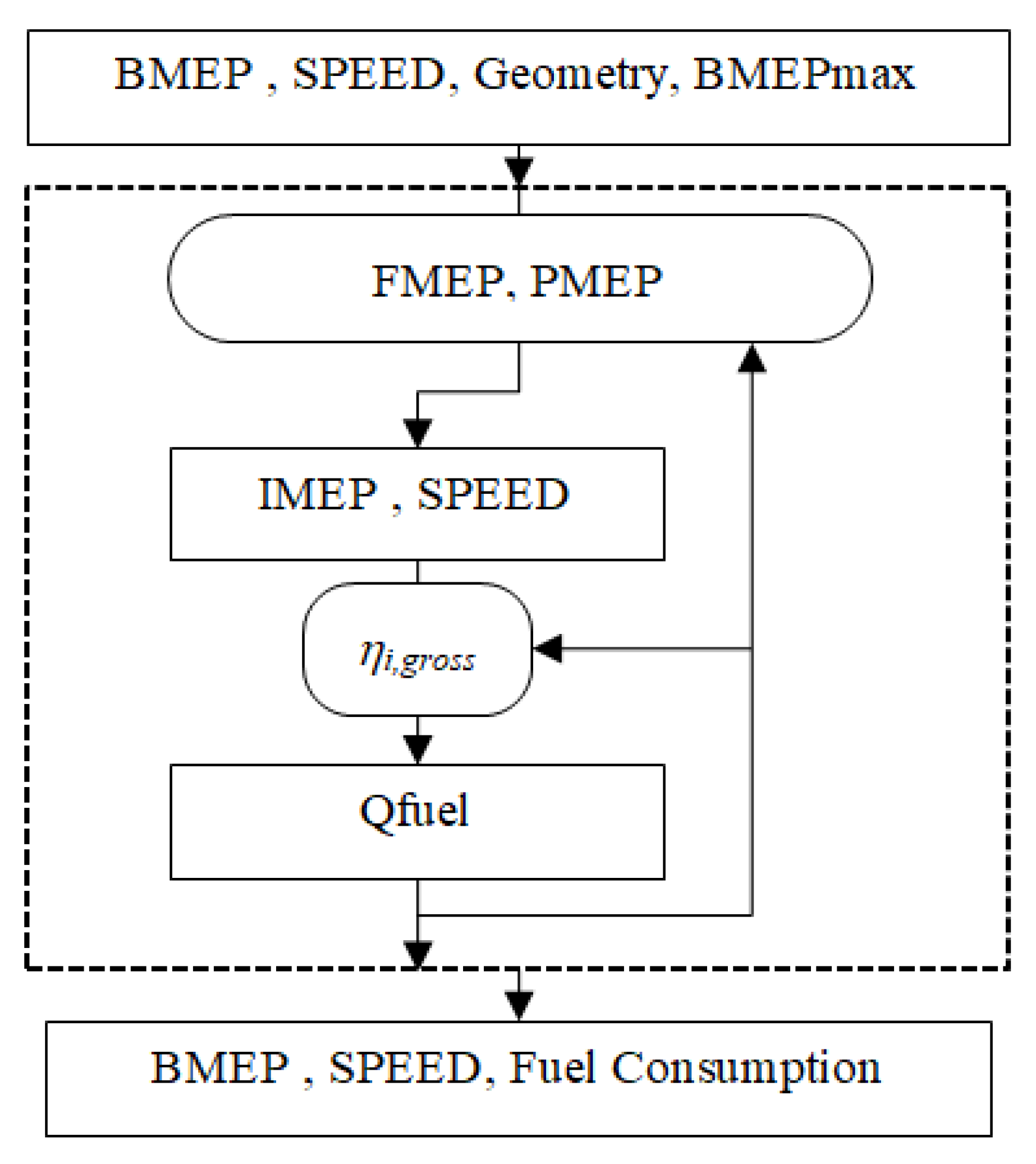
These assumptions are combined in the iterative algorithm presented in Figure 5, and applied for each point of the engine map to determine the pumping mean effective pressure (PMEP), to deduce gross indicated mean effective pressure (IMEP) and fuel consumption, considering the gross indicated efficiency assumption.
Thus, the iterative process is mainly aimed at computing engine fuel consumption and PMEP, which require computing for each point of the engine map the air mass flow rate (with equivalence ratio assumption) and the exhaust temperatures necessary for the pollutant models, as well as the different pressures and temperatures in the air path. The equations used to determine fuel consumption, total intake mass flow rate, and pressure and temperature conditions in the air path are detailed in [38] for engines without EGR.
These equations have been adapted for engines with EGR to improve the exhaust mass flow rate estimation given to the emissions model. Basically, this adaptation ensures that: Q e x h = Q e x h , t o t 1 E G R with Q e x h the exhaust mass flow rate, Q e x h , t o t the total exhaust mass flow rate coming from the cylinders, and E G R the fraction of exhaust gas recirculated given for the engine operating point. Fuel consumption maps generated with this model are consistent with measurements and overall they show estimation errors below 10% compared to test-bench measurements.

2.2.3. Engine-Out Emissions Model

The estimation of engine-out emissions is made using a physical modeling of the engine using mostly equations of the literature with some adjustments to the available data. This modeling is based on steady-state assumptions (i.e., assuming stationary operations) for most parameters, but transient phenomena, such as the air path settling time and thermal behaviors, are included using dynamic models. The cold-start effect is therefore captured with a model that estimates the engine temperature at each time step. One of the main contributions of this work is the NOx emissions models for Diesel engines which is inspired from a semi-empirical model presented in [39]. The original model was:
log ( N O x ) = a 0 + a 1 C O C + a 2 m c y l + a 3 m O 2
with N O x the mass of NOx per mass of fuel, the center of combustion (COC) (50% energy conversion, from Top Dead Center (TDC)) and m c y l and m O 2 the in-cylinder air and oxygen mass per stroke and displaced volume, and a 0 , a 1 , a 2 , a 3 model coefficients. This model was modified to avoid needing the COC which is quite hard to estimate without engine sensors and to include the strong effect of Exhaust Gas Recirculation (EGR). The new model is:
log ( N O x Q S ) = a 0 + a 1 R B G R
where R B G R is the in-cylinder Burned Gas ratio (BGR) estimated with the air path model taking into account engine calibration and the dynamics of the EGR loop. Once engine-out emissions are estimated, it is necessary to model the after-treatment impact on such emissions.

2.2.4. After-Treatment Model

The developed after-treatment model library is composed of six submodels, each of which represents a physical after-treatment element of the exhaust line: Diesel Oxidation Catalyst (DOC), Diesel Particle Filter (DPF), Selective Catalytic Reduction (SCR), Lean NOx Trap (LNT), Three-Way Catalyst (TWC) and PIPE (referring to a thermal model of a simple pipe between two elements). These elements can be arranged to describe the diversity of exhaust line architectures. As an illustration of this diversity, the most common Diesel exhaust architectures are briefly mentioned thereafter. Most of the pre-Euro5 vehicles only use DOC as an after-treatment device. Euro5 architectures commonly use a close-couple DOC-DPF system. Euro6 standard is commonly addressed by the use of an SCR or an LNT, additionally to the DOC and the DPF. Various architectures exist such as DOC-DPF-PIPE-SCR, DOC-PIPE-SCR-DPF, etc. In particular, all the Euro6 after-treatment architectures can be modeled using combinations of these “standard” submodels. An example of such an arrangement is depicted in Figure 6.
All the submodels take the physical quantities of gas flow rate, temperature, gas composition (sHC, sCO, sNO, sNO2, soot, and sO2) at the element inlet as an input and compute the same quantities at the element outlet as an output. Each variable represents the cross-section-averaged quantity at a given axial location. It is then possible to describe precisely the evolution of the gas temperature and composition through the different elements, and to estimate the tail-pipe pollutant emissions.
Going into further detail, each element is in fact discretized spatially into several “slices” to account for the non-uniform axial distribution of the properties inside the element itself. This approach is fully consistent with classical models of packed-bed catalysts developed since the 1970s (see, e.g., [40]). In particular, several benefits of this approach make it necessary for our application: it leads to realistic dynamics of pollutants conversion efficiencies during heat-up phases (such as start-up and sudden accelerations) and during transient cool down phases as well (pedal release, slow driving), which would not be captured by a simple map-based model. In addition, the models are adapted w.r.t. gas flow rate, allowing us to capture precious information, like a drop in conversion efficiency as the engine load is increased.
Other noteworthy model features include capturing catalyst light-off phenomenon, taking into account SCR and LNT control laws to compute conversion, handling of the engine shut-off for conventional vehicles and Hybrid Electric Vehicles (HEVs). Real time-to-execution time ratios as high as 8000 have been measured on a classical laptop to simulate a full DOC-DPF-PIPE-SCR Diesel exhaust line on transient cycles, which perfectly meets our needs in terms of computational burden.

2.3. Microscopic Traffic Emissions

The third and last block of the proposed modeling approach aims to combine the driving behavior model and the single-vehicle microscopic emissions model and to extend the results at the traffic level. In other words, once the pollutant emissions of one vehicle are calculated on one road link based on the estimated driving behavior, it is necessary to calculate the overall emissions of all the vehicles in the whole road network under analysis.
In order to compute the contribution to the overall emissions of all possible vehicle powertrains and after-treatment technologies, the vehicle fleet composition in the considered geographic area needs to be estimated. In this work, the estimation of the vehicle fleet composition is not addressed, and it is considered as a data source. For brevity of presentation, let us consider that the statistical vehicle fleet composition is given and retrieved from available public reports [1]. More precisely, the vehicle fleet composition gives accurate estimates of the proportion of light-duty, commercial and heavy-duty vehicles on every road link of the considered area. Note that all vehicle powertrains and after-treatment technologies from Euro 1 to Euro 6 emission standards are defined in the microscopic emissions model described in the previous section. The equivalent emissions of a vehicle representing the entire fleet are simply obtained via a weighted sum of the individual emissions of each vehicle type indicated in the fleet composition, where each weight corresponds to the proportion of each vehicle in the total fleet composition.
Furthermore, in order to correctly evaluate the impact of traffic volume on the pollutant emissions, the emissions of the equivalent vehicle representing the whole fleet need to be multiplied by the estimated number of vehicles on every road link of the considered road network. Usually, this information is given by macroscopic traffic models calibrated on real-world traffic counts as an average annual daily traffic (AADT). This is also the typical data source and input for other state-of-the-art macroscopic traffic emission models, such as COPERT [32], in which the total traffic emission is obtained as the product of AADT and emission factors as a function of an average driving speed. Note that our approach is microscopic because both the driving behavior model and the vehicle emissions model are dynamic and microscopic (i.e., consideration of speed dynamics, road slope, road infrastructure, traffic levels, temperature dynamics of engine and exhaust-line, etc.). Finally, the microscopic traffic emissions are obtained in this work by multiplying the microscopic emissions of the fleet-equivalent vehicle by the macroscopic traffic volume information AADT.

3. Results

In this work, the experimental results are aimed at validating the proposed modeling approach and at showing the importance of considering microscopic traffic emissions when analyzing the impact of transport emissions on the environment. The results are separated in three main parts.
Firstly, the driving behavior model accuracy was statistically evaluated with respect to real-world recorded speed profiles in the test area. As a reminder, the data-set of real-world driving Floating Car Data was recorded via the Geco air application. For each trip, the available data are the 1 Hz GPS signals (i.e., latitude, longitude, speed, altitude, precision, heading) and the vehicle characteristics (i.e., mass, fuel type, aspiration type, injection type, displacement, Euro norm, after-treatment type).
Secondly, the vehicle microscopic emissions’ model precision was assessed with respect to test-bench measurements, and the model sensitivity to driving style, type of itinerary, and type of vehicle was analyzed in real-world driving conditions via experimental measurements.
Finally, the accuracy of the proposed microscopic traffic emissions model was assessed at the scale of a city neighborhood and in comparison to an established macroscopic emissions model. It should be noted that nowadays the reference methods to estimate traffic emissions on a road network consist of using macroscopic emissions models or emission factors, such as COPERT, and not microscopic models because in general high-frequency real-world driving speed trajectories are not available. Our strategy fills this gap by transforming the macroscopic information available on a geographic area into microscopic traffic emissions thanks to the proposed driving behavior model and the adapted microscopic emissions model. Thus, the proposed strategy does not require any costly microscopic traffic simulation in the test area to generate the driving behavior data, and it can be directly deployed in a new test area, just like the models based on emission factors.

3.1. Driving Behavior Model Validation

The driving behavior model was validated and tested outside of the training data-set. In particular, while the model was trained on real-world driving data recorded in the urban and suburban areas of Paris and Lyon, it was tested in the city of Marseilles. The objective of this validation is to assess the extrapolation capabilities of the model for the dynamic speed profiles construction to be representative even in a different geographical context. The performance of the model was assessed from both a qualitative and quantitative point of view, by evaluating the driving behavior estimation accuracy and the statistical errors with respect to real-world speed profiles recorded in the test area.
In the first part of the validation analysis, the proposed stochastic speed construction method has been compared to a deterministic one. The deterministic approach is based on constructing speed trajectories between v i and v f with first order polynomial functions, the coefficients of which are estimated with the v i and v f values. In a stop case, two first order polynomial functions are used, one between v i and a null speed at S, and the other between the null speed at S and v f .
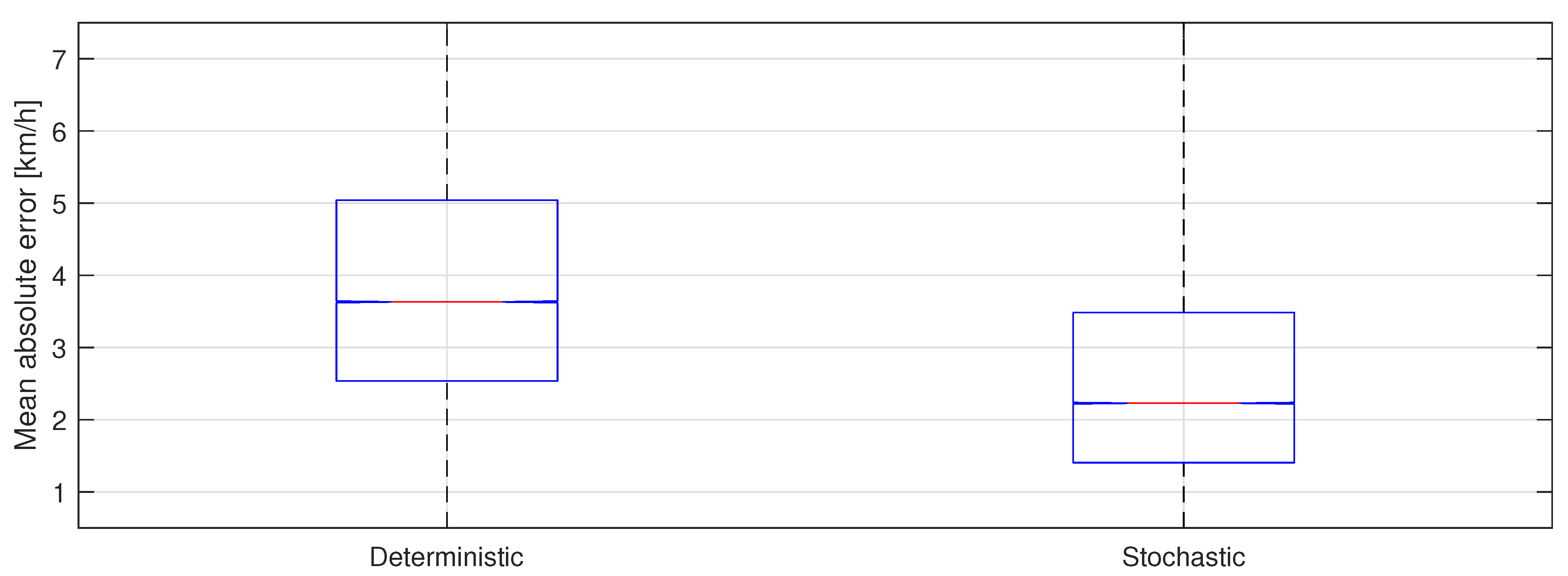
For this comparison, the recorded speed trajectories v i , v f and the S parameters are used for the vehicle speed construction. This allows the evaluation of the stochastic and deterministic approaches errors independently from the random forest estimation accuracy. The mean absolute error distribution between the recorded and the constructed speed trajectories in stop cases is presented in Figure 7. The error median is respectively equal to 3.6 km/h and to 2.1 km/h for the deterministic and the stochastic approaches, with an error reduction of around 40% brought by the stochastic approach. The 75th percentile is reduced by 35% with the stochastic approach with an error distribution more concentrated around the median. The error standard deviation is also reduced by 20% with the stochastic approach. The PDF-based construction is more accurate than the deterministic one. It takes complex driving behaviors into account better, especially in the case of a stop over the road link, or for long road links.
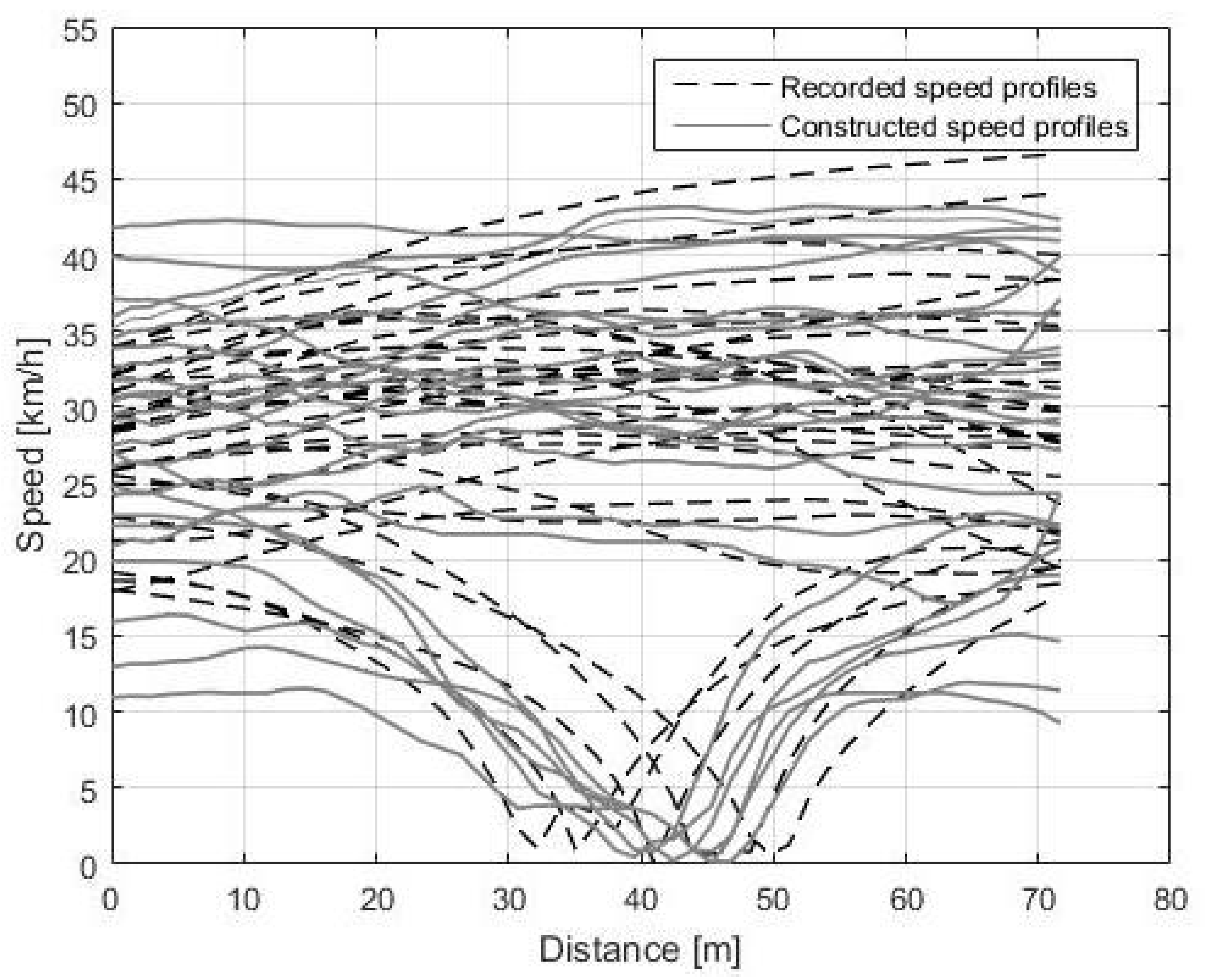
The second part of the validation analysis aims to assess the vehicle speed trajectory parameters estimation accuracy: v i , v f and mean speed v m . Figure 8 shows a comparison example with 1 Hz driving speed recordings.
Qualitatively, the constructed speed trajectories reproduce the dynamic behavior (acceleration and stopping point) of recorded speed trajectories for the considered road link. In general, the higher the number of stochastically constructed speed trajectories, the more accurate the estimation. Here, six speed trajectories have been constructed for each cluster, which appears to be the best compromise between speed trajectories accuracy and computational time. The driving behavior dispersion level is also well reproduced. The model is able to capture the variations of v i , v f , and S that are found in the recorded speed trajectories. Table 4 summarizes the results for more than 300 road links in Marseilles, with at least 30 recorded speed trajectories for each road link. The mean of the mean absolute error is less than 2.5 km/h for v m , v i and v f . This corresponds to a relative error lower than 10%. Thus, the results show a promising extrapolation potential of the method. Note that the driving behavior estimation changes overtime as a function of real-time traffic predictions, retrieved every 5 min from HERE Maps, but any other digital map webservice could be employed. The proposed speed construction method could also take traffic incidents into account. This can be done by adding new categories to the decision tree related to each incident, for instance, road hazard, accidents, etc.

3.2. Microscopic Emissions’ Model Validation

The first part of the emissions model validation aims to compare the results of the emissions models against experimental data. For now, this comparison is only made against engine test bench and dynamometer results, but PEMS validation is planned in the near future to be a step closer to real-world driving conditions. The tests were conducted on a set of 24 vehicles with different powertrains (i.e., gasoline, Diesel and Hybrid) and after-treatment technologies, and on three to five driving cycles for each vehicle. The purpose of this validation was to evaluate the relevance of the general approach and the order of magnitude of precision of each submodel.
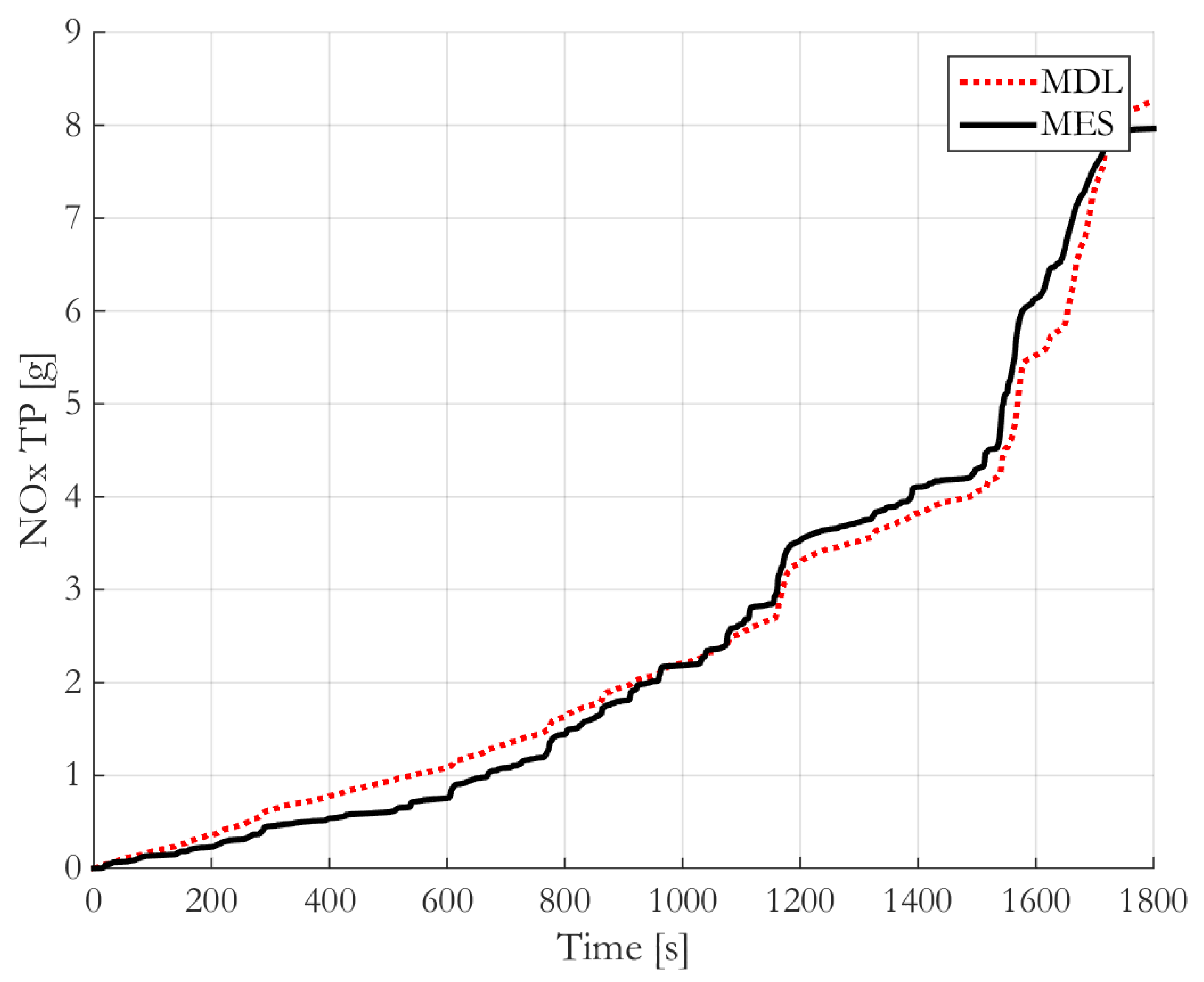
This validation showed a good behavior of the models, even if the strong assumptions inherent to a virtual sensor approach cause non-negligible errors. The estimations of fuel consumption and CO2. Emissions are the most precise with a typical modeling error from 5% to 10% depending on the vehicle and the trip (an example is given in Figure 9). In this case, the main source of error is the estimation of the gearbox ratio in the case of a manual transmission. Among pollutant emissions, the estimation of NOx emissions is the most effective with typical errors ranging from 5% to 20%. For NOx emissions, the most critical situations are short trips with a modern Diesel engine fitted with an after-treatment system highly sensitive to the warm-up duration. CO emissions for gasoline engine and PM for Diesel are the most critical emissions to a model with a typical error of 10% to 25%. Nevertheless, this accuracy is consistent with the level of complexity of the pollutant models.
In the second part of the validation analysis, the objective is to show the model sensitivity to the influence of the type of vehicle, the trip and the driving behavior on the pollutant emissions. The tests were conducted on real-driving data recorded with a smartphone GPS sensor.

3.2.1. Impact of the Driving Behavior

The first interesting result is the significant sensitivity of pollutant emissions to the driving behavior. Figure 10 presents the result of emissions estimated on different speed profiles acquired on a same itinerary with the same vehicle but with different drivers. The speed profile of each driver was recorded during an experimental campaign. On this example, the NOx level of this Euro5 Diesel vehicle can vary by a factor 3 for a fixed trip and vehicle depending only on the driver’s behavior.

3.2.2. Impact of the Trip

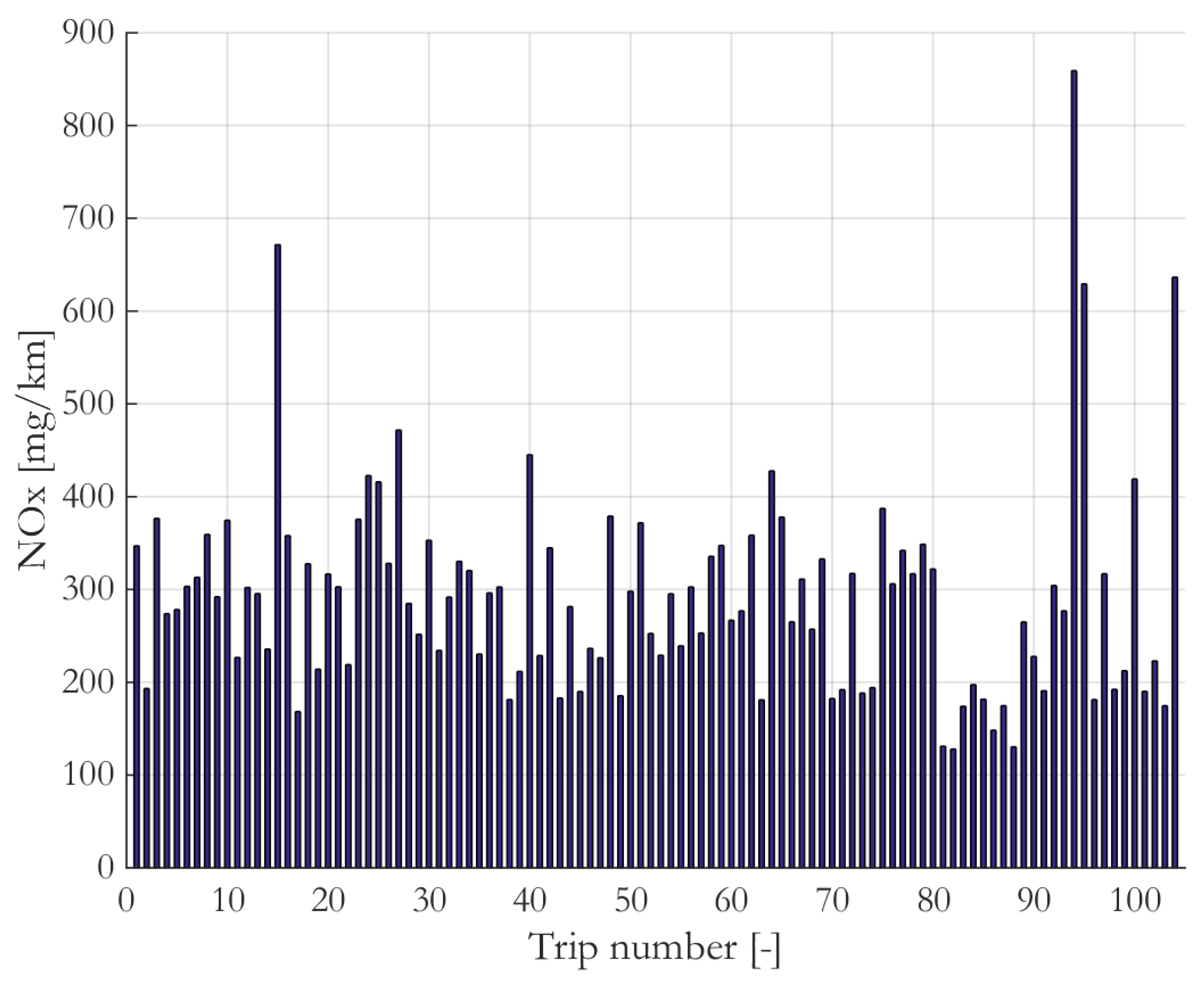
The second interesting result is the sensitivity of the pollutant levels to the trip characteristics. An example is given in Figure 11 showing NOx emissions’ levels on different trips with the same driver and the same vehicle (Euro5 Diesel). The level of pollutants emitted per kilometer vary by a factor 10 depending on the trip length, its contextualization (congestion, signalization, etc.) and its slope profile.

3.2.3. Impact of the Vehicle

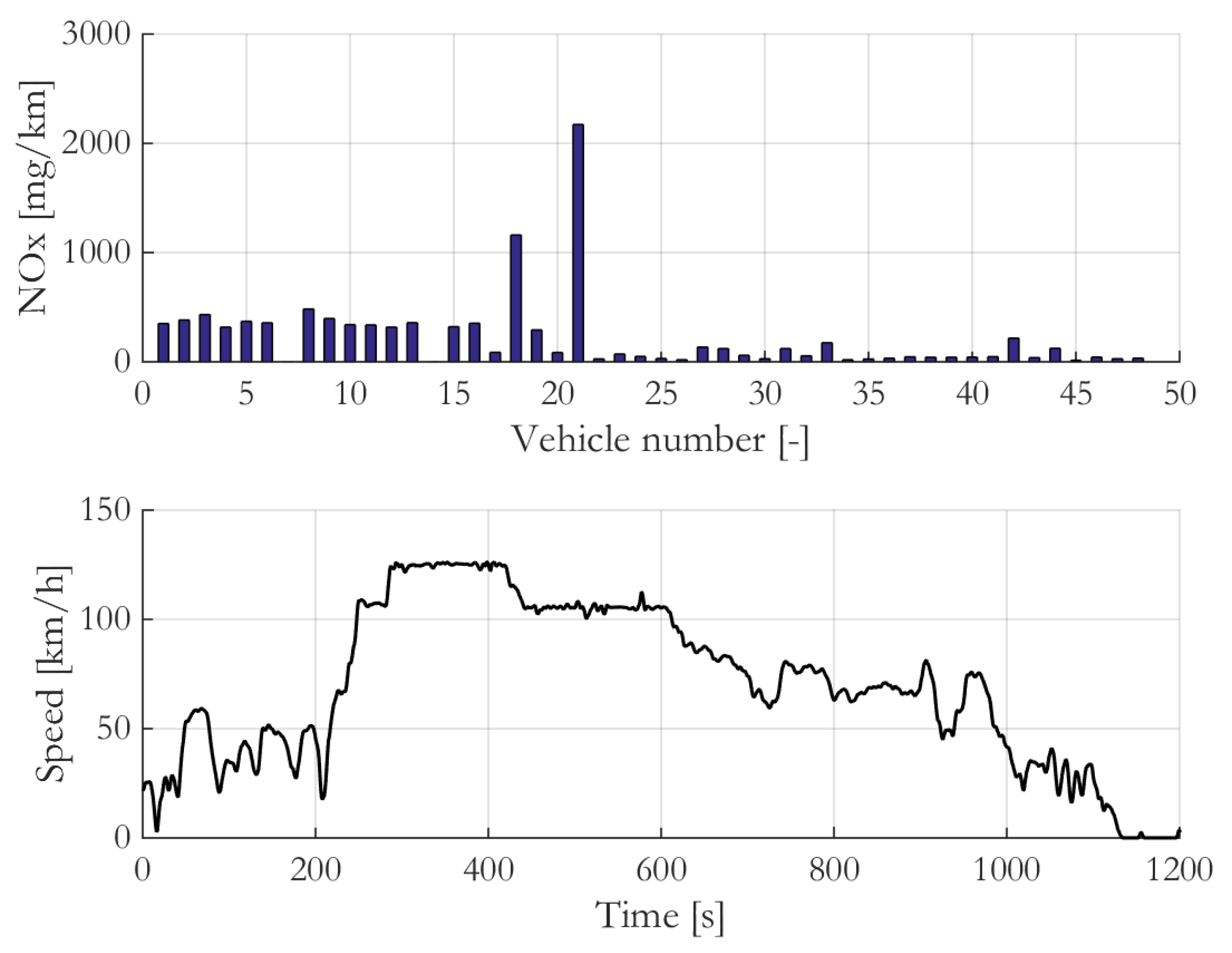
The last result is the analysis of the impact of vehicle and engine characteristics on the pollutant emissions level. Figure 12 gives an example of the NOx emissions for the same speed profile on a sample of 50 vehicles, with diesel and gasoline engines from Euro3 to Euro6. The emissions of recent vehicles are globally lower, but it is interesting to observe that, for some pollutant, the real driving emissions did not decrease as much as the standard level did.

3.3. Microscopic Traffic Emissions

In this third part of the experimental results, our objective is to demonstrate how the previous two blocks of the proposed workflow (i.e., driving behavior model and microscopic emissions model) can be combined to estimate traffic pollutant emissions in a geographical area. In order to do so, as illustrated in Figure 1, additional data sources are required: information about the traffic volume on the road links of the considered area and information about the overall vehicle fleet composition. The results are aimed at showing the added value of the proposed modeling approach in predicting microscopic traffic emissions over the state-of-the-art methods, such as COPERT [32], merely using emission factors per type of vehicle neglecting the dynamic content of the driving behavior. In order to establish this analysis, we benchmark both the proposed model and COPERT against a common reference. Since we do not have a true measurement (PEMS) of pollutant emissions in the experimental area, the reference used in the comparison is the emissions calculated by the microscopic emissions model using as input the Geco air real-world speed profiles recorded on the different links of the road network. Note that the speed recordings in the test area were used only in validation and not in the training of the driving behavior model. In the following, for brevity of presentation, only NOx emissions results will be shown in the figures.
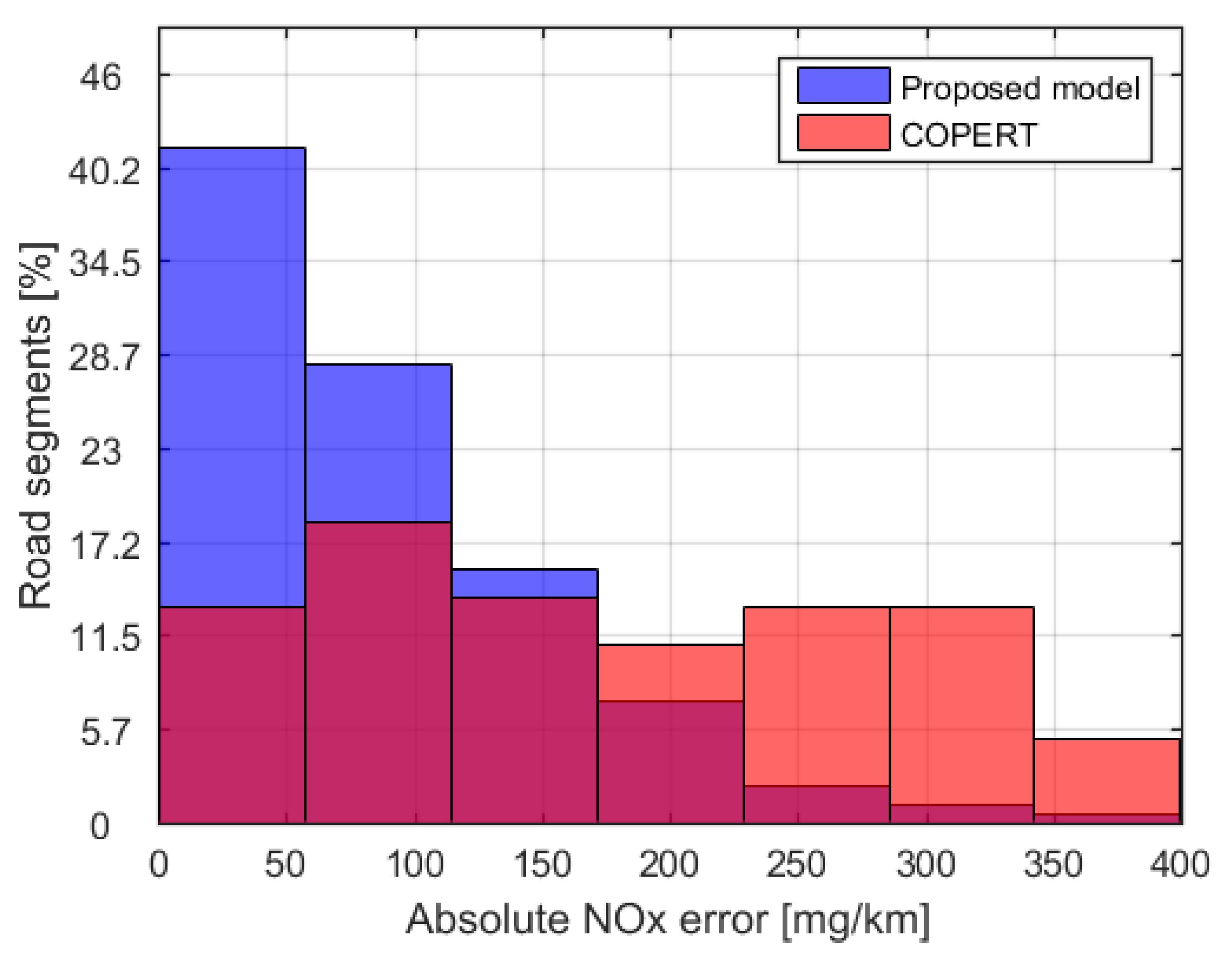
Figure 13 shows histograms of errors in the estimation of NOx emissions, for more than 300 road links. In addition, 75% of the road-links have less than 100 mg/km error with the proposed model, compared to 30% with COPERT. The model mean of the mean absolute error is around 98 mg/km for the proposed model and 219 mg/km for COPERT. The mean absolute error is reduced by more than 55%. A similar error reduction is obtained for the CO2 emissions. The proposed model has a mean absolute error of 21 g/km while it is around 45 g/km for COPERT. This represents respectively 12% and 25% of the mean CO2 emissions for the recorded speed trajectories.
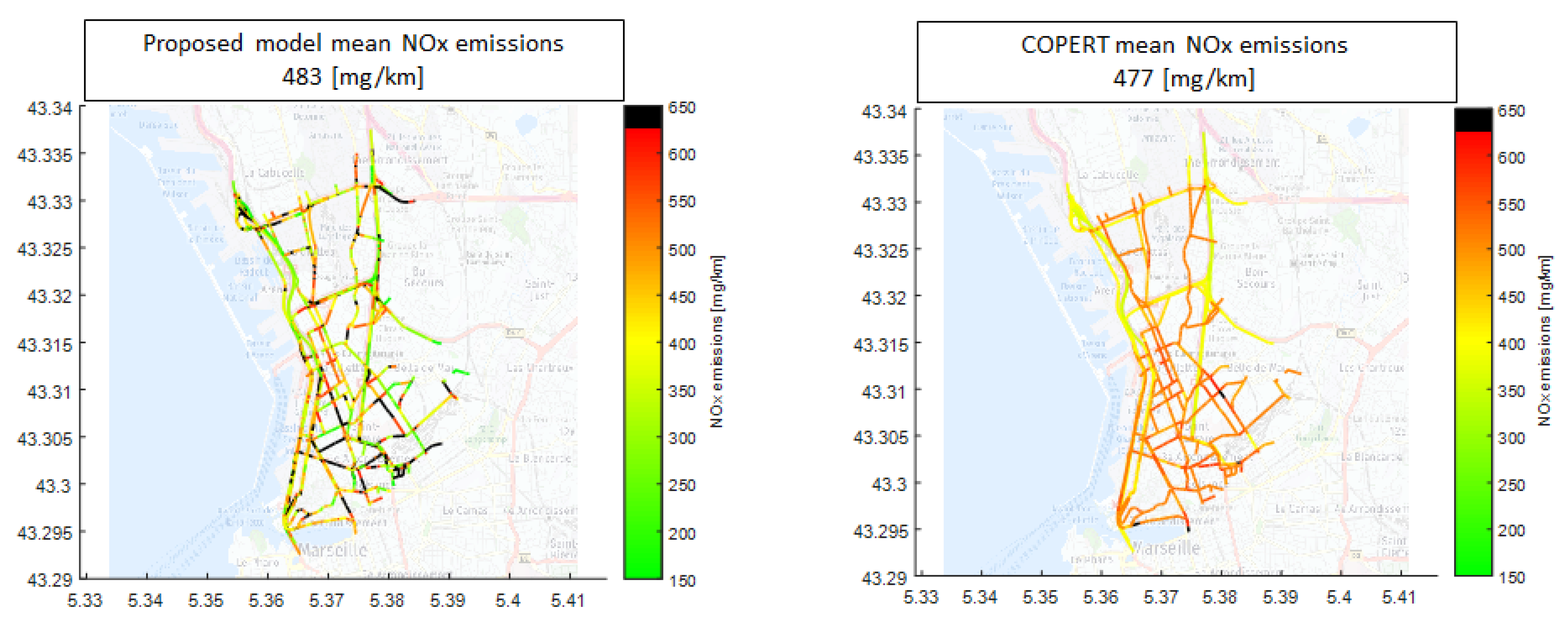
From a qualitative point of view, if we look at the traffic emissions on a map and compare them with the reference emissions (Figure 14), it is possible to see that the proposed models reproduce the true variability of NOx emissions well, as depicted by the reference, while COPERT tends to remain close to the global average by preventing to clearly highlight the critical areas in terms of emissions. Figure 15 illustrates a comparison of maps for vehicle NOx emissions in a neighborhood of Marseilles on all road links. Both COPERT and the proposed models have the same average NOx emissions. However, the proposed model shows more sensitivity: the infrastructure impact on traffic emissions is better taken into account than with the COPERT model.
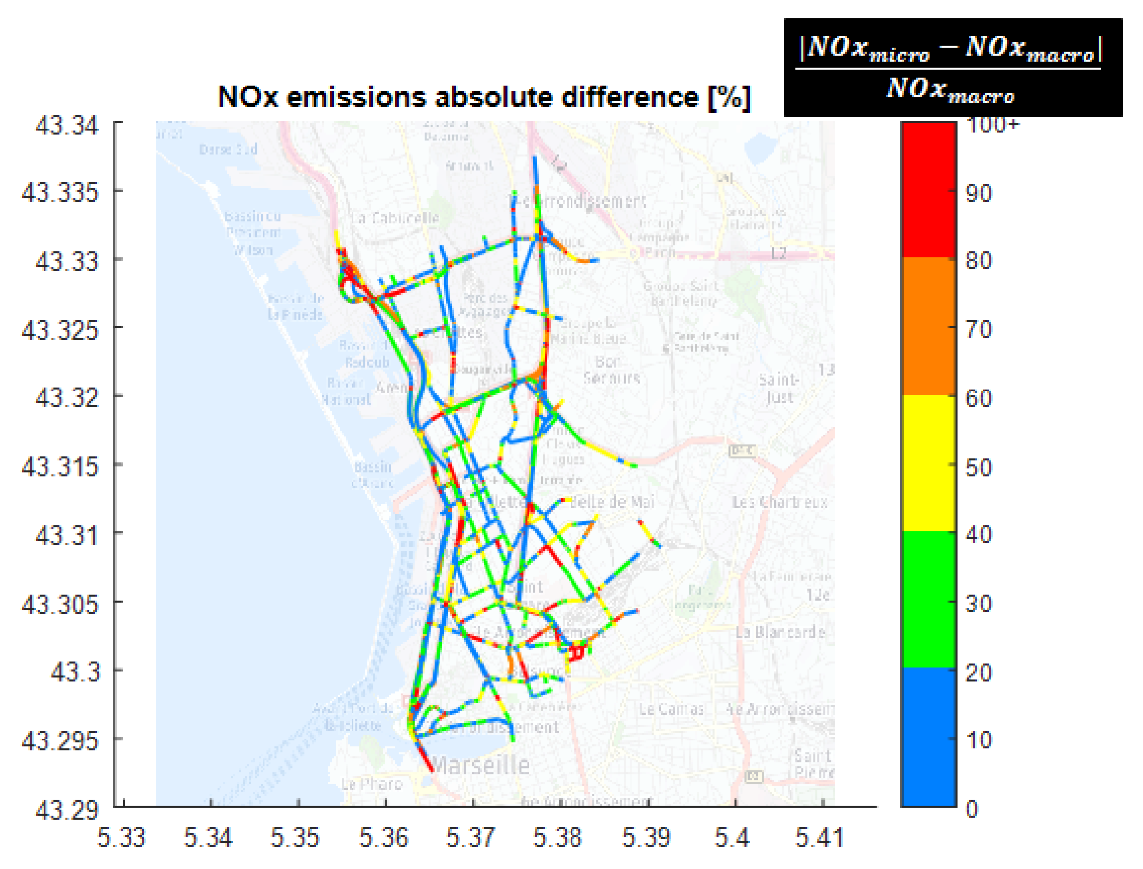
Figure 16 shows the map of relative NOx emission difference between the microscopic and macroscopic approach. Close values of microscopic and macroscopic emissions are indicated by a blue color. A red color means that, on the considered road link, there is more than 80% difference between the two approaches. On average, there is a 40% difference between COPERT and the microscopic model, with 7% of the road links having more than an 80% difference. Results show an increased accuracy of the estimated emissions at a reduced scale. Subsequently, this model could be used to monitor the pollutant emissions level and identify critical areas. Apart from the NOx emissions maps, the model can also be used to generate CO2 and other pollutant emissions maps at a high spatial resolution.
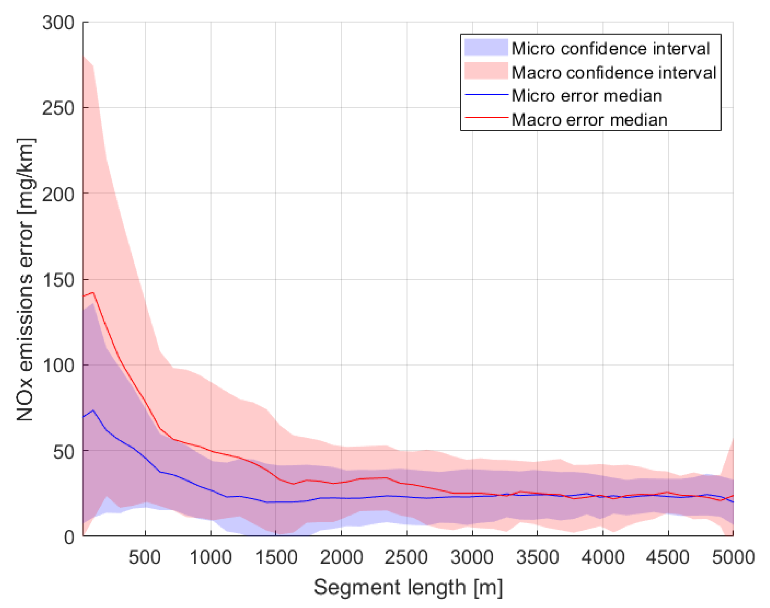
The microscopic and macroscopic approaches show noticeable NOx emissions estimation differences in road segments of different lengths. Figure 17 illustrates the NOx emissions estimation error of both approaches as a function of this length. Those models have been compared to the previously defined reference. For each distance bin, road segments of different lengths have been grouped together in order to obtain at least 50 error estimations. For segment lengths lower than 500 m, the microscopic emission error is reduced by more than 50% in comparison to the macroscopic one. This represents 91% of the road segments in the studied area, for which the mean length is around 55 m. For higher distances, the NOx emission error is reduced, and both approaches converge towards the same NOx emissions error for a segment length around 2700 m. In this case, the spatial resolution is relatively low and the microscopic approach presents no contribution over the macroscopic one.

4. Conclusions

In this work, a complete modeling framework to estimate road traffic microscopic pollutant emissions from easily obtainable macroscopic road topology and traffic information was proposed. The model was trained on a rich data-set of real-world driving speed profiles, but it can be applied on any road network and is able to predict driving behavior and pollutant emissions as a function of simple macroscopic features. The coupling between the road-link-level driving behavior model and the microscopic vehicle emissions model is able to provide high resolution (both in time and space) pollutant emissions’ estimations. Validation results show that the estimation error is significantly reduced, by more than 50%, with respect to well-established macroscopic emissions models, such as COPERT. Furthermore, as a key result, this study shows that the state-of-the-art macroscopic methods to estimate transport-related pollutant emissions are fundamentally inaccurate for spatial resolutions of the order of hundreds of meters, as it is the case in urban road networks. Thus, the proposed methods aim to fill the precision gap for pollutant emissions estimation on relatively small road segments, where the speed variability and the impact of traffic and road infrastructure are more relevant. At the same time, estimation accuracy on longer road segments is not degraded. Finally, the proposed modeling framework may also be used as a more precise road-transport emissions source for atmospheric dispersion and air quality models. Both high-resolution pollutant emissions and pollutants concentration could then be used by cities to detect critical areas and/or infrastructure elements negatively affecting local air quality.

Author Contributions

All the authors contributed equally to the conceptualization, methodology, formal analysis, investigation, validation, visualization and writing. Software, M.L. and L.T.; supervision and project administration, G.D.N. and L.T.; funding acquisition, L.T. All authors have read and agreed to the published version of the manuscript.

Funding

This research was funded by ADEME (French Environment and Energy Management Agency); AIRMES project, PRIMEQUAL 2018, Grant No. 1866C0013.

Institutional Review Board Statement

Not applicable.

Informed Consent Statement

Not applicable.

Acknowledgments

The authors would like to thank the partners of the project, AtmoSud and ARIA Technologies, for providing traffic volume data in the test area, as well as valuable feedback for the interpretation of the results.

Conflicts of Interest

The authors declare no conflict of interest. The funders had no role in the design of the study; in the collection, analyses, or interpretation of data; in the writing of the manuscript, or in the decision to publish the results.

References

  1. CITEPA. Gaz à effet de Serre et Polluants Atmosphériques. Bilan des émissions en France de 1990 à 2018; Technical Report; CITEPA: Paris, France, 2020. [Google Scholar]
  2. Dalton, G.; de la Peña, E.; Vassallo, J.M.; Acciaro, M. Transport Infrastructure; Technical Report; European Commission: Brussels, Belgium, 2017. [Google Scholar]
  3. Höglund, P.G.; Niittymäki, J. Estimating vehicle emissions and air pollution related to driving patterns and traffic calming. In Submitted Paper for the Conference Urban Transport Systems, Lund, Sweden; Lund University: Lund, Sweden, 1999; Volume 7. [Google Scholar]
  4. Van Lint, J.; Van der Zijpp, N. Improving a travel-time estimation algorithm by using dual loop detectors. Transp. Res. Rec. 2003, 1855, 41–48. [Google Scholar] [CrossRef]
  5. Treiber, M.; Helbing, D. An adaptive smoothing method for traffic state identification from incomplete information. In Interface and Transport Dynamics; Springer: Berlin/Heidelberg, Germany, 2003; pp. 343–360. [Google Scholar]
  6. Chu, L.; Oh, S.; Recker, W. Adaptive Kalman filter based freeway travel time estimation. In Proceedings of the 84th TRB Annual Meeting, Washington, DC, USA, 9–13 January 2005. [Google Scholar]
  7. Min, W.; Wynter, L. Real-time road traffic prediction with spatio-temporal correlations. Transp. Res. Part C Emerg. Technol. 2011, 19, 606–616. [Google Scholar] [CrossRef]
  8. Newell, G.F. A simplified theory of kinematic waves in highway traffic, part I: General theory. Transp. Res. Part B Methodol. 1993, 27, 281–287. [Google Scholar] [CrossRef]
  9. Smulders, S. Control of freeway traffic flow by variable speed signs. Transp. Res. Part B Methodol. 1990, 24, 111–132. [Google Scholar] [CrossRef]
  10. Fellendorf, M.; Vortisch, P. Microscopic traffic flow simulator VISSIM. In Fundamentals of Traffic Simulation; Springer: Berlin/Heidelberg, Germany, 2010; pp. 63–93. [Google Scholar]
  11. Yang, Q.; Koutsopoulos, H.N. A microscopic traffic simulator for evaluation of dynamic traffic management systems. Transp. Res. Part C Emerg. Technol. 1996, 4, 113–129. [Google Scholar] [CrossRef]
  12. Effa, R.C.; Larsen, L. Development of real-world driving cycles for estimating facility-specific emissions from light-duty vehicles. In Proceedings of the Air and Waste Management Association Annual Specialty Conference Emission Inventory: Perception and Reality, Pasadena, CA, USA, 18–20 October 1993. [Google Scholar]
  13. Lin, J.; Niemeier, D.A. Estimating regional air quality vehicle emission inventories: Constructing robust driving cycles. Transp. Sci. 2003, 37, 330–346. [Google Scholar] [CrossRef] [Green Version]
  14. Andrieu, C. Modélisation Fonctionnelle de Profils de Vitesse en lien Avec l’infrastructure et méthodologie de Construction d’un profil agrégé. Ph.D. Thesis, Paul Sabatier University, Toulouse, France, 6 January 2013. [Google Scholar]
  15. Wolfermann, A.; Alhajyaseen, W.K.; Nakamura, H. Modeling speed profiles of turning vehicles at signalized intersections. In Proceedings of the 3rd International Conference on Road Safety and Simulation RSS2011, Transportation Research Board TRB, Indianapolis, IN, USA, 14–16 September 2011. [Google Scholar]
  16. Minett, C.F.; Salomons, A.M.; Daamen, W.; Van Arem, B.; Kuijpers, S. Eco-routing: Comparing the fuel consumption of different routes between an origin and destination using field test speed profiles and synthetic speed profiles. In Proceedings of the 2011 IEEE Forum on Integrated and Sustainable Transportation Systems, Vienna, Austria, 29 June–1 July 2011; pp. 32–39. [Google Scholar]
  17. De Nunzio, G.; Thibault, L.; Sciarretta, A. Model-based eco-routing strategy for electric vehicles in large urban networks. In Comprehensive Energy Management—eco Routing & Velocity Profiles; Springer: Berlin/Heidelberg, Germany, 2017; pp. 81–99. [Google Scholar]
  18. Laureshyn, A.; Åström, K.; Brundell-Freij, K. From speed profile data to analysis of behaviour: Classification by pattern recognition techniques. IATSS Res. 2009, 33, 88–98. [Google Scholar] [CrossRef] [Green Version]
  19. Laraki, M.; De Nunzio, G.; Thibault, L. Vehicle speed trajectory estimation using road traffic and infrastructure information. In Proceedings of the IEEE 23rd International Conference on Intelligent Transportation Systems, Rhodes, Greece, 20–23 September 2020. [Google Scholar]
  20. Pelkmans, L.; Debal, P. Comparison of on-road emissions with emissions measured on chassis dynamometer test cycles. Transp. Res. Part D Transp. Environ. 2006, 11, 233–241. [Google Scholar] [CrossRef]
  21. Real-Time on-road Vehicle Exhaust Gas Modular Flowmeter and Emissions Reporting System. U.S. Patent 6,148,656, 21 November 2000.
  22. Gao, J.; Tian, G.; Sorniotti, A.; Karci, A.E.; Di Palo, R. Review of thermal management of catalytic converters to decrease engine emissions during cold start and warm up. Appl. Therm. Eng. 2019, 147, 177–187. [Google Scholar] [CrossRef]
  23. Gao, J.; Chen, H.; Dave, K.; Chen, J.; Jia, D. Fuel economy and exhaust emissions of a diesel vehicle under real traffic conditions. Energy Sci. Eng. 2020, 8, 1781–1792. [Google Scholar] [CrossRef]
  24. Liu, H.; Chen, X.; Wang, Y.; Han, S. Vehicle Emission and Near-Road Air Quality Modeling for Shanghai, China: Based on Global Positioning System Data from Taxis and Revised MOVES Emission Inventory. Transp. Res. Rec. 2013, 2340, 38–48. [Google Scholar] [CrossRef]
  25. Sentoff, K.M.; Aultman-Hall, L.; Holmén, B.A. Implications of driving style and road grade for accurate vehicle activity data and emissions estimates. Transp. Res. Part D Transp. Environ. 2015, 35, 1756188. [Google Scholar] [CrossRef]
  26. Ma, X.; Lei, W.; Andréasson, I.; Chen, H. An Evaluation of Microscopic Emission Models for Traffic Pollution Simulation Using On-board Measurement. Environ. Model. Assess. 2012, 17, 375–387. [Google Scholar] [CrossRef]
  27. Chen, K.; Yu, L. Microscopic Traffic-Emission Simulation and Case Study for Evaluation of Traffic Control Strategies. J. Transp. Syst. Eng. Inf. Technol. 2007, 7, 93–99. [Google Scholar] [CrossRef]
  28. Badin, A.L.; Clavel, A.; Vittoz, T.; Sorand, C.; Lejri, D.; Leclercq, L.; Olny, X. Combining microscopic traffic modelling and 3 pollutant emission modellings to assess modifications of traffic supply and demand. J. Earth Sci. Geotech. Eng. 2017, 7, 175–190. [Google Scholar]
  29. Nam, E.K.; Gierczak, C.A.; Butler, J.W. A Comparison of Real-World and Modeled Emissions Under Conditions of Variable Driver Aggressiveness. 2003. Available online: https://silo.tips/download/a-comparison-of-real-world-and-modeled-emissions-under-conditions-of-variable-dr (accessed on 30 November 2020).
  30. Hausberger, S. Simulation of Real World Vehicle Exhaust Emissions; VKM-THD Mitteilungen Technical University Graz: Graz, Austria, 2003; Volume 82. [Google Scholar]
  31. Geco Air. Available online: https://www.gecoair.fr/home_en/ (accessed on 30 November 2020).
  32. Ntziachristos, L.; Gkatzoflias, D.; Kouridis, C.; Samaras, Z. COPERT: A European road transport emission inventory model. In Information Technologies in Environmental Engineering; Springer: Berlin/Heidelberg, Germany, 2009; pp. 491–504. [Google Scholar]
  33. HERE Maps. Available online: https://www.here.com/ (accessed on 30 November 2020).
  34. Van Hieu, D.; Meesad, P. Fast K-Means Clustering for Very Large Datasets Based onMapReduce Combined with a New Cutting Method. Available online: http://link.springer.com/chapter/10.1007%2F978-3-319-11680-8_23 (accessed on 30 November 2020).
  35. Kaufman, L.; Rousseeuw, P.J. Finding Groups in Data: An Introduction to Cluster Analysis; John Wiley & Sons: Hoboken, NJ, USA, 2009; Volume 344. [Google Scholar]
  36. Breiman, L. Random forests. Mach. Learn. 2001, 45, 5–32. [Google Scholar] [CrossRef] [Green Version]
  37. Bengio, Y.; Grandvalet, Y. No unbiased estimator of the variance of k-fold cross-validation. J. Mach. Learn. Res. 2004, 5, 1089–1105. [Google Scholar]
  38. Alix, G.; Dabadie, J.; Font, G. An ICE Map Generation Tool Applied to the Evaluation of the Impact of Downsizing on Hybrid Vehicle Consumption.; SAE International: Warrendale, PA, USA, 2015. [Google Scholar]
  39. Gärtner, U.; Hohenberg, G.; Daudel, C.; Oelschlegel, H. Development and Application of a Semi-Empirical NOx Model to Various HD Diesel Engines. In Thermo- and Fluid Dynamic Processes in Diesel Engines 2; Springer: Berlin/Heidelberg, Germany, 2004; pp. 285–312. [Google Scholar]
  40. Depcik, C.; Assanis, D. One-dimensional automotive catalyst modeling. Prog. Energy Combust. Sci. 2005, 31, 308–369. [Google Scholar] [CrossRef]
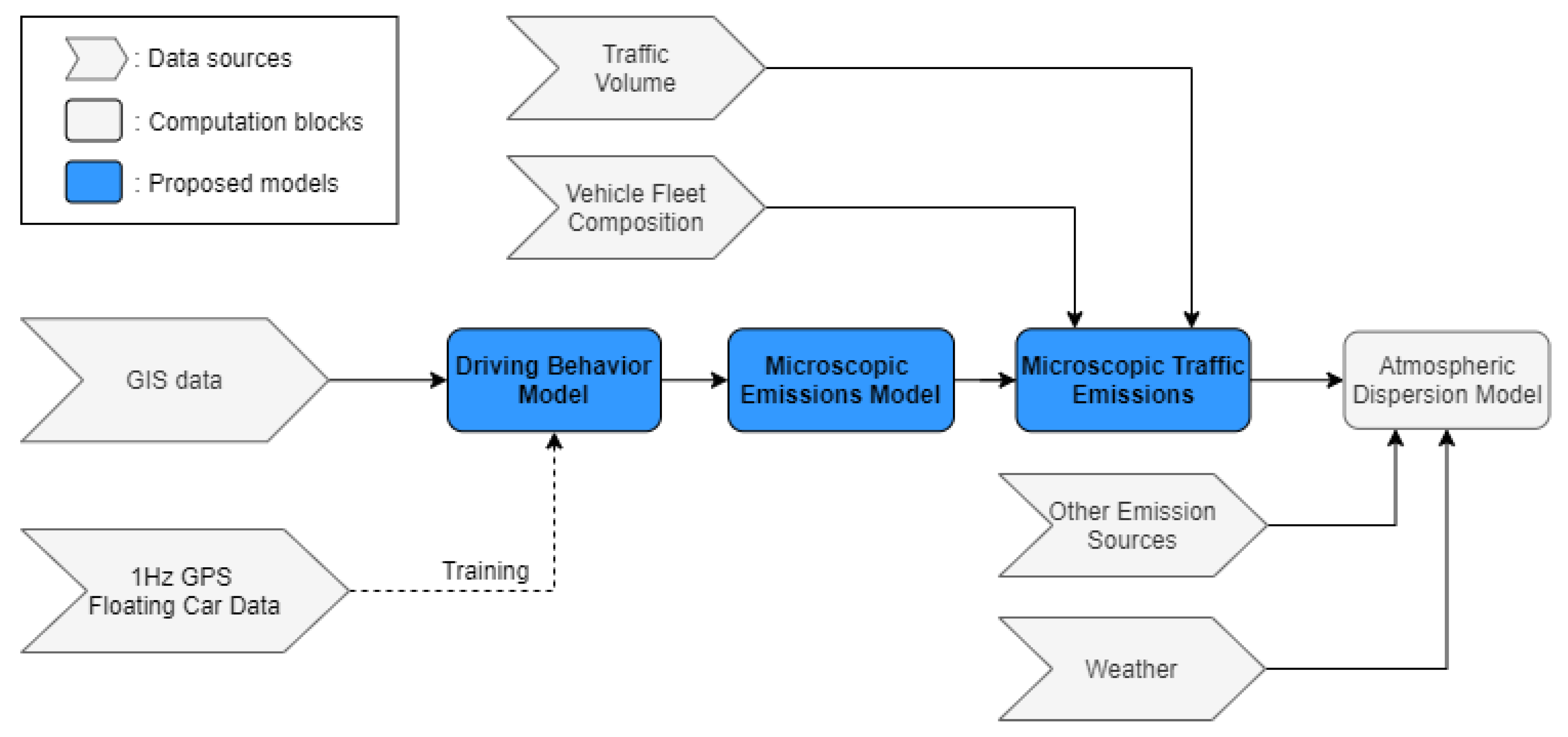
Figure 1. Illustration of the overall approach to translate macroscopic road information into road traffic environmental impact. This work focuses on the central blocks computing the microscopic vehicle emissions from only macroscopic available data.
Atmosphere 12 00053 g001
Figure 2. Illustration of the cascaded driving behavior model.
Atmosphere 12 00053 g002
Figure 3. Proposed decision tree, nine categories are identified.
Atmosphere 12 00053 g003
Figure 4. Vehicle pollutant emissions model scheme.
Atmosphere 12 00053 g004
Figure 5. Implicit algorithm applied to compute physical quantities.
Atmosphere 12 00053 g005
Figure 6. Example of after-treatment submodels for a Diesel Euro6 exhaust line.
Atmosphere 12 00053 g006
Figure 7. Constructed speed trajectory error comparison between deterministic and stochastic approach for stop cases.
Atmosphere 12 00053 g007
Figure 8. Comparison between constructed and measured vehicle speed trajectories for a road link.
Atmosphere 12 00053 g008
Figure 9. Comparison between the estimates (red curve) and experimental measurements (black curve) of Fuel Consumption (left figure) and NOx emissions (right figure) for a Diesel Euro5 on the WLTC driving cycle.
Atmosphere 12 00053 g009
Figure 10. Example of NOx sensitivity on a sample of 26 drivers, on a same trip with the same vehicle (Diesel Euro5).
Atmosphere 12 00053 g010
Figure 11. Example of NOx sensitivity on a sample of 104 trips, with the same driver and same vehicle (Diesel Euro5).
Atmosphere 12 00053 g011
Figure 12. Example of NOx sensitivity to the vehicle, on the same real-world speed profile (i.e., same trip and same driver).
Atmosphere 12 00053 g012
Figure 13. Comparison of errors between the proposed model and the COPERT approach.
Atmosphere 12 00053 g013
Figure 14. Map of NOx emissions in Marseilles, France, and comparison of the estimate with the reference and COPERT. Only road segments with sufficient measured driving data are displayed.
Atmosphere 12 00053 g014
Figure 15. COPERT vs. proposed model. NOx emissions maps comparison in Marseilles, France. Colorbar color scale is black at 630 mg/km. Above this value, the road-link is considered a high emitter. The black color saturation is used to identify more easily critical road links.
Atmosphere 12 00053 g015
Figure 16. NOx emissions relative difference between the proposed model and COPERT.
Atmosphere 12 00053 g016
Figure 17. Microscopic and macroscopic NOx estimation errors as a function of the road segment length.
Atmosphere 12 00053 g017
Table 1. Macroscopic features for the definition of categories.
Feature Description
Congestion level
Traffic light
Stop sign
Yield sign
Road network hierarchy
Road link curvature
Table 2. Clustering features for the identification of driving behaviors.
Feature Description
Mean speed
Percentage of null speed
75% percentile of speed
Minimum speed
Sum of positive acceleration
Sum of negative acceleration
Difference between initial and final speed
Table 3. Features used as inputs of the RF algorithm.
FeatureDescription
N l Number of lanes in the road link
V O t Origin road link traffic speed
V t Center road link traffic speed
V D t Destination road link traffic speed
V n Nominal speed
L s road link length
α s Slope angle
α c Curvature angle
N i Number of adjacent origin road links
N f Number of adjacent destination road links
Table 4. Errors between modeled and measured speed trajectories for the validation case (Marseilles, France).
Error v i v m v f
Mean absolute error2.22 km/h2.26 km/h2.32 km/h
Relative error8 %8.5 %9 %
Publisher’s Note: MDPI stays neutral with regard to jurisdictional claims in published maps and institutional affiliations.