Article

Future Projections and Uncertainty Assessment of Precipitation Extremes in the Korean Peninsula from the CMIP6 Ensemble with a Statistical Framework

1
Department of Mathematics and Statistics, Chonnam National University, Gwangju 61186, Korea
2
Department of Atmospheric Science, Kongju National University, Gongju 32588, Korea
3
National Institute of Meteorological Sciences, Seogwipo 63568, Korea
4
Department of Atmospheric and Environmental Sciences, Gangneung-Wonju National University, Gangneung 25457, Korea
5
Department of Earth Science Education, Kyungpook National University, Daegu 41566, Korea
*
Author to whom correspondence should be addressed.
Atmosphere 2021, 12(1), 97; https://doi.org/10.3390/atmos12010097
Submission received: 24 November 2020 / Revised: 5 January 2021 / Accepted: 6 January 2021 / Published: 11 January 2021

Abstract

:
Scientists occasionally predict projected changes in extreme climate using multi-model ensemble methods that combine predictions from individual simulation models. To predict future changes in precipitation extremes in the Korean peninsula, we examined the observed data and 21 models of the Coupled Model Inter-Comparison Project Phase 6 (CMIP6) over East Asia. We applied generalized extreme value distribution (GEVD) to a series of annual maximum daily precipitation (AMP1) data. Multivariate bias-corrected simulation data under three shared socioeconomic pathway (SSP) scenarios—namely, SSP2-4.5, SSP3-7.0, and SSP5-8.5—were used. We employed a model weighting method that accounts for both performance and independence (PI-weighting). In calculating the PI-weights, two shape parameters should be determined, but usually, a perfect model test method requires a considerable amount of computing time. To address this problem, we suggest simple ways for selecting two shape parameters based on the chi-square statistic and entropy. Variance decomposition was applied to quantify the uncertainty of projecting the future AMP1. Return levels spanning over 20 and 50 years, as well as the return periods relative to the reference years (1973–2010), were estimated for three overlapping periods in the future, namely, period 1 (2021–2050), period 2 (2046–2075), and period 3 (2071–2100). From these analyses, we estimated that the relative increases in the observations for the spatial median 20-year return level will be approximately 18.4% in the SSP2-4.5, 25.9% in the SSP3-7.0, and 41.7% in the SSP5-8.5 scenarios, respectively, by the end of the 21st century. We predict that severe rainfall will be more prominent in the southern and central parts of the Korean peninsula.

1. Introduction

Heavy precipitation can have cascading effects on communities, infrastructure, agriculture, and livestock, as well as on economically and culturally important natural ecosystems. For example, extreme rain events can result in costly damage to wastewater treatment plants, culverts, and roads. Extreme precipitation can result in landslides and floods, accompanied with a loss of life and the deterioration of infrastructure. Thus, understanding and projecting heavy rainfall is of significant importance to climate change impact, adaptation, and vulnerability assessments.
Numerous studies have reported that extreme precipitation events have become more frequent during the last century, and are occurring even more often over the 21st century ([1,2,3,4,5,6,7], for example). A simplified and major reason for more frequent extreme rainfall is the following: Warming conditions mean more evaporation, which leads to more water vapor in the air. When rain-triggering conditions are favorable, more saturated air leads to heavier precipitation [8,9]. This has been the case across some areas of the world during the last century [10]. For example, heavy daily rainfall has accounted for an increased proportion of total annual rainfall over an increasing fraction of the Australian continent since the 1970s ([11], Section 4.2.3). The average annual rainfall has already increased by nearly 50% over parts (including the Netherlands, Belgium, and Luxembourg) of northern Europe [12]. This trend is likely to be accelerated with increased global warming over the 21st century [10,12]. Some studies have projected that global warming leads to a higher intensity of precipitation and longer dry periods, for example, in Europe and Asia [13,14,15,16]. Seemingly paradoxically, as written by Mann and Kump [12], “While many regions are likely to become drier, scientists predict that even in those regions individual rainfall or snowfall events will become more intense, although longer dry spells will separate them.”
Extreme rainfall occurs frequently over the Korean peninsula during the warm season from June through September, in association with synoptic disturbances, typhoons, or convective changes within the air masses over the region. Previous studies [17,18,19] have reported an increase in observed extreme precipitation in Korea. Lee et al. [20] predicted that the increasing changes in the future heavy rainfall across East Asia appear more distinctly in Korea at a local scale, which indicates a higher sensitivity of the Korean peninsula to global warming. It is thus crucial to project and assess the changes in extreme precipitation events in Korea under different scenarios.
Some authors [21,22,23,24,25,26,27] have predicted increasing changes in future extreme rainfall over Korea by using a single model, ensembles of regional climate models, or multiple Coupled Model Inter-Comparison Project Phase 5 (CMIP5) models. In this study, we update the previous studies based on the multiple CMIP6 models under the three shared socioeconomic pathway (SSP) scenarios—namely, SSP2-4.5, SSP3-7.0, and SSP5-8.5 [28].
Studies on the projection of future climate change have used ensembles of multiple climate simulations. Multi-model ensemble (MME) methods of climatic projection have been proven to improve upon the systematic bias and to have fewer of the general limitations that are typically associated with single simulation models. Among the many ensemble methods, model weighting or averaging is typically employed ([29,30,31], for example). Model averaging is a statistical method in which unequal or equal weights are assigned to those models. Despite some arguments, the equal weighting or “model democracy” [30] has been criticized because it does not take into account the performance, uncertainty, and independency of each model in constructing an MME ([32,33,34], for example).
One typical unequal weighting scheme involves giving more weights to those models that are more skillful and realistic for a specific process or application. This performance-based weighting method and its variants, including Bayesian model averaging (BMA), have been employed in many different studies. It has improved the accuracy of the projections and reduced the prediction uncertainty. However, it has been reported that only a few models often exhibit extremely high weights, and most others have very low weights [27,35]. This phenomenon may be because some models are more fit to the observations for given applications than others, and thus, they receive extremely high weights in a multi-model estimate of change [36]. Such an aggressive weighting based on performance will only be dangerous in the sense of an overfitting when observational uncertainty is large, and thus, it is not robust in quantifying the uncertainty.
In addition to the performance, some researchers have considered other criteria, such as model convergence [37], model independency [32,38,39,40], and a semi-performance measure [41]. A weighting scheme that accounts for both the independence and performance simultaneously is called the PI-weighting. In this study, we employ PI-weighting to robustly quantify uncertainty in an MME. In calculating the PI-weights, considering only one or two climate variables over a relatively small area can lead to an overfitting problem [36,40]. To avoid this problem, we thus consider five climate variables over East Asia, while our focus is the annual maximum daily precipitation (AMP1) over the Korean peninsula.
In applying the PI-weighting, we have to determine two shape parameters that control the strength of the weights. One way to select the shape parameters is a leave-one-out perfect model test [36,40], but it requires a huge amount of computing time. To overcome this computational problem, we suggest simple ways to determine these parameters based on the entropy and p-values of the chi-square statistic.
The remainder of this paper is structured as follows. The data construction and numerical models are described in Section 2. The statistical methods are briefly mentioned in Section 3. Section 4 describes the PI-weighting with the computational details, including simple ways for determining the shape parameters. The results of the model weights and projected future changes are presented in Section 5 and Section 6, respectively. Section 7 describes the results of an uncertainty assessment and projection by latitude based on an analysis of variance. In Section 8, relative improvement of the PI-weighted method over the simple average is quantified using the skill score and prediction variance. Discussions are then given in Section 9, followed by a summary of the paper in Section 10. Details including technical specifics, tables, and figures are provided in the accompanying Supplementary Material (hereafter referred to as the Supplementary Materials) file.

2. Data and Simulation Models

We consider five climate variables over East Asia to avoid overfitting in calculating the PI-weights, while our focus is the annual maximum daily rainfall (AMP1) over the Korean peninsula in this study. Table 1 lists five climate variables.
Consecutive wet days and dry days are defined as consecutive days with daily precipitation of ≥1 and <1 mm, respectively [42,43]. Table S1 in the accompanying Supplementary Materials lists the 21 CMIP6 climate models used in this study. The considered scenarios are shared socioeconomic pathways SSP2-4.5, SSP3-7.0, and SSP5-8.5 [28]. Hereafter, we shorten the scenario names to SSP2, SSP3, and SSP5, although we use both versions interchangeably. Three overlapping periods are considered for future data, namely, period 1 (2021–2050), period 2 (2046–2075), and period 3 (2071–2100), abbreviated by P1, P2, and P3 in this study.
To re-grid the common grid points of 1 × 1 , the iterative Barnes interpolation scheme [44] was employed for the observations and simulation data from the 21 models for each of five climate variables. The Barnes technique produces a rainfall field on a regular grid from irregularly distributed rainfall observation stations.
East Asia (EA) is considered by many authors (e.g., [4,14,15,45,46]) to be one of the regions most vulnerable to future increases in extreme weather and climate under global warming. For example, projected changes in extreme precipitation indices over the Asian monsoon domain are larger than over other monsoon domains, indicating the strong sensitivity of Asian monsoons to global warming [47].
Figure 1 depicts maps of EA and the Korean peninsula (KP) showing the observations sites and 1180 points over 1 × 1 grids. The observations for the 38-year reference period (1973–2010) were obtained from the Meteorological Administrations of China, Japan, and Korea. In China, observations from 726 stations were used [48] to construct data for 1056 grids. In Japan, observations from 1325 sites were used [49] to construct data for 78 grids.
There are 64 and 27 observation stations in South and North Korea, respectively [50]. Because the 27 stations (black circles in Figure 1) in North Korea are too sparse, re-gridding using Barnes interpolation may not capture the locality of severe rainfall there. For a better re-gridding in North Korea, we used the Asian Precipitation Highly Resolved Observational Data Integration Towards Evaluation (APHRODITE) reanalysis data [51] as auxiliary information. However, the AMP1 in APHRODITE has serious bias in its mean and variance, as shown in Figure S1. We thus correct it using nearby observations using the quantile mapping technique [52]. Examples of time series plots of the observations, APHRODITE data, and the bias-corrected APHRODITE data near the observational stations are shown in Figure S1. Then, the bias-corrected APHRODITE data and the observations at stations were used together for better interpolation in re-gridding. On the right side of Figure 1, the map of the KP shows the spatial distribution of 91 rainfall observation stations, the 80 APHRODITE grid points in North Korea, and the final 46 grids used in this study.

3. Methods

3.1. Generalized Extreme Value Distribution

The generalized extreme value distribution (GEVD) is widely used to analyze extreme univariate values. The three types of extreme value distributions are sub-classes of GEVD. The cumulative distribution function of the GEVD is as follows:
G ( x ) = e x p 1 + ξ x μ σ 1 / ξ ,
when 1 + ξ ( x μ ) / σ > 0 , where μ , σ , and ξ are the location, scale, and shape parameters, respectively. The particular case for ξ = 0 in Equation (1) is the Gumbel distribution, whereas the cases for ξ > 0 and ξ < 0 are known as the Fréchet and the negative Weibull distributions, respectively [53].
It can be helpful to describe the changes in extremes in terms of the changes in extreme quantiles. These are obtained by inverting the following (1): z p = μ σ ξ [ 1 { l o g ( 1 p ) } ξ ] , where G ( z p ) = 1 p . Here, z p is known as the return level associated with the return period 1 / p because level z p is expected to be exceeded, on average, once every 1 / p years [53]. For example, a 20-year return level is computed as the 95th percentile of the fitted GEVD and a 50-year return level as the 98th percentile. Conversely to the above, the return period T ( z ) = 1 / p for the given value z is obtained by calculating p = 1 G ( z ) . For the given value z, T ( z ) is sometimes called the expected waiting time, and the value p = 1 G ( z ) is referred to as the exceedance probability of z.
Assuming the data approximately follow a GEVD, the parameters can be estimated by the maximum likelihood method [53,54] or the method of L-moment estimation. The L-moment estimator is more efficient than the maximum likelihood estimator in small samples for typical shape parameter values [55]. The L-moment method is employed in this study using the “lmom” package in R [56] because a relatively small number of samples are analyzed for each comparison period. Moreover, the formulae used to obtain the L-moment estimator are simple compared to those for obtaining the maximum likelihood estimator, which needs an iterative optimization until convergence.

3.2. Bias Correction

Although simulations from climate or meteorological models provide significant information, the simulated data are associated with potential biases in that their statistical distribution differs from the distribution of the observations. This is partly because of unpredictable internal variability that differs from the observations, and because global climate models (GCMs) have a very low spatial resolution for being employed directly in most impact models [57,58]. For example, in GCM precipitation fields, the bias may be due to errors in convective parameterizations and unresolved subgrid-scale orography [59]. Bias-correction (BC) methods are commonly applied to transform the simulated data into new data with no or fewer statistical biases with respect to an observed time series. In this study, future simulation outputs are bias corrected to compute the intensity of extreme rainfall.
To correct the model outputs more efficiently by taking account of the dependency among variables or nearby grids, several multivariate BC methods have recently been proposed. In this study, we chose the multivariate bias correction (MBC) method by Cannon [59] among the many available BC methods [52]; it is a multivariate extension of quantile delta mapping (QDM). QDM has an advantage of preserving the approximate trends of the model data. In this study, the MBC is applied to the five climate variables provided in Table 1 to take into account the dependency among these variables. The MBC is applied one time to the future simulation data for all periods (2021–2100) based on the historical information, not for each period separately. More details are provided in the Supplementary Materials.

4. Weighting Method for Ensembles

4.1. Performance and Independence Weighting

Knutti et al. [39] argued that the growing number of models with different characteristics and considerable interdependence finally justifies abandoning a strict model democracy. They provided at least five reasons for why PI-weighting is required. Brunner et al. [36] illustrated that PI-weighting leads to an increase in the investigated skill score for temperature and precipitation while minimizing the probability of overfitting (or overconfidence).
As the basic idea of PI-weighting, models that agree poorly with observations for a selected set of diagnostics receive less weight, as do models that largely duplicate existing models [39]. Weights are calculated for each model based on a combination of the distance D i (informing the performance) and the model similarity S i j (informing the dependence):
w i = e x p ( D i σ D ) 1 + j i M e x p ( S i j σ S ) ,
with the total number of model runs M and the shape parameters σ D and σ S . The weights are normalized such that their sum equals 1. The details in computing the performance distance D i are given in the Supplementary Materials.
The numerator represents the modeling skill when using a Gaussian weighting, where the weight decreases exponentially the farther away a model is from the observations. The denominator is the “effective repetition of a model” [32] and is intended to account for the model interdependency [39]. The details in computing the distance S i j are given in the next subsection.
The shape parameters define the strength of the weighting and the relative importance of the performance and independence [36]. Large values will lead to an almost equal weighting, whereas small values will lead to aggressive (or one-sided) weighting, giving a few models most of the weight. The shape parameters are often determined through a perfect model test (or a model-as-truth experiment) using the continuous rank probability score [36,40]. The perfect model test picks each model from a multi-model ensemble in turn and treats it as the true representation of the climate system. This leave-one-out procedure requires a huge amount of computing time. To address this computational problem, we consider relatively simple ways to determine the shape parameters in the next subsections.

4.2. Computing Independence Weights

If a model has no close neighbors, then all S i j ( i j ) are large, and the denominator of the PI-weight is approximately one and has no effect. If two models i and j are identical, then S i j = 0 and the denominator equals two, so each model gets half the weight.
To calculate the model similarity S i j , we follow a technique among several methods proposed by Sanderson et al. [60]. A method employed in this study is based on the empirical orthogonal function (EOF) or principal component analysis. The following process is done for each grid: First, for each model, the historical data from 1850 to 2015 and the future simulation data from three scenarios are lined up as one time series data, as in Figure S2 in the Supplementary Materials. The bias correction is not applied to all data for this process. We can choose the historical data only, as was done by Brunner et al. [61], but we deploy all simulation data for a maximum use of available information. For each time series induced from each model, seven-year moving averages are obtained. Then, for each climate variable, a correlation matrix R among all M models is constructed by applying the Spearman correlation coefficients to those M numbers of the series of seven-year moving averages. That is, R is the correlation matrix of M models, with size M × M .
A singular value decomposition (SVD) is performed on R 1 / 2 and truncated to t modes to obtain the dominant modes of multivariate ensemble variability such that
R 1 / 2 = U λ V T ,
where U is an orthogonal matrix of model loadings (size M by t) whose columns are the eigenvectors of the model correlation matrix R, λ (size t by t) are the eigenvalues of R, and V (size M by t) are the eigenvectors of R. The dimensions are sorted by decreasing eigenvalue, such that the basis set can be truncated to a smaller number of modes t [60]. Note that t is often determined by selecting a number of the eigenvalues greater than 1.
The model loadings U now define a t-dimensional space (where t is the truncation length of the SVD) in which intermodel and observation–model Euclidean distances may be defined. The intermodel distances can then be measured in a Euclidean sense in the loadings matrix, such that the distances S i j between two models i and j can be expressed as [60]
S i j = l = 1 t [ U ( i , l ) U ( j , l ) ] 2 1 / 2 .
U ( i , l ) is interpreted as a correlation or a dependency of the model i to the l-th principal component. Thus, a small S i j value means high dependency or similarity between models i and j.
The above procedures are done separately for each of five climate variables listed in Table 1. Thus, we have five distances between models i and j, corresponding to five climate variables. Then, the final distances are obtained by averaging those five distances for models i and j. An example of the final distances S i j between two models i and j averaged from the five distances is given in Table S2 in the Supplementary Materials. A small value indicates high dependency or similarity between two models. In Table S2, the first four models (UKESM2, CanESM5, EC-Earth3-Veg, and EC-Earth3) show the highest similarity, whereas the last four models (MPI-ESM1-2-LR, GFDL-ESM4, INM-CM5-0, and MPI-ESM1-2-HR) show the lowest similarity.

4.3. Selection of σ S

To select an appropriate value of the shape parameter σ S for the I-weights, we consider an entropy-based approach. We denote I i ( σ S ) as a normalized I-weight for model i and for the given σ S , as defined in the following:
I i ( σ S ) = s i ( σ S ) l = 1 M s i ( σ S ) ,
where s i ( σ S ) = 1 1 + j i M e x p ( S i j σ S ) .
The entropy of the I-weights as a measure of uncertainty [62] from these weights is defined by the following:
E ( σ S ) = i = 1 M I i ( σ S ) log I i ( σ S )
as a function of σ S . When all I i ( σ S ) s are almost equal, the entropy has a high value. We thus expect the entropy to increase because σ S has a large value. Note that the calculation of S i j does not depend on σ S , and thus, the S i j values obtained are fixed for the entropy computation. The entropy is computed as σ S changes from 0.1 to 1.0 in increments of 0.01.
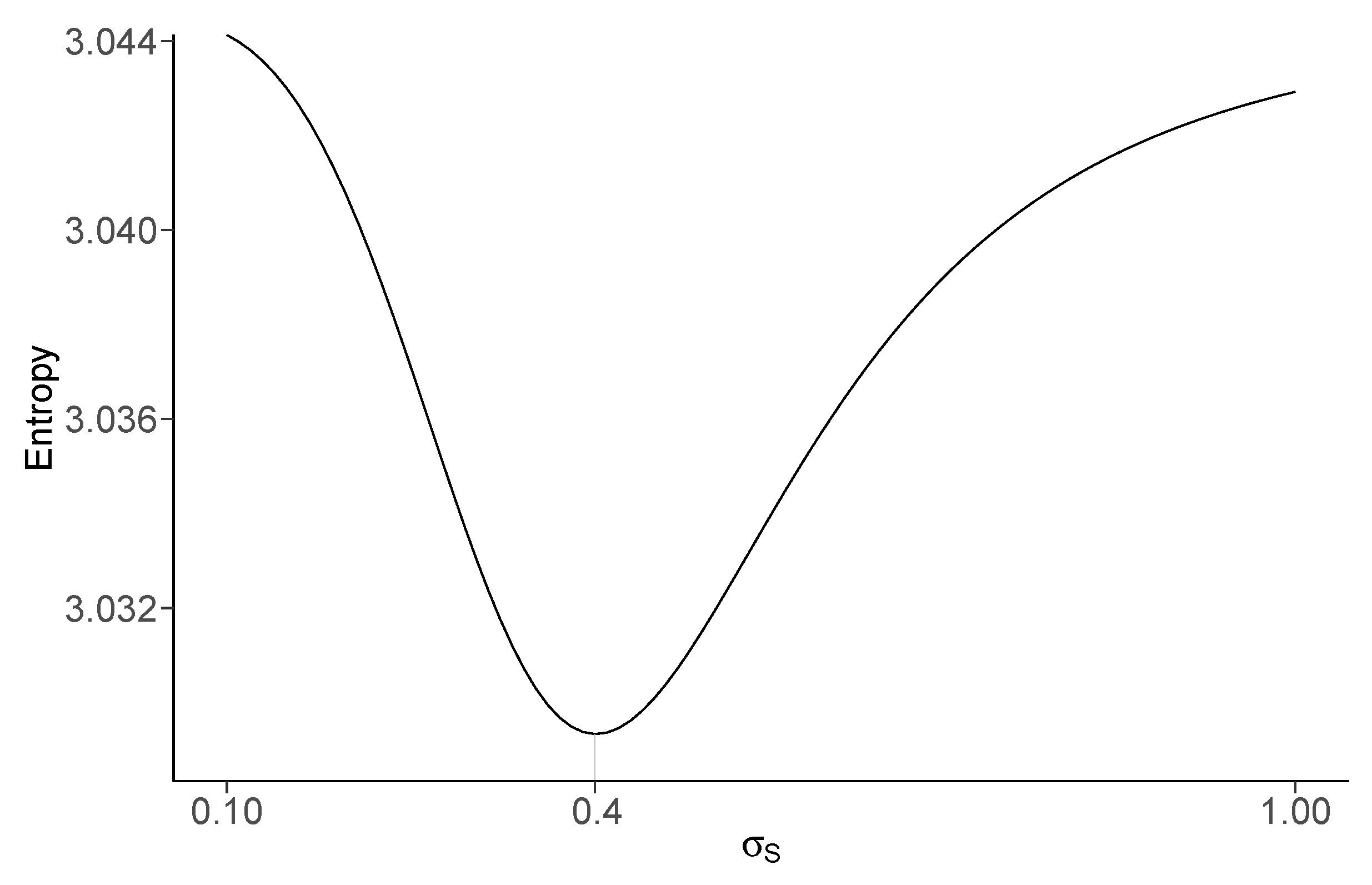
Figure 2 presents the entropy function of σ S computed from the data used for this study, which indicates that it is at its minimum at σ S = 0.4 . It is interesting to note that the entropy function increases as σ S decreases from 0.4 to zero. This is explained by looking into the similarity measure 1 + j i M e x p ( S i j σ S ) . As σ S moves toward zero, this measure converges at one for all i. Thus, s i moves toward one, and I i is close to 1 / M for all i. Because we want to have a shape parameter σ S that can differentiate the I-weights most distinctly with minimum uncertainty, the value σ S = 0.4 minimizing the entropy is chosen in this study.

4.4. Selection of σ D

To select an appropriate value of σ D for the P-weights, we attempted to use the entropy criteria again, but we were not fortunate enough to obtain the optimal result, as with σ S . Thus, a technique based on the p-value of the chi-square statistic [54] is considered in this study.
We denote P i ( σ D ) as a normalized P-weight for model i and for the given σ D , which is defined as follows:
P i ( σ D ) = e x p ( D i σ D ) l = 1 M e x p ( D l σ D ) ,
where D i is the performance measure of the i-th model.
For testing the hypothesis frame, the null hypothesis and the alternative hypothesis for i = 1 , , M are as follows:
H 0 :   all   weights   are   equal P i = 1 M   for   all   i H 1 :   some   weights   are   not   equal P i 1 M for   some   i .
For the given P i , the chi-square statistic used to test the above hypothesis is as follows:
χ 0 2 ( σ D ) = i = 1 M ( 1 M P i ( σ D ) ) 2 1 M .
Because we do not want to accept equal weights, σ D should be selected to reject the null hypothesis. That is, the p-value [54] obtained from the chi-square statistic should be less than a preassigned value α (significance level), e.g., α = 0.05 . In addition, because we also do not want aggressive weights, a σ D can be selected as the maximum value of σ D in which we still reject H 0 with α level. That is, our selection is
σ D = m a x { σ D : p - value ( σ D ) < α } ,
where p-value ( σ D ) = P r [ χ 2 > χ 0 2 ( σ D ) | H 0 ] .
Here, χ 2 indicates a random variable of (9) under the equal P i weights. Although this selection assures the use of the least aggressive weights, it is still statistically significantly different from the equal weights.
The p-values are computed by a Monte-Carlo simulation in which random numbers of weights are generated from the Dirichlet distribution [63]. When the parameters are all equal to 1, the Dirichlet distribution is the same as the multivariate uniform distribution with values between 0 and 1, which represents the null hypothesis. We used the “MCMCpack” package [64] in R to generate the random weights that satisfy H 0 .
The detailed steps of computing the p-value for given σ D and χ 0 2 ( σ D ) are:
  • Step 1: Generate random weights P i ( k ) from the Dirichlet distribution with all parameters equal to 1 (under H 0 ), for i = 1 , , M ;
  • Step 2: Compute χ 2 = i = 1 M ( 1 M P i ( k ) ) 2 1 / M , and denote it χ ( k ) 2 ;
  • Step 3: Iterate the above two steps K (=1000, for example) times;
  • Step 4: Calculate p - value ( σ D ) = k = 1 K I [ χ ( k ) 2 > χ 0 2 ( σ D ) ] K ,
where I [ A ] denotes the identity function, which takes 1 or 0, depending on if the condition A is satisfied or not. Note that P i ( k ) s generated in Step 1 do not depend on σ D .
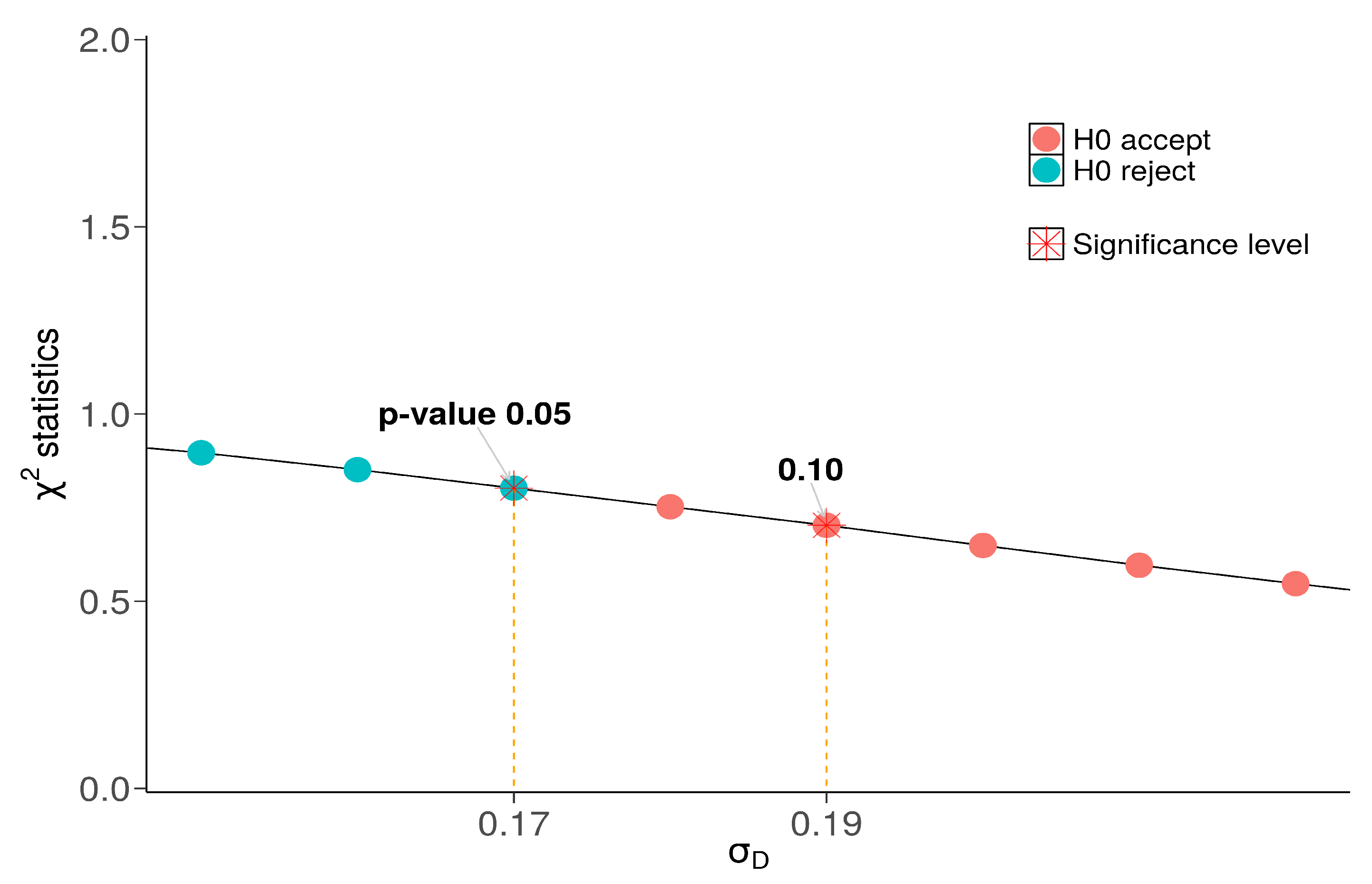
Figure 3 depicts the chi-square statistic values computed from AMP1 with some p-values as σ D changes from 0.10 to 0.30 in increments of 0.01. We calculated the σ D for each of the five climate variables, and then calculated the average from those five σ D s. When α = 0.05 , as is usually applied in testing a hypothesis in statistics, the averaged σ D from five different σ D is 0.21. When α = 0.1 , σ D = 0.25 . We use σ D = 0.21 in this study.

5. Results: Model Weights

5.1. Model Similarity

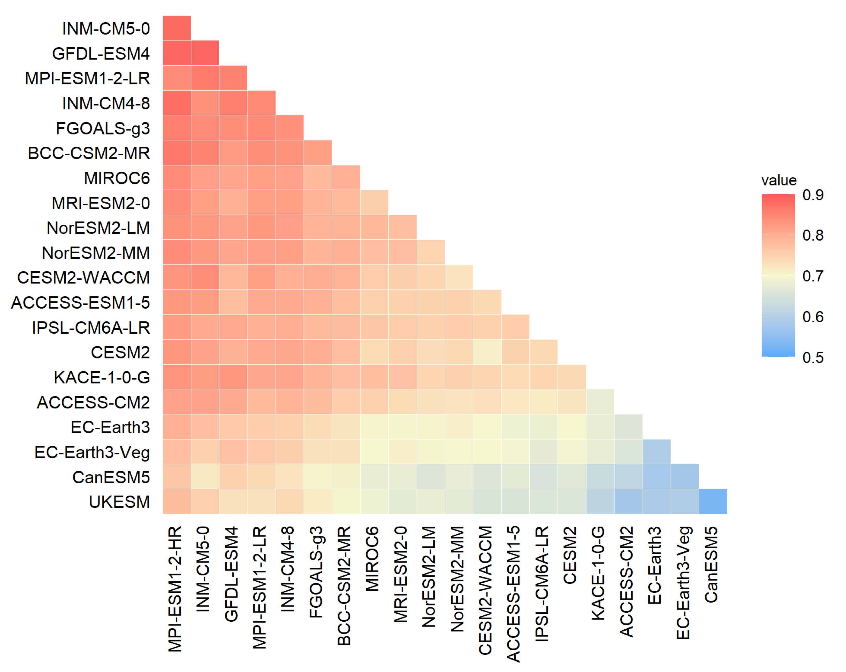
Table S2 provides the similarity values S i j for certain models. Figure 4 shows the intermodel distance matrix for the 21 CMIP6 models considered in this study. The distances are obtained from the five climate variables listed in Table 1 for East Asia. Each box represents a pairwise combination, where red indicates a greater distance. According to Figure 4, models MPI-ESM1-2-HR, INM-CM5-0, GFDL-ESM4, MPI-ESM1-2-LR, and INM-CM4-8 were found to be the most independent, whereas models UKESM, CanESM5, EC-Earth3-Veg, and EC-Earth3 were found to be the most dependent.

5.2. PI-Weights

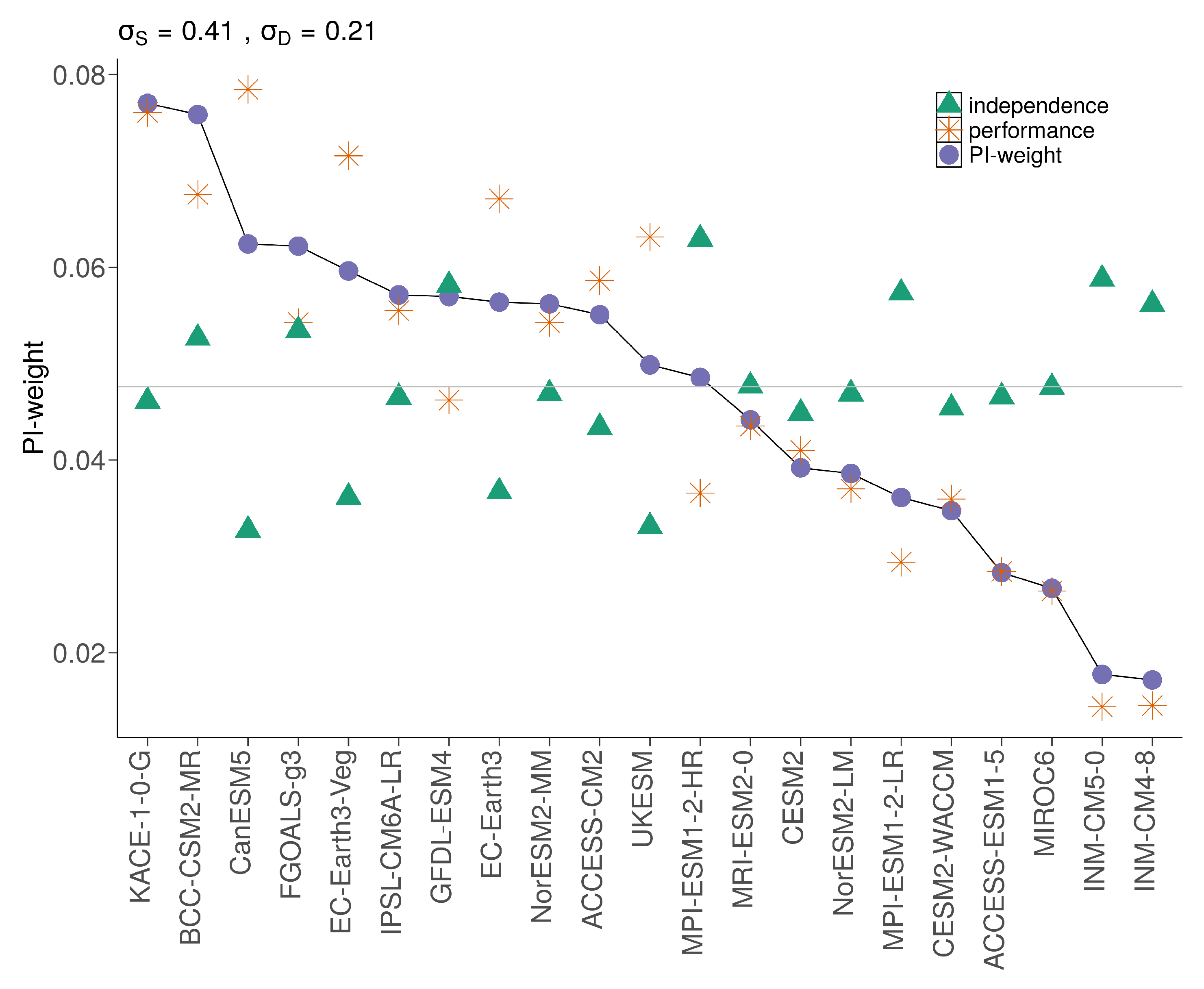
The normalized PI-weights are obtained using Equation (2) with σ S = 0.4 and σ D = 0.21 . Figure 5 demonstrates the distributions of the P-, I-, and PI-weights. The variability of the I-weights is smaller than that of the P-weights.
The high P-weights of the CanESM5 and EC-Earth3-Veg models decrease in the PI-weights owing to the low I-weights. The PI-weights of the BCC-CSM2-MR, FGOALS-g3, and GFDL-ESM4 models increase owing to a relatively high independency. The PI-weight is not located in the middle of the P- and I-weights, but is close to the P-weight, except in a few cases. When the P-weight (I-weight) is almost the same as the equal weight, as in the GFDL-ESM4 (KACE-1-0-G and IPSL-CM6A-LR) model, it seems that the PI-weight is wholly influenced by the I-weight (P-weight). The performances for some of the models, such as ACCESS-ESM1-5, MIROC6, INM-CM5-0, and INM-CM4-8, are so low that their (even relatively high) I-weights do not affect the final weights. Based on this view, the performance is more influential to the PI-weights than the independency. Some of these observations may be changed if different σ S and σ D are used.

6. Results: Future Projection of Extreme Precipitation

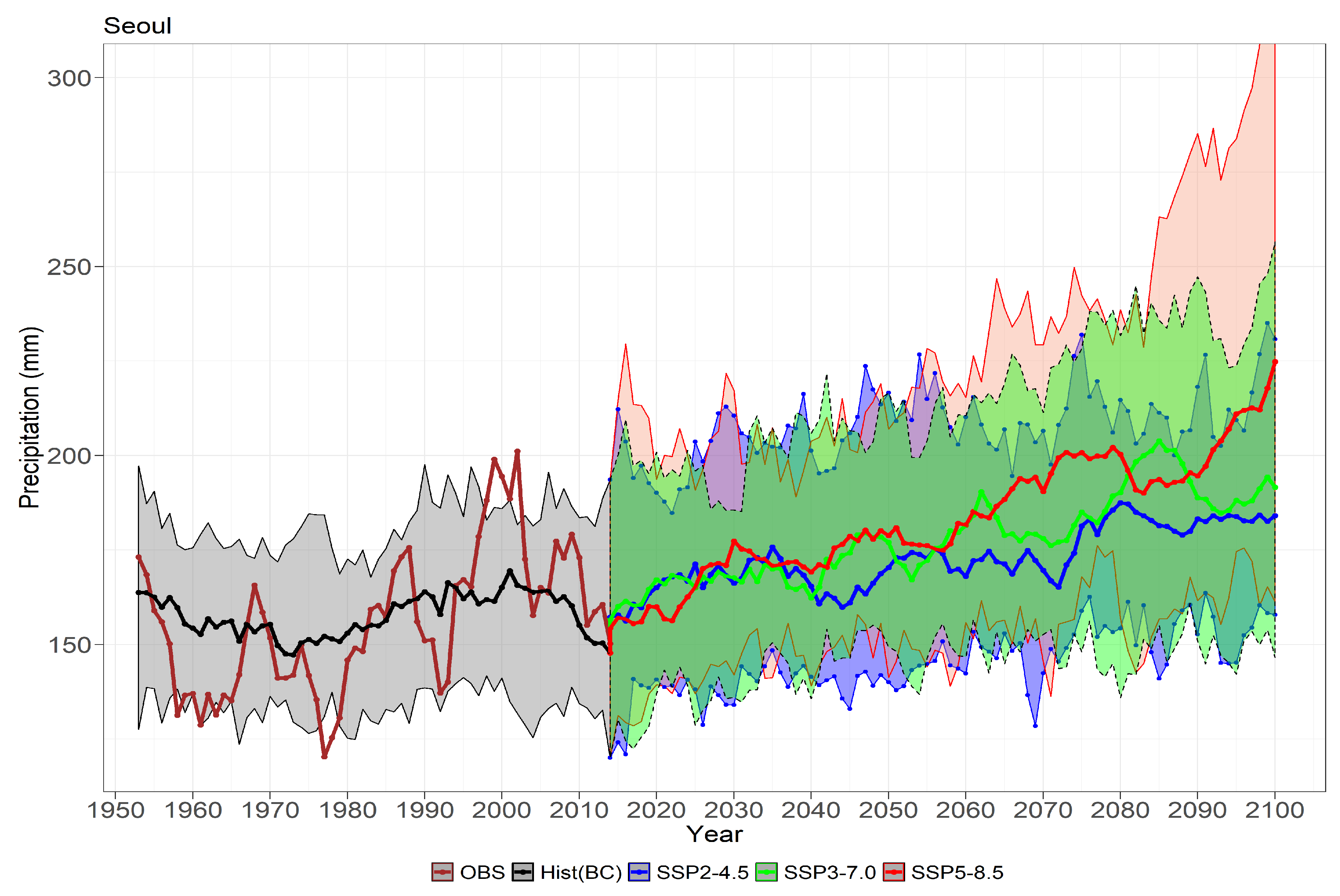
Using the PI-weights obtained in the above section, the future extreme precipitations are projected by the MME. Note that the future climate data are used after the bias correction with the MBC method [59]. Figure 6 illustrates the time series plots of the nine-year moving averages of AMP1 in Seoul, for example, from the observations, from the PI-weighted ensemble of the historical data, and from the PI-weighted ensembles for the future data from the three SSP scenarios, with a 90% confidence band. In Figure 6, the line for the observations shows more variation than the lines of the historical data and the future projections by the MME. This means that the MME has smaller variance and can catch the signal more clearly than a single simulation model.

6.1. Return Levels

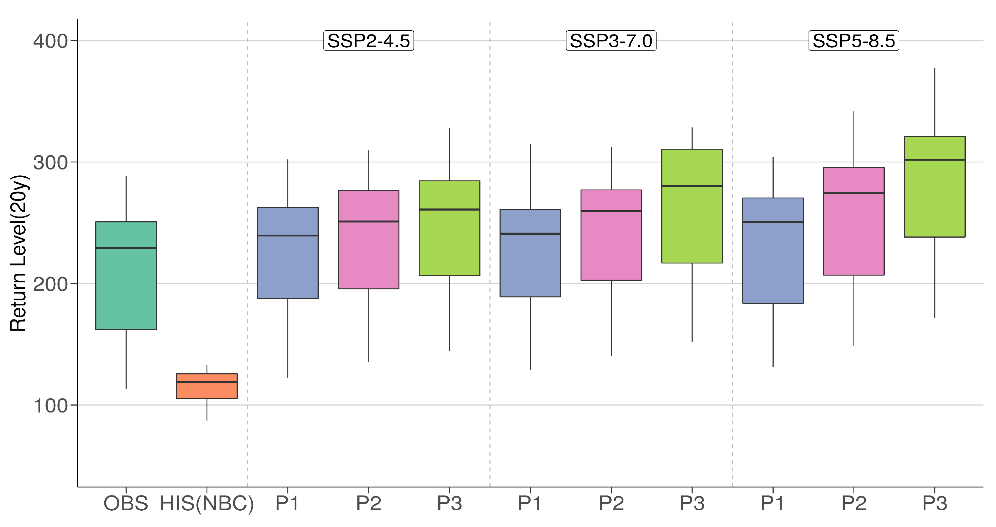
Figure 7 (S3) displays boxplots of the 20-year (50-year) return levels of the AMP1 in the KP. The boxplot of the historical data after the BC is similar to that from the observations, whereas the boxplot before the BC is much smaller than that from the observations. The increasing trends from P1 to P3 are evident in every scenario. Summary statistics of the corresponding values of these boxplots are provided in Table S3.
These values are lower in the 20-year return levels than the results by Lee et al. [27], who used the BMA method with the CMIP5 models. The median values for P3 in Table S3 are higher than the results by Shin et al. [41], who used the CMIP6 models and a hybrid weighting method between the BMA and equal weighting. It seems that the hybrid weighting by Shin et al. [41] and the PI-weighting in this study are similar. These last two weighting schemes assigned relatively lower weights to the CMIP6 models with heavy future precipitation than a weighting method based on the performance only would give to the same models.
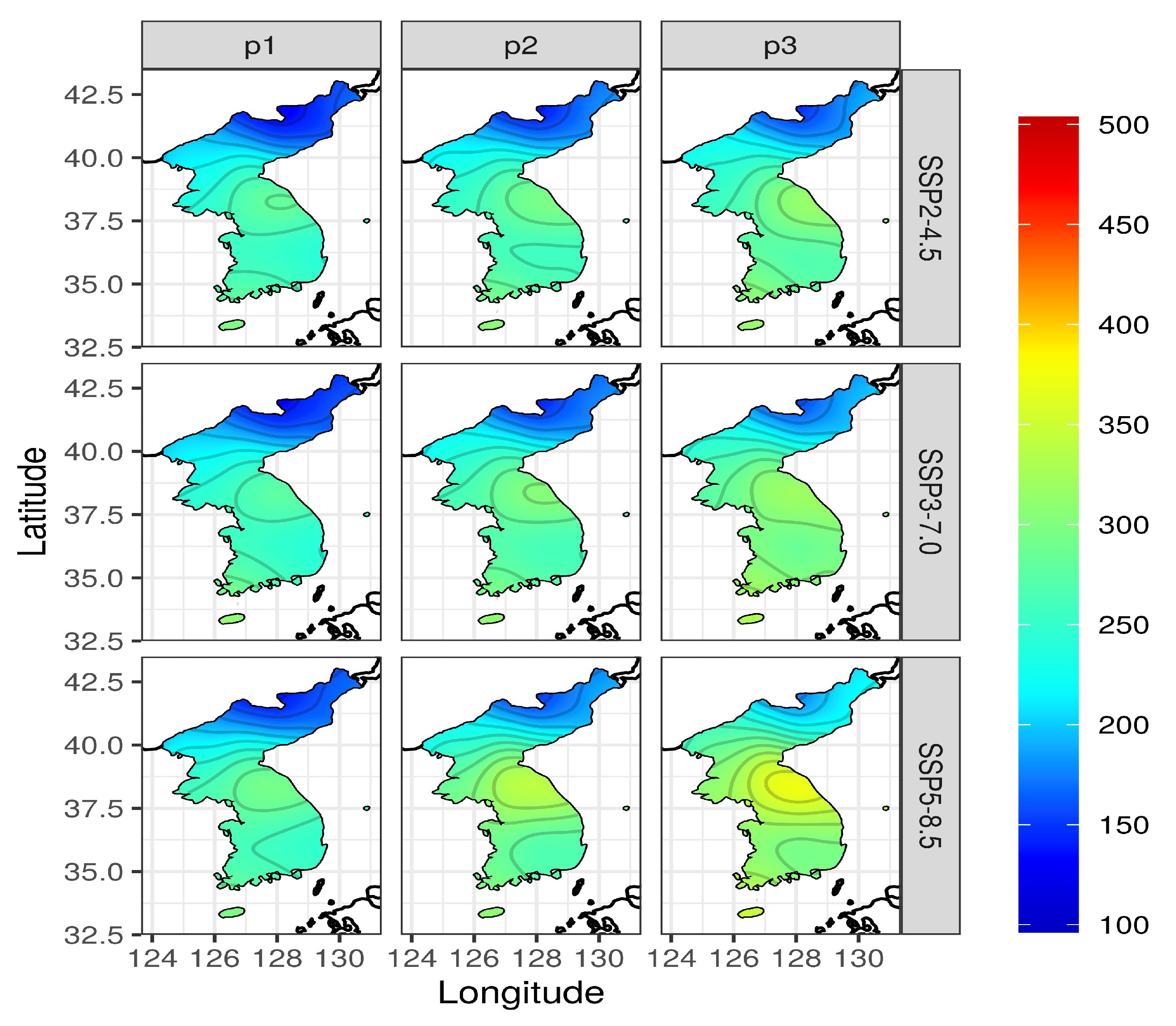
Figure 8 (S4) shows isopluvial maps of the 20-year (50-year) return levels of the AMP1 for the three future periods under the three scenarios. The difference by latitude is more evident than that by longitude. Jeju island, the southern coast, and the central region receive more downpours than the northern parts.

6.2. Changes in Return Levels

Figure S5 in the Supplementary Materials exhibits relative changes (unit: %) of the 20- and 50-year return levels of extreme precipitation over the Korean peninsula relative to the years 1973–2010. The increasing changes are more evident in the northern part than in the southern area. Summary statistics of relative changes are presented in Table S4 in the Supplementary Materials. The relative increase in the observations for the spatially averaged 20-year (50-year) return level was approximately 18.4% (18.9%) in the SSP2-4.5, 25.9% (26.3%) in the SSP3-7.0, and 41.7% (44.0%) in the SSP5-8.5 scenario by the end of the 21st century.
These rates of change are lower than the results by Lee et al. [27], who used the BMA method with the CMIP5 models. This is perhaps due to the differences in the reference period and the research methods, as well as the difference between the CMIP5 and CMIP6. For the 20-year return level, our result in the KP is approximately 1.8 to 2.0 times faster than the changes in the globally averaged value (10% in the SSP2-4.5 and 20% in the SSP5-8.5) reported by Kharin et al. [65].

6.3. Change in Return Periods

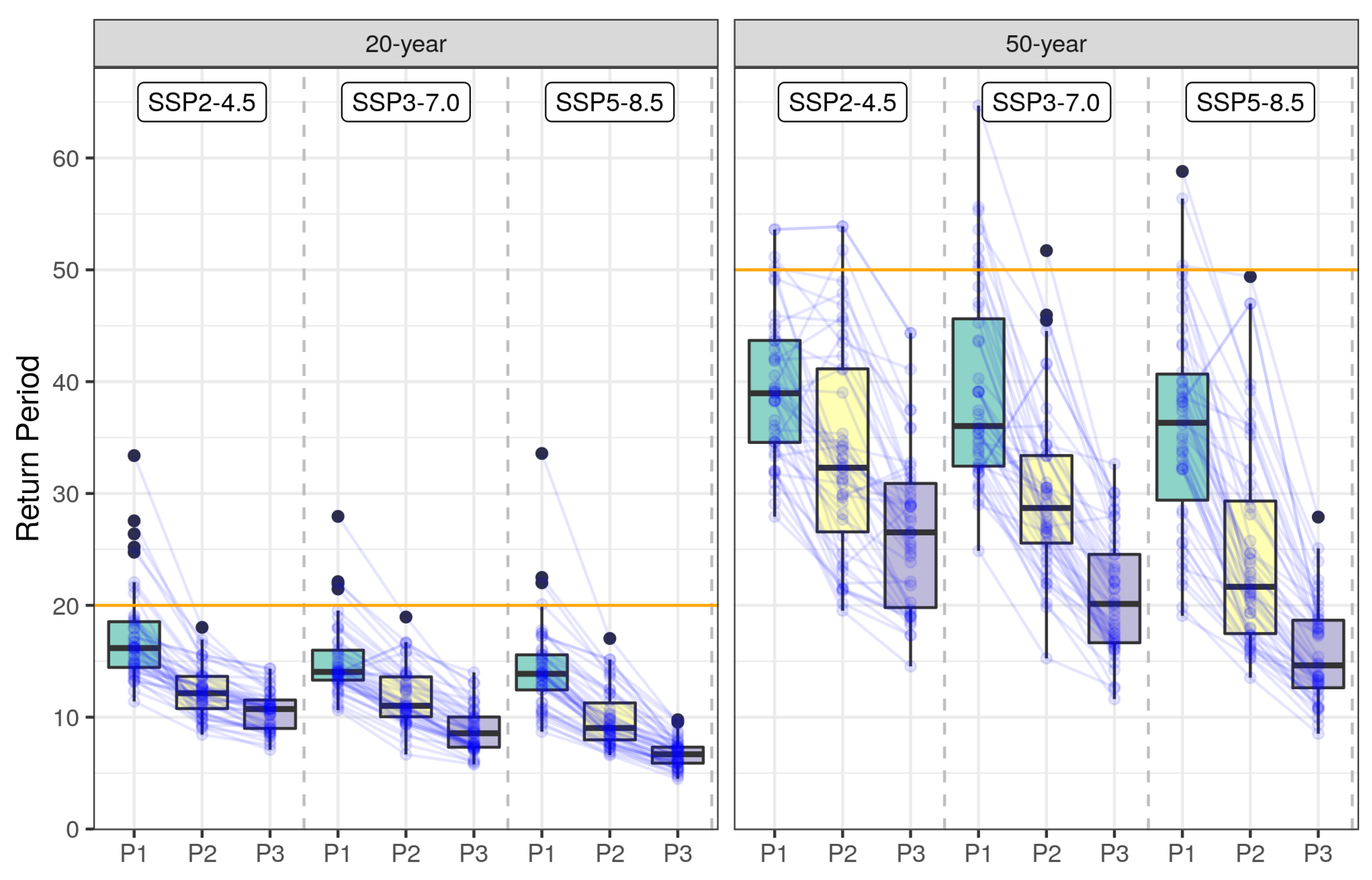
Figure 9 displays boxplots for the 20-year and 50-year return periods, as compared to the reference years (1973–2010) for the three future periods under the three scenarios. The corresponding statistics are presented in Table S5 in the Supplementary Materials. We realize that a 1-in-20 year (1-in-50 year) AMP1 in the Korean peninsula will likely become 1-in-11 (1-in-26) year, 1-in-8 (1-in-20) year, and 1-in-7 (1-in-15) year events in the median by the end of the 21st century based on the SSP2, SSP3, and SSP5 scenarios, respectively, as compared to the observations from 1973 to 2010. These findings indicate that both 20-year and 50-year return periods are likely to decrease by approximately 32% under the SSP2 and 60% under the SSP5 by the end of the 21st century.
These projections of extreme rainfall are similar to or less frequent than the results obtained by previous studies [23,27] based on CMIP5 models, i.e., approximately 1-in-11 (1-in-21) year and 1-in-7 (1-in-13) year events under SSP2 and SSP5, respectively. Shin et al. [41] realized the occurrence as approximately 1-in-10 (1-in-30) and 1-in-8 (1-in-17) year events under SSP2 and SSP5, respectively, which is similar to our projection.

6.4. Exceedance Probability and Waiting Time

Because of computational issues and the defects of the return period [66], the exceedance probability is often used as an alternative to the return period [67]. This is defined as P r [ Y ( θ ^ ) > z ] , where z is a specified precipitation value and Y ( θ ^ ) is a random variable following a GEVD with a parameter estimate θ ^ . Here, Y ( θ ^ ) depends on the models, periods, and scenarios.
The spatially averaged estimates of the exceedance probability are presented in Figure S6 and Table S6. There are relatively large differences in the exceedance probability of a downpour of 100 to 250 mm compared with that for over 250 mm, as shown in Figure S6. The differences between the past and future scenarios are distinct during the period P3.
From Table S6, the return period or expected waiting time ( T ( z ) ) until the reoccurrence of a specific AMP1 value (z) is computed by T ( z ) = 1 / p ( z ) , where p ( z ) is the exceedance probability of the AMP1 z. These values are listed in Table 2. For z = 200 mm of rainfall, for example, the expected waiting times until a reoccurrence are 11.1 years in the past, 13.0 years in the future period P1, 8.0 years in P2, and 5.9 years in P3 based on the SSP5 scenario. For the case of a z = 300 mm downpour, the expected waiting times are 78 years in the past, 76 years in P1, 50 years in P2, and 29 years in P3 based on the SSP5 scenario.

6.5. Expected Number of Reoccurring Years

Another quantity that we can obtain is the expected number of reoccurrences during a certain period. By multiplying 30 years by the exceedance probability p ( z ) , we can estimate the expected frequency of such years over a period of 30 years in which we have more than z amount of AMP1 for a year. These values are given in Table S7. For z = 150 mm (200 mm), as a specific example, during the last 30 years, we have experienced 6.8 (2.7) years in which AMP1 was greater than 150 mm (200 mm). In addition, we are likely to have an expected number of years of 8.2 (2.3) for the future period P1, 10.1 (3.8) for P2, and 12.1 (5.1) for P3 under the SSP5 scenario.
From this comparison, particularly for AMP1 of 100 to 300 mm, the expected number of years of occurrence for the future periods under the SSP5 scenario increases by approximately 1.25 times that over the last 30 years for P2 and 1.91 times that for P3 by the end of 21st century. These results are based on the spatially averaged values. When the exceedance probability is considered for each grid, different local results will be obtained.

7. Results: Projection by Latitude and Quantifying Uncertainty

Three or four major sources of climate projection uncertainty might be considered when trying to understand uncertainties in projected metrics: (1) climate model, (2) emission scenario, and (3) internal variation or randomness unexplained by other sources [68]. We apply the analysis of variance (ANOVA) technique [69] in this study. Other methods considered in [67] can also be applied.

7.1. Variance Decomposition with Interaction

Hawkins and Sutton [68] applied a method of variance decomposition to quantify uncertainty when assuming no interactions between the sources. In addition to their assumption, we added the interaction term between the model and scenario. Other factors, i.e., (4) future period and (5) location, such as the latitude applied in this study, are also considered in the ANOVA model. Although the period and latitude may not be real sources of uncertainty, they can be included as independent variables in the ANOVA model because they may affect the response variable. Here, the response variable is a 20-year return level, for example.
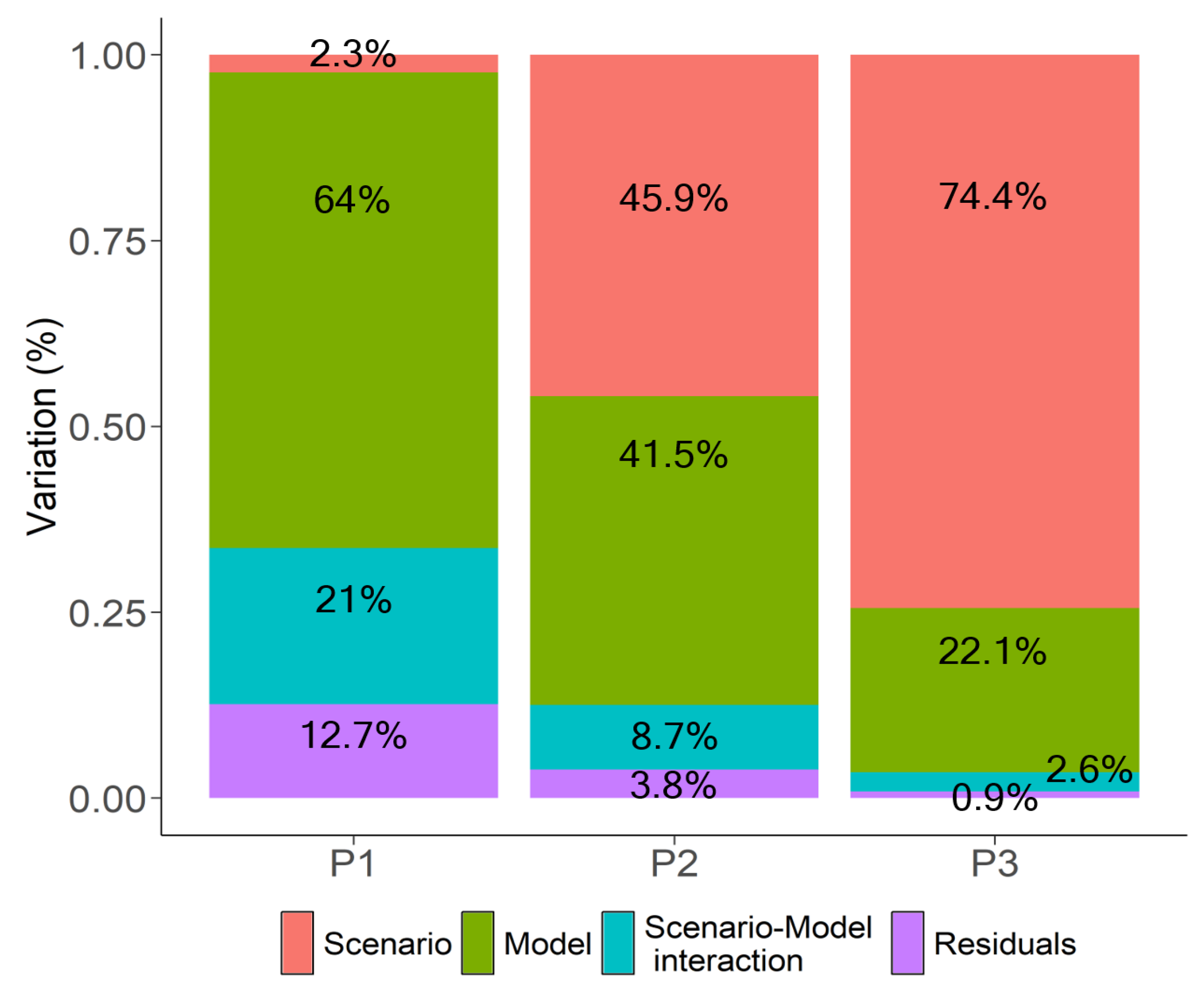
Figure 10 presents the proportions of variances contributed by each variable for each period. In P1, the variance by the model is the largest, whereas that by the scenario is the smallest. The proportion of internal variation (residual) decreases from P1 to P3. The variance proportion by model decreases from P1 to P3, whereas the variation due to the scenario increases significantly from P1 to P3.
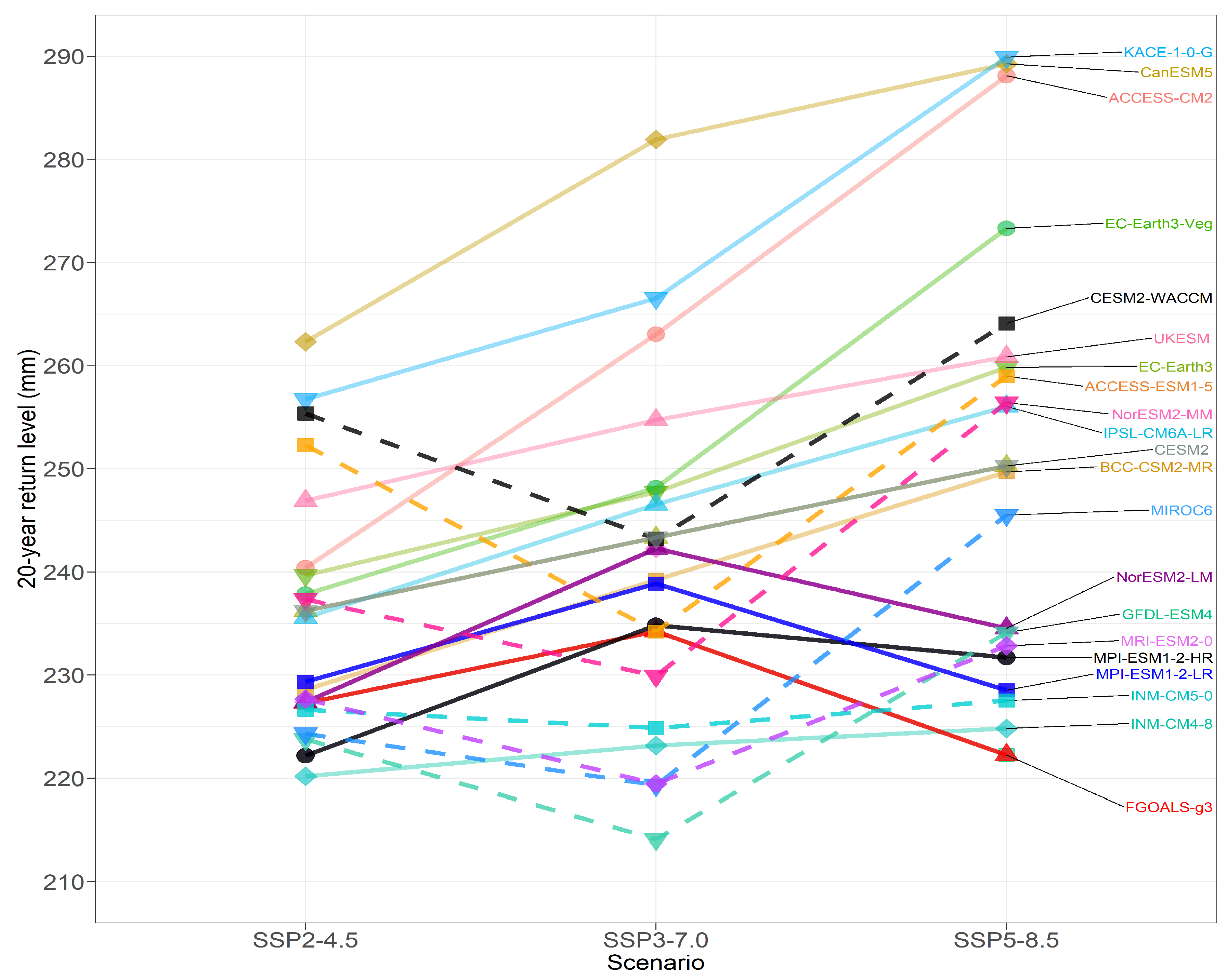
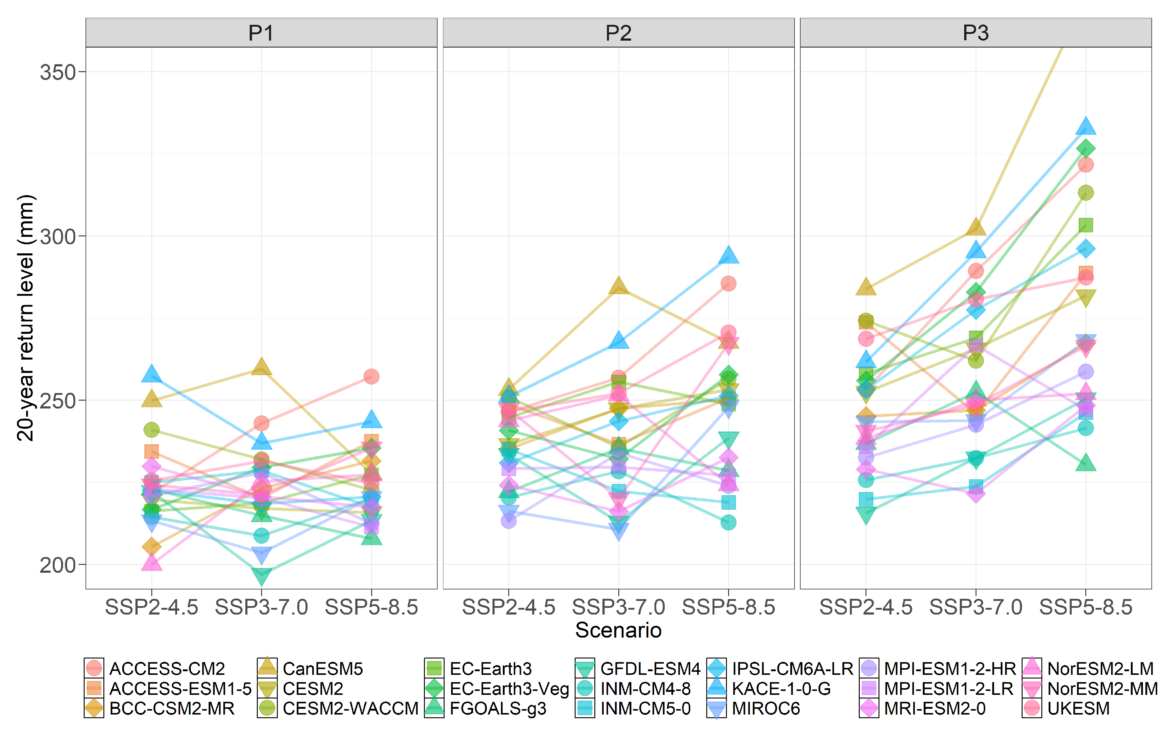
It is notable that the variation contributed by the interaction between the model and scenario is relatively large during period 1, but becomes smaller during period 3. The details of this variation are presented in Figure 11, where the return levels from the models generally increase in mean and variance as the scenario changes from SSP2 to SSP5. However, the return levels of some models, such as CESM2-WACCM, ACCESS-ESM1-5, NorESM2-MM, MIROC6, MRI-ESM2-0, GFDL-ESM4, and INM-CM5-0, decrease from SSP2 to SSP3, contrary to the expectation. Moreover, the return values of some models, such as MPI-ESM1-2-HR, MPI-ESM1-2-LR, NorESM2-LM, and FGOALS-g3, decrease from SSP3 to SSP5. The latter two “unexpected” situations make the interaction variance large in P1, as shown in Figure 12. Despite such “unexpected” situations still appearing in P3, the variations owing to the scenario and model themselves are relatively too large, and thus, the proportion of the interaction variance becomes relatively small in P3.

7.2. Return Levels by Latitude

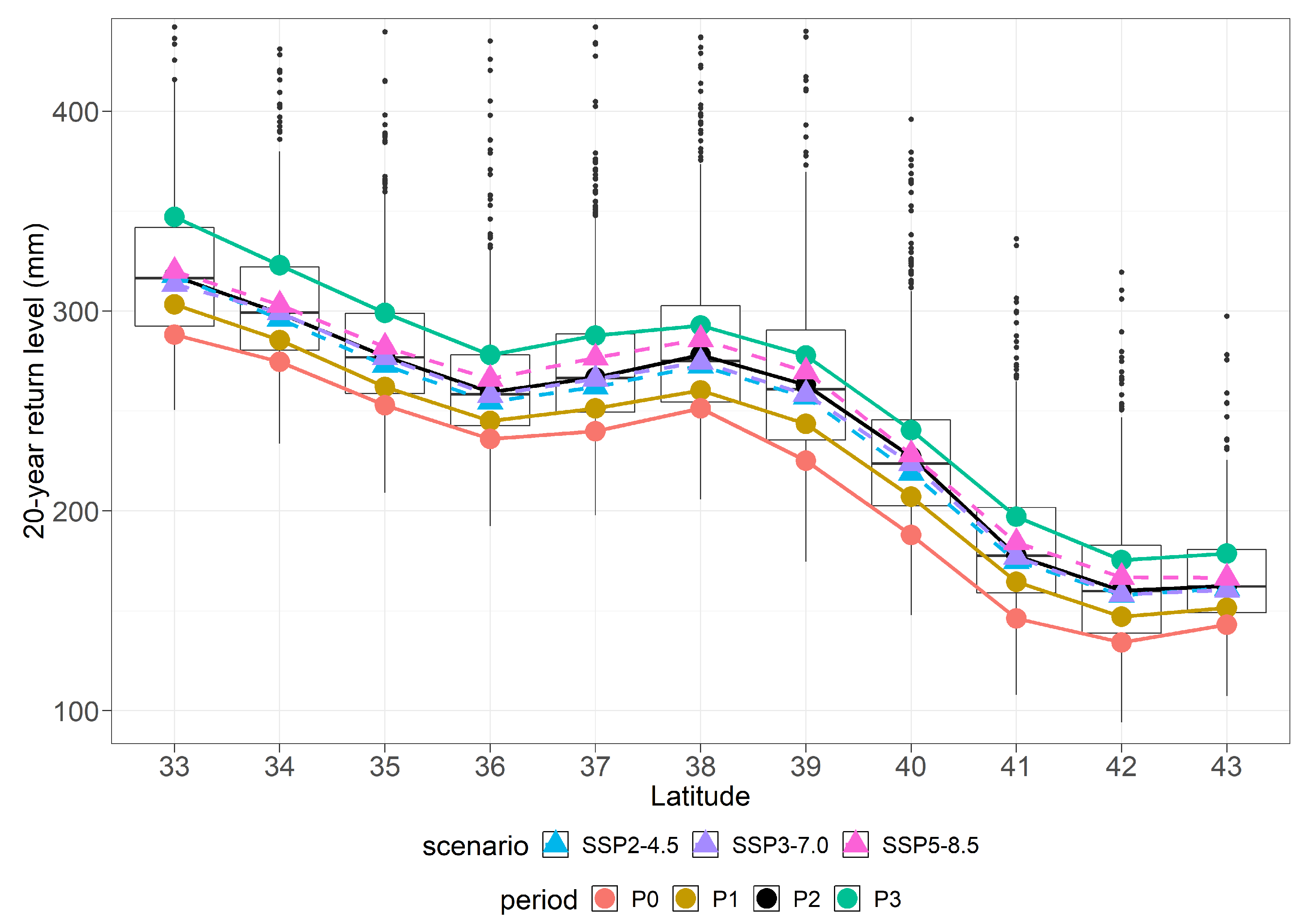
Figure 13 depicts boxplots of the 20-year return levels (unit: mm) from the 21 CMIP6 models as the latitude changes from south to north. It is evident that the return levels decrease initially from 33 to 36 , but increase from 36 to 38 . However, they decrease from 38 to 42 more rapidly. In Figure 13, the solid lines around the boxes across the latitude are the spatial medians of the 20-year return levels for each latitude and the four periods (P0, P1, P2, and P3). Here, P0 indicates the reference period, and thus, the result is obtained from the observations. The dashed lines depict the values for the three scenarios (SSP2-4.5, SSP3-7.0, and SSP5-8.5), in which three dashed lines locate the inside range of the solid lines. The spatial medians for the scenario (period) are obtained over all values across the periods (scenarios) for the 21 models. It is notable and interesting that the variation owing to the scenario is smaller than that from the period. Future projections fluctuate less than the observations.
The detailed values of the 20-year return levels of AMP1 and annual maximum five-day precipitation (AMP5) by latitude are presented in Table 3. These localized values provide different information from the previous results based on the spatial medians and averages over the Korean peninsula (Table S3). Table 3 indicates that a much higher intensity occurs in the southern part of the Korean peninsula than in the northern part. When the areas below and above 38 are considered the south and north, respectively, the south is likely to receive approximately 1.54 (1.72) times heavier rainfall in the 20-year return levels of AMP1 on average than the north (the spatial median) based on a rough calculation using the above tables. Although we did not obtain these values, the localized values of the return periods, the relative changes in the return levels, the exceedance probabilities, and the expected number of occurring years can be obtained for each latitude. Those values in the south would show higher intensity during extreme precipitation with shortened expected waiting times compared to the spatial medians throughout the Korean peninsula.

8. Comparison of PI-Weighted Ensembles to the Simple Average

For comparison between the PI-weighting scheme and the simple average for the multimodel ensemble, we consider two measures. The first one is the error index I 2 based on Baker and Taylor [70] for the reference (historical) period. The second is the weighted variance of return level prediction [71,72] for the future periods. In computing these measures, non-bias-corrected data were used.

8.1. Error Index for the Historical Period

The error index can measure combined errors, that is, over multiple variables, compared to the observed climate [40]. However, we only evaluate our target variable AMP1 over the reference period 1973–2010. In a first step, the normalized error is calculated for the T-year return level as the difference between the PI-weighted multimodel and the observations:
e w 2 = n = 1 N ( S n o n ) 2 σ n 2 ,
where S n is the weighted multimodel T-year return level per grid point n. S n is calculated from the historical data that are not bias corrected. o n is the T-year return level obtained from the observations, and σ n is the standard deviation of o n . The corresponding e e q 2 is calculated for the nonweighted multimodel T-year return level. Note that, for each n, o n and σ n are unchanged between e w 2 and e e q 2 because those are computed from the observations on grid point n. Then, the error index is obtained by:
I 2 = e w 2 e e q 2 .
This index can be useful to evaluate if the weighted mean is improved compared to the simple average [40]. The smaller the I 2 , the larger the improvement in the weighted average compared to the simple average for the target variable (AMP1) for the reference period.
The computed values of I 2 in this study are 0.622 for PI-weights and 0.627 for P-weights for the 20-year return level. Thus, there are 37.8% and 37.3% improvements in the PI-weighted and the P-weighted averages, respectively, compared to the nonweighted average. The decrease of the error index by adding I-weights from P-weights is 0.005, which is a 0.80% decrease relative to that of the P-weights. The results for the 50-year return level are similar to these.

8.2. Prediction Variance for the Future

The second measure to compare is from the weighted variance formula [71,72]:
V a r ( r ( T ) ) = k = 1 K [ r k ( T ) r ¯ ( T ) ] 2 w k + k = 1 K V a r ( r k ( T ) ) w k ,
where r ( T ) is the T-year return level, r k ( T ) is the T-year return level from the k-th model, and r ¯ ( T ) = 1 K k = 1 K r k ( T ) w k . The first term of (13) is the among-model variance, and the second one is within-model variance. V a r ( r k ( T ) ) is estimated using a bootstrap technique in this study. Based on this variance, we quantify the skill of the PI-weighted method with the Brier skill score [54]:
B S S = 100 × { 1 V a r P I V a r E q } ,
where V a r P I is the variance of the T-year return level calculated by (13) from the PI-weights, and V a r E q is the variance calculated by (13) from the equal weights for each grid point. BSS is a relative quantity and shows a percentage improvement of the PI-weighted method over the simple average.
Figure 14 shows the differences of variances of 20-year return levels calculated from the PI-weights and the equal weights plotted for 46 grid points for each future period and for each scenario. V a r P I for the Y-axes is the variance calculated by Equation (13) from the PI-weights. V a r E q for the X-axes is the corresponding variance calculated from the equal weights. In the top panel, more points are located below the diagonal lines, which means that the variances calculated from the PI-weights are smaller more often than those from the simple average. The middle (bottom) panel shows the differences of between-model (within-model) variances. V a r B M , P I and V a r W M , P I for the Y-axis are between-model and within-model variances from the PI-weights, respectively, and V a r B M , E q and V a r W M , E q for the X-axis are the corresponding variances calculated from the equal weights. The within-model variances from both weights are similar, as seen in the bottom panel. Thus, we know that the differences in total variances in the top panel are mainly because of the differences of between-model variances.
Table 4 reads the averaged values of BSS over 46 grid points, the averaged differences of variances (unit: mm 2 ) of the 20-year return level, and relative improvements (RIs) for three periods and for three scenarios. The BSS values range from −2.2% to 22.5%. The averages of BSS over all periods are 6.29% for SSP2, 15.2% for SSP3, and 13.1% for SSP5 (11.5% overall). These averages of BSS also increase as the period moves from P1 to P3. The BSS due to between-model variance is bigger than that due to within-model variance. Watching the sixth to the eighth columns of this table, we know that the positive differences of two variances ( V a r E q V a r P I ) are mainly because of the differences of two between-model variances ( V a r B M , P I V a r B M , E q ). These patterns are prominent for the SSP5-8.5 scenario with increasing values from P1 to P3. The last column shows the RI of the PI-weighted method over the simple average in the variances. The RI values range from −3.3% to 26.0%. The averages of RI over all periods are 7.45% for SSP2, 19.1% for SSP3, and 14.0% for SSP5 (13.5% overall). These averages of RI also increase as the period moves from P1 to P3.

9. Discussion

It is generally accepted that increasing greenhouse gases induce atmospheric temperature warming, which results in increasing equivalent potential temperatures and specific humidity, according to the Clausius–Clapeyron relationship [73]. The increase in atmospheric water vapor is the main factor in generating convective instability. In view of this insight, Kim et al. [26] obtained an indication that increasing the extreme precipitation over South Korea in the past and future scenarios is related more to a change in convective instability rather than to synoptic conditions. Another plausible explanation for the increase in the maximum precipitation over the Korean peninsula is the increase in both the frequency and strength of typhoons in the region. Typhoons have a greater influence on the southern area than the northern part. The occurrence of extreme rainfall in the southern part is related to more sources or variables than in the northern area [25,26].
We observed a scale discrepancy between the model grids and the observation stations, which may compromise the credibility of our results. Regional projections require a fine resolution of the simulation models, whereas some of the CMIP6 models have a coarse resolution. It is known that the model spread is one of the major sources of uncertainty in regional predictions (Hawkins and Sutton, 2009). However, large numbers of simulation models can reduce the uncertainty and provide a robust projection [74,75]. A total of twenty-one CMIP6 models with different scales used in this study can cover the study region with a finer spatial structure to increase the reliability of the projection.
The daily precipitation data consist of measurements from 00:00 to 24:00 throughout the day. In daily observations, the rainfall does not accumulate between 22:00 and 02:00. In the data used in this study, such precipitation is divided and recorded in two separate days. The actual serious daily risk due to heavy rainfall does not exactly depend on the precipitation over the time duration from 00:00 to 24:00 exclusively. It is therefore recommended to consider the AMP1 data based on the maximum precipitation during the 24 h movement. In this sense, the results presented in this study underestimate the actual intensity and frequency of AMP1. More realistic daily data, such those as obtained after moving for 24 h and the annual maximum of two (and several) days of precipitation, should be used in a future study for assessment of risk owing to extreme rainfall.
Brunner et al. [36,61] considered multiple observational (or reanalysis) datasets to include an estimate of the observational uncertainty. They proposed a novel approach to account for the observational spread and uncertainty in a multi-model weighting study, which can lead to robust results and a more precise uncertainty quantification. In addition, considering multiple observational datasets may address the problem in which the BC and performance-based weighting scheme utilize an excessive number of observations. We believe that using the observations twice in the BC and weight calculation is unadvisable. Xu et al. [35] considered a Bayesian weighting method that removes observations during the initial phase of the downscaling and adds them in the estimation of the posterior distribution. However, if the series of observations is sufficiently long to divide into two parts, we may use one part for the BC and the other part for the weight calculation. Although we did not apply these methods, this would be a good approach in a future study.
In determining the shape parameter σ D for the performance weights, we used the standardized return levels. However, as a different approach, the BMA method described in [27,41,72] can be employed. The BMA weighting does not need to standardize the return levels or determine the shape parameter σ D . It requires a bootstrap to estimate the variances of the return levels, which is straightforward in current computing facilities. Thus, calculating the P-weights based on the BMA, with an effort to minimize the probability of overconfidence, is recommendable.

10. Summary

We estimated the future changes in precipitation extremes within the Korean peninsula using observations, 21 multiple CMIP6 models, generalized extreme value distribution, the multivariate bias correction technique, and the model weighting method (PI-weighting), which account for both the performance and independence of the models. To avoid overfitting in the PI-weighting, we considered five climate variables for East Asia.
In applying the PI-weighting method, we suggest two ways of selecting two shape parameters, based on the p-value of the chi-square statistic and entropy. The suggested methods are simple and intuitively appealing, although they may need more justification for use in other studies.
From the analysis described this study, we realized that a 1-in-20 year (1-in-50 year) annual maximum daily precipitation within the Korean peninsula will likely become a 1-in-11 (1-in-26) year, a 1-in-8 (1-in-20) year, and a 1-in-7 (1-in-15) year event in terms of the median by the end of the 21st century under the SSP2-4.5, SSP3-7.0, and SSP5-8.5 scenarios, respectively, as compared to the observations from 1973 through 2010. These results are similar to or less frequent than those obtained by previous studies [23,27,41], but still, they predict more frequent and intensified extreme precipitation events by the end of the 21st century as compared to 1973 through 2010.
The expected frequency of the reoccurring years, particularly for AMP1 from 100 to 300 mm under the SSP5 scenario, is projected to increase by approximately 1.0 times that of the past 30 years for period 1 (2021–2050), approximately 1.25 times that for period 2 (2046–2075), and approximately 1.91 times that for period 3 (2071–2100).
From the analysis based on latitude, we found that extreme rainfall is more prominent in the southern and central parts of the peninsula. The downpour in the southern part is approximately 1.54 times heavier than that of the northern part and approximately 1.72 times that of the spatial median of the Korean peninsula. For example, for 150 mm of AMP1, the expected waiting times until reoccurrence in the southern part (spatial median of the peninsula) are 2.6 (4.4) years during the reference period, 2.1 (3.6) years during P1, 1.7 (3.0) years during P2, and 1.5 (2.5) years during P3 based on the SSP5-8.5 scenario.
Heavy rainfall can have a significant effect on human life, communities, infrastructure, agriculture and livestock, and natural ecosystems. Thus, in addressing the impact of climate change due to more frequent extreme precipitation events, governments and communities should prepare the proper infrastructure and systems more carefully and securely to prevent critical damage, such as loss of life from landslides and flooding.

Supplementary Materials

The following are available at https://www.mdpi.com/2073-4433/12/1/97/s1. Table S1: The list of 21 CMIP6 (Coupled Model Intercomparison Project Phase 6) models analyzed in this study. Table S2: The similarity distance metric S i j between model i and model j. Table S3: Statistics of 20-year and 50-year return levels of the annual maximum daily precipitation (unit: mm) averaged over 46 grids in the Korean peninsula for the observations (OBS) and the future periods under the three SSP scenarios. Table S4: Relative change (unit: %) in 20-year and 50-year return levels of the annual maximum daily precipitation averaged over the Korean peninsula relative to 1973–2010. Table S5: Statistics of 20-year and 50-year return periods (unit: year) of the annual maximum daily precipitation averaged over 46 grids in the Korean peninsula. Table S6: Spatially averaged the exceedance probability over the Korean peninsula for the annual maximum daily precipitation (AMP1) from 100   mm to 500   mm , obtained from the observations (OBS) and the CMIP6 models. Table S7: The expected frequency of reoccurring years during 30 years for specific the annual maximum daily precipitation (AMP1) values from 100   mm to 500   mm in the Korean peninsula, obtained from the observations (OBS) and the CMIP6 models. Figure S1: Examples of time series plots of the observations (black line), APHRODITE data (red line), and the bias-corrected data (blue line) in the Korean peninsula. Figure S2: Arrangement of data and 7-year moving averages composed of the historical data from 1850 to 2010 and the future data for computing the Spearman correlation coefficient between models. Figure S3: Schematic box-plots of 50-year return levels of the annual maximum daily precipitation (unit: mm) averaged over 46 grids in the Korean peninsula for the future periods under the three SSP scenarios. Figure S4: Isopluvial maps of 50-year return levels of the annual maximum daily precipitation for 46 grids over the Korean peninsula. Figure S5: Isopluvial maps of for the relative changes (unit: %) of 20-year and 50 return levels relative to 1973–2010 for the annual maximum daily precipitation for 46 grids over the Korean peninsula. Figure S6: The exceedance probability plots for the annual maximum daily precipitation (AMP1) from 50   mm to 300   mm in the Korean peninsula, obtained from the observations (OBS) and the CMIP6 models. Figure S7: Interaction plots between 21 CMIP6 models and the latitude in which the latitude changes from 33° to 43°, for 20-year return levels (unit: mm) computed over the Korean peninsula.

Author Contributions

Conceptualization, Y.S. (Yonggwan Shin), M.-K.K., and J.-S.P.; methodology, M.-K.K. and J.-S.P.; software, Y.S. (Yonggwan Shin), Y.S. (Yire Shin), and J.H.; validation, Y.-H.B., K.-O.B., I.-U.C., and D.-S.R.P.; investigation, I.-U.C. and D.-S.R.P.; data curation, Y.-H.B. and K.-O.B.; writing—original draft preparation, Y.S. (Yonggwan Shin), Y.S. (Yire Shin), and J.-S.P.; writing—review and editing, Y.-H.B. and J.-S.P.; visualization, Y.S. (Yonggwan Shin), Y.S. (Yire Shin), and J.H.; supervision, Y.-H.B., K.-O.B., and M.-K.K.; project administration, Y.-H.B., K.-O.B., and M.-K.K.; funding acquisition, M.-K.K., I.-U.C., D.-S.R.P., and J.-S.P. All authors have read and agreed to the published version of the manuscript.

Funding

This study was supported by a National Research Foundation of Korea (NRF) grant funded by the Korean government (MSIT) (No.2020R1I1A3069260) and BK21 FOUR funded by the Ministry of Education, Korea (I20SS7609010). The work of the NIMS authors was performed under the auspices of the Korea Meteorological Administration Research and Development Program “Development and Assessment of IPCC AR6 Climate Change Scenarios (KMA2018-00321)”.

Data Availability Statement

The CMIP data are available through ESGF’s website at https://esgf-node.llnl.gov/projects/ and DKRZ’s website at https://cera-www.dkrz.de/WDCC/ui/cerasearch/. Observational station data in the Korean peninsula are provided by KMA at http://data.kma.go.kr/. The APHRODITE data are available at http://aphrodite.st.hirosaki-u.ac.jp/download/.

Acknowledgments

The authors would like to thank the reviewers and the guest editors of the special issue for their helpful comments and suggestions, which have significantly improved the presentation of this paper. We acknowledge the World Climate Research Program Working Group on Coupled Modeling, which is responsible for CMIP, and we thank the climate modeling groups for producing and making available their model outputs. For CMIP, the U.S. Department of Energy Program for Climate Model Diagnosis and Intercomparison provided coordinating support and led the development of the software infrastructure in partnership with the Global Organization for Earth System Science Portals. We thank all contributors to the numerical R packages, which were crucial for this work. The authors are grateful to Seung-Ki Min (Division of Environmental Sciences and Engineering, POSTECH), who provided valuable comments to improve this paper.

Conflicts of Interest

The authors declare that they have no conflict of interest.

References

  1. IPCC. Managing the Risks of Extreme Events and Disasters to Advance Climate Change Adaptation. Special Report of the Intergovernmental Panel on Climate Change; Cambridge University Press: Cambridge, UK, 2012; Available online: http://ipcc-wg2.gov/SREX/report/ (accessed on 15 July 2020).
  2. Easterling, D.R.; Kunkel, K.E.; Arnold, J.R.; Knutson, T.; LeGrande, A.N.; Leung, L.R.; Vose, R.S.; Waliser, D.E.; Wehner, M.F. Precipitation Change in the United States. In Climate Science Special Report: Fourth National Climate Assessment; Wuebbles, D.J., Fahey, D.W., Hibbard, K.A., Dokken, D.J., Stewart, B.C., Maycock, T.K., Eds.; U.S. Global Change Research Program: Washington, DC, USA, 2017; Volume I, pp. 207–230. [Google Scholar] [CrossRef]
  3. Westra, S.; Alexander, L.V.; Zwiers, F.W. Global increasing trends in annual maximum daily precipitation. J. Clim. 2013, 26, 3904–3918. [Google Scholar] [CrossRef] [Green Version]
  4. Freychet, N.; Hsu, H.; Chou, C.; Wu, C. Asian summer monsoon in CMIP5 projections: A link between the change in extreme precipitation and monsoon dynamics. J. Clim. 2015. [Google Scholar] [CrossRef]
  5. Alexander, L.V. Global observed long-term changes in temperature and precipitation extremes: A review of progress and limitations in IPCC assessments and beyond. Weather. Clim. Extrem. 2016, 11, 4–16. [Google Scholar] [CrossRef] [Green Version]
  6. Park, C.; Min, S.K.; Lee, D.; Cha, D.H.; Suh, M.S.; Kang, H.K.; Hong, S.Y.; Lee, D.K.; Baek, H.J.; Boo, K.O.; et al. Evaluation of multiple regional climate models for summer climate extremes over East Asia. Clim. Dynam. 2016, 46, 2469–2486. [Google Scholar] [CrossRef]
  7. Dike, V.N.; Lin, Z.-H.; Ibe, C.C. Intensification of Summer Rainfall Extremes over Nigeria during Recent Decades. Atmosphere 2020, 11, 1084. [Google Scholar] [CrossRef]
  8. Lenderink, G.; van Meijgaard, E. Increase in hourly precipitation extremes beyond expectations from temperature changes. Nat. Geosci. 2008, 1, 511–514. [Google Scholar] [CrossRef]
  9. Berg, P.; Moseley, C.; Haerter, J.O. Strong increase in convective precipitation in response to higher temperatures. Nat. Geosci. 2013, 6, 181–185. [Google Scholar] [CrossRef]
  10. Scott, M. Prepare for More Downpours: Heavy Rain Has Increased across Most of the United States, and Is Likely to Increase Further. ClimateWatch Magazine; 2019. Available online: https://www.climate.gov/ (accessed on 25 July 2020).
  11. CISRO. Climate Change in Australia: Projections for Australia’s NRM Regions. Technical Report; 2015. Available online: https://www.climatechangeinaustralia.gov.au/media/ccia/2.1.6/cms_page_media/168/CCIA_2015_NRM_TechnicalReport_WEB.pdf (accessed on 15 May 2020).
  12. Mann, M.E.; Kump, L.R. Dire Predictions: Understanding Climate Change, 2nd ed.; DK Publishing: New York, NY, USA, 2015. [Google Scholar]
  13. Hov, Ø.; Cubasch, U.; Fischer, E.; Höppe, P.; Iversen, T.; Gunnar Kvamstø, N.; Kundzewicz, W.Z.; Rezacova, D.; Rios, D.; Duarte., S.F.; et al. Extreme Weather Events in Europe: Preparing for Climate Change Adaptation; Report produced by Norwegian Meteorological Institute in cooperation with EASAC; Norwegian Meteorological Institute: Oslo, Norway, 2013. [Google Scholar]
  14. Ho, C.-H.; Park, T.-W.; Jun, S.-Y.; Lee, M.-H.; Park, C.-E.; Kim, J.; Lee, S.-J.; Hong, Y.-D.; Song, C.-K.; Lee, J.-B. A projection of extreme climate events in the 21st century over East Asia using the community climate system model 3. Asia Pac. J. Atmos. Sci. 2011, 47, 329–344. [Google Scholar] [CrossRef]
  15. Kwon, S.H.; Kim, J.; Boo, K.O.; Shim, S.; Kim, Y.; Choi, J.; Byun, Y.H. Performance-based projection of the climate change effects on precipitation extremes in East Asia using two metrics. Intern. J. Climatol. 2019, 39, 2324–2335. [Google Scholar] [CrossRef]
  16. Mukherjee, S.; Aadhar, S.; Stone, D.; Mishra, V. Increase in extreme precipitation events under anthropogenic warming in India. Weather. Clim. Extrem. 2018, 20, 45–53. [Google Scholar] [CrossRef]
  17. Jung, H.S.; Choi, Y.E.; Lim, G.H. Recent trends in temperature and precipitation over South Korea. Int. J. Clim. 2002, 22, 1327–1337. [Google Scholar] [CrossRef]
  18. Choi, K.S.; Moon, J.Y.; Kim, D.W. The significant increase of summer rainfall occurring in Korea from 1998. Theor. Appl. Clim. 2010, 102, 275–286. [Google Scholar] [CrossRef]
  19. Park, J.-S.; Kang, H.-S.; Lee, Y.; Kim, M.-K. Changes in the extreme daily rainfall in South Korea. Intern. J. Clim. 2011, 31, 2290–2299. [Google Scholar] [CrossRef]
  20. Lee, Y.; Paek, J.; Park, J.S.; Boo, K.-O. Changes in temperature and rainfall extremes across East Asia in the CMIP5 ensemble. Theor. Appl. Clim. 2020, 141, 143–155. [Google Scholar] [CrossRef]
  21. Boo, K.O.; Kwon, W.T.; Baek, H.J. Change of extreme events of temperature and precipitation over Korea using regional projection of future climate change. Geophys. Res. Lett. 2006, 33, L01701. [Google Scholar] [CrossRef]
  22. Im, E.S.; Jung, I.W.; Bae, D.H. The temporal and spatial structures of recent and future trends in extreme indices over Korea from a regional climate projection. Int. J. Clim. 2011, 31, 72–86. [Google Scholar] [CrossRef]
  23. Seo, Y.A.; Lee, Y.; Park, J.-S.; Kim, M.-K.; Cho, C.; Baek, H.-J. Assessing changes in observed and future projected precipitation extremes in South Korea. Int. J. Clim. 2015, 35, 1069–1078. [Google Scholar] [CrossRef]
  24. Ahn, J.-B.; Jo, S.; Suh, M.-S.; Cha, D.-H.; Lee, D.-K.; Hong, S.Y.; Min, S.-K.; Park, S.-C.; Kang, H.-S.; Shim, K.-M. Changes of precipitation extremes over South Korea projected by the 5 RCMs under RCP scenarios. Asia Pac. J. Atmos. Sci. 2016, 52, 223–236. [Google Scholar] [CrossRef]
  25. Cha, D.-H.; Lee, D.-K.; Jin, C.-S.; Kim, G.; Choi, Y.; Suh, M.-S.; Ahn, J.-B.; Hong, S.-Y.; Min, S.-K.; Park, S.-C.; et al. Future changes in summer precipitation in regional climate simulations over the Korean Peninsula forced by multi-RCP scenarios of HadGEM2-AO. Asia. Pac. J. Atmos. Sci. 2016, 52, 139–149. [Google Scholar] [CrossRef]
  26. Kim, G.; Cha, D.-H.; Park, C.; Lee, G.; Jin, C.-S.; Lee, D.-K.; Suh, M.-S.; Ahn, J.-B.; Min, S.-K.; Hong, S.-Y.; et al. Future changes in extreme precipitation indices over Korea. Int. J. Clim. 2019, 38, 862–874. [Google Scholar] [CrossRef]
  27. Lee, Y.; Shin, Y.G.; Park, J.S.; Boo, K.O. Future projections and uncertainty assessment of precipitation extremes in the Korean peninsula from the CMIP5 ensemble. Atmos. Sci. Lett. 2020, e954. [Google Scholar] [CrossRef] [Green Version]
  28. O’Neill, B.C.; Kriegler, E.; Riahi, K.; Ebi, K.L.; Hallegatte, S.; Carter, T.R.; Mathur, R.; van Vuuren, D.P. A new scenario framework for climate change research: The concept of Shared Socioeconomic Pathways. Clim. Chang. 2014, 122, 387–400. [Google Scholar] [CrossRef] [Green Version]
  29. Tebaldi, C.; Hayhoe, K.; Arblaster, J.M.; Meehl, G.A. Going to the extremes: An intercomparison of model-simulated historical and future changes in extreme events. Clim. Chang. 2006, 79, 185–211. [Google Scholar] [CrossRef]
  30. Knutti, R. The end of model democracy? Clim. Chang. 2010, 102, 394–404. [Google Scholar] [CrossRef]
  31. Suh, M.S.; Oh, S.G.; Lee, D.K.; Cha, D.H.; Choi, S.-J.; Jin, C.-S.; Hong, S.-Y. Development of new ensemble methods based on the performance skills of regional climate models over South Korea. J. Clim. 2012, 25, 7067–7082. [Google Scholar] [CrossRef] [Green Version]
  32. Sanderson, B.M.; Knutti, R.; Caldwell, P. A representative democracy to reduce interderpendency in a multimodel ensemble. J. Clim. 2015, 28, 5171–5194. [Google Scholar] [CrossRef] [Green Version]
  33. Massoud, E.C.; Espinoza, V.; Guan, B.; Waliser, D.E. Global Climate Model Ensemble Approaches for Future Projections of Atmospheric Rivers. Earth’s Future 2019, 7, 1136–1151. [Google Scholar] [CrossRef] [Green Version]
  34. Eyring, V.; Cox, P.M.; Flato, G.M.; Gleckler, P.J.; Abramowitz, G.; Caldwell, P.; William, D.C.; Bettina, K.G.; Alex, D.H.; Forrest, M.H.; et al. Taking climate model evaluation to the next level. Nat. Clim. Chang. 2019, 9, 102–110. [Google Scholar] [CrossRef] [Green Version]
  35. Xu, D.; Ivanov, V.; Kim, J.; Fatichi, S. On the use of observations in assessment of multi-model climate ensemble. Stoch. Environ. Res. Risk Assess. 2019, 33, 1923–1937. [Google Scholar] [CrossRef]
  36. Brunner, L.; Lorenz, R.; Zumwald, M.; Knutti, R. Quantifying uncertainty in European climate projections using combined performance-independence weighting. Environ. Res. Lett. 2019, 14, 124010. [Google Scholar] [CrossRef]
  37. Georgi, F.; Mearns, L.O. Calculation of average, uncertainty range and reliability of regional climate changes from AOGCM simulations via the ‘Reliability Ensemble Averaging (REA)’ method. J. Clim. 2002, 15, 1141–1158. [Google Scholar] [CrossRef]
  38. Abramowitz, G.; Gupta, H. Toward a model space and model independence metric. Geophys. Res. Lett. 2008, 35, L05705. [Google Scholar] [CrossRef] [Green Version]
  39. Knutti, R.; Sedlacek, J.; Sanderson. B.M.; Lorenz, R.; Fischer, E.M.; Eyring, V. A climate model projection weighting scheme accounting for performance and independence. Geophys. Res. Lett. 2017, 44, 1909–1918. [Google Scholar]
  40. Lorenz, R.; Herger, N.; Sedlacek, J.; Eyring, V.; Fischer, E.M.; Knutti, R. Prospects and caveats of weighting climate models for summer maximum temperature projections over North America. J. Geophys. Res. Atmos. 2018, 123, 4509–4526. [Google Scholar] [CrossRef]
  41. Shin, Y.; Lee, Y.; Park, J.S. A Weighting Scheme in A Multi-Model Ensemble for Bias-Corrected Climate Simulation. Atmosphere 2020, 11, 775. [Google Scholar] [CrossRef]
  42. Karl, T.R.; Nicholls, N.; Ghazi, A. CLIVAR/GCOS/WMO workshop on indices and indicators for climate extremes: Workshop summary. Clim. Chang. 1999, 42, 3–7. [Google Scholar]
  43. Peterson, T.C.; Foll, C.; Gruza, G.; Hogg, W.; Mokssit, A.; Plummer, N. Report on the Activities of the Working Group on Climate Change Detection and Related Rapporteurs 1998–2001; Rep. WCDMP-47, WMO-TD 1071; WMO: Geneve, Switzerland, 2001; 143p, Available online: https://www.clivar.org/sites/default/files/documents/048_wgccd.pdf (accessed on 15 November 2020).
  44. Koch, S.E.; DesJardins, M.; Kocin, P.J. An interactive Barnes objective map analysis scheme for use with satellite and conventional data. J. Clim. Appl. Meteorol. 1983, 22, 1487–1503. [Google Scholar] [CrossRef]
  45. Zhou, B.; Wen, Q.H.; Xu, Y.; Song, L.; Zhang, X. Projected changes in temperature and precipitation extremes in China by the CMIP5 multimodel ensembles. J. Clim. 2014, 27, 6591–6611. [Google Scholar] [CrossRef]
  46. Li, D.; Zhou, T.; Zou, L.; Zhang, W.; Zhang, L. Extreme high-temperature events over East Asia in 1.5 °C and 2 °C warmer futures: Analysis of NCAR CESM low-warming experiments. Geophys. Res. Lett. 2018, 45, 1541–1550. [Google Scholar] [CrossRef] [Green Version]
  47. Kitoh, A.; Endo, H.; Kumar, K.K.; Iracema Fonseca de Albuquerque Cavalcanti. Monsoon in a changing world: A reginal perspective in a global context. J. Geophys. Res. Atmos. 2013, 118, 3053–3065. [Google Scholar] [CrossRef] [Green Version]
  48. The Regional Climate Group at the University of Gothenburg. Originated from Data Center of China Meteorological Administrator. Available online: http://rcg.gvc.gu.se/ (accessed on 15 July 2020).
  49. Japan Meteorological Agency. Available online: http://www.jma.go.jp/jma/index.html (accessed on 15 July 2020).
  50. Korean Meteorological Administration. Available online: https://data.kma.go.kr/cmmn/main.do (accessed on 1 March 2020).
  51. Yatagai, A.; Kamiguchi, K.; Arakawa, O.; Hamada, A.; Yasutomi, N.; Kitoh, A. APHRODITE: Constructing a long-term daily griddied precipitation dataset for Asia based on a dense network of rain gauges. Bull. Am. Meteorol. Soc. 2012, 93, 1401–1415. [Google Scholar] [CrossRef]
  52. Maraun, D.; Widmann, M. Statistical Downscaling and Bias Correction for Climate Research; Cambridge University Press: Cambridge, UK, 2018. [Google Scholar]
  53. Coles, S. An Introduction to Statistical Modelling of Extreme Values; Springer: New York, NY, USA, 2001; p. 224. [Google Scholar]
  54. Wilks, D. Statistical Methods in the Atmospheric Sciences, 3rd ed.; Academic Press: New York, NY, USA, 2011. [Google Scholar]
  55. Hosking, J.R.M.; Wallis, J.R. Regional Frequency Analysis: An Approach Based on L-Moments; Cambridge University Press: Cambridge, UK, 1997; 244p. [Google Scholar]
  56. Hosking, J.R.M. L-Moments. R Package, Version 2.8. 2019. Available online: https://CRAN.R-project.org/package=lmom (accessed on 5 March 2020).
  57. Christensen, J.H.; Boberg, F.; Christensen, O.B.; Lucas-Picher, P. On the need for bias correction of regional climate change projections of temperature and precipitation. Geophys. Res. Lett. 2008, 35, L20709. [Google Scholar] [CrossRef]
  58. Vrac, M.; Friederichs, P. Multivariate-intervariable, spatial, and temporal-bias correction. J. Clim. 2015, 28, 218–237. [Google Scholar] [CrossRef]
  59. Cannon, A.J. Multivariate quantile mapping bias correction: An N-dimensional probability density function transform for climate model simulations of multiple variables. Clim. Dyn. 2018, 50, 31–49. [Google Scholar] [CrossRef] [Green Version]
  60. Sanderson, B.M.; Knutti, R.; Caldwell, P. Addressing interdependency in a multimodel ensemble by interpolation of model properties. J. Clim. 2015, 28, 5150–5170. [Google Scholar] [CrossRef]
  61. Brunner, L.; Pendergrass, A.G.; Lehner, F.; Merrifield, A.L.; Lorenz, R.; Knutti, R. Reduced global warming from CMIP6 projections when weighting models by performance and independence. Earth Syst. Dyn. Discuss. 2020, 11, 995–1012. [Google Scholar] [CrossRef]
  62. Ross, S. A First Course in Probability, 8th ed.; Pearson Prentice Hall: Upper Saddle River, NJ, USA, 2010. [Google Scholar]
  63. Everitt, B.S.; Skrondal, A. The Cambridge Dictionary of Statistics; Cambridge University Press: Cambridge, UK, 2010. [Google Scholar]
  64. Martin, A.D.; Quinn, K.M.; Park, J.H. MCMCpack: Markov Chain Monte Carlo in R. J. Stat. Softw. 2011, 42, 1–21. [Google Scholar] [CrossRef] [Green Version]
  65. Kharin, V.V.; Zwiers, F.W.; Zhang, X.; Wehner, M. Changes in temperature and precipitation extremes in the CMIP5 ensemble. Clim. Chang. 2013, 119, 345–357. [Google Scholar] [CrossRef]
  66. Serinaldi, F. Dismissing return periods! Stoch. Environ. Res. Risk Assess. 2015, 29, 1179–1189. [Google Scholar] [CrossRef] [Green Version]
  67. Paciorek, C.J.; Stone, D.A.; Wehner, M.F. Quantifying statistical uncertainty in the attribution of human influence on severe weather. Weather. Clim. Extrem. 2018, 20, 69–80. [Google Scholar] [CrossRef]
  68. Hawkins, E.; Sutton, R.T. The potential to narrow uncertainty in regional climate predictions. Bull. Am. Meteorol. Soc. 2009, 90, 1095–1107. [Google Scholar] [CrossRef] [Green Version]
  69. Yip, S.; Ferro, C.A.T.; Stephenson, D.B. A simple, coherent framework for partitioning uncertainty in climate predictions. J. Clim. 2011, 24, 4634–4643. [Google Scholar] [CrossRef]
  70. Baker, N.C.; Taylor, P.C. A framework for evaluating climate model performance metrics. J. Clim. 2016, 29, 1773–1782. [Google Scholar] [CrossRef]
  71. Draper, D. Assessment and propagation of model uncertainty. J. R. Stat. Soc. Ser. B 1995, 57, 45–97. [Google Scholar] [CrossRef]
  72. Zhu, J.; Forsee, W.; Schumer, R.; Gautam, M. Future projections and uncertainty assessment of extreme rainfall intensity in the United States from an ensemble of climate models. Clim. Chang. 2013, 118, 469–485. [Google Scholar] [CrossRef]
  73. Ruckstuhl, C.; Philipona, R.; Morl, J.; Ohmura, A. Observed relationship between surface specific humidity, integrated water vapor, and longwave downward radiation at different altitudes. J. Geophys. Res. Atmos. 2007, 112, 1–7. [Google Scholar] [CrossRef]
  74. Kendon, E.J.; Rowell, D.P.; Jones, R.G.; Buonomo, E. Robustness of future changes in local precipitation extremes. J. Clim. 2008, 21, 4280–4297. [Google Scholar] [CrossRef]
  75. Sillmann, J.; Kharin, V.V.; Zhang, X.; Zwiers, F.W.; Bronaugh, D. Climate extremes indices in the CMIP5 multimodel ensemble: Part 1. Model evaluation in the present climate. J. Geophy. Res. Atmos. 2013, 118, 1–18. [Google Scholar] [CrossRef]
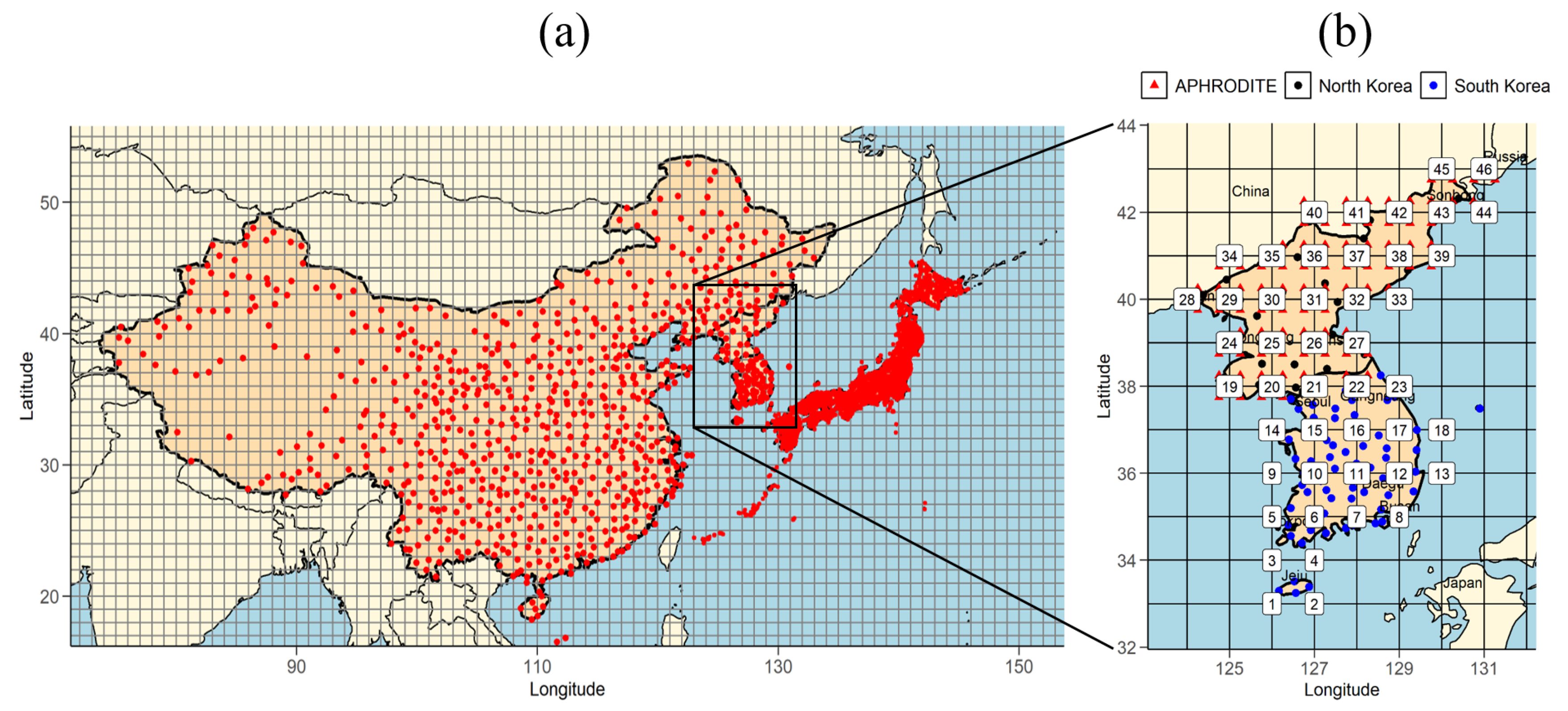
Figure 1. (a) Map of East Asia showing the observations sites and grid points. The Barnes interpolation method was employed to re-grid and to construct a rainfall field over 1 × 1 grids of 1180 points over East Asia. (b) Map of the Korean peninsula from 123 to 132 longitude and 33 to 43 latitude, including the sea and land, with 46 grid points of 1 × 1 for this study.
Atmosphere 12 00097 g001
Figure 2. Plot of the entropy as σ S changes from 0.1 to 1.0 and the selected σ S = 0.4 .
Atmosphere 12 00097 g002
Figure 3. Plot of the chi-square statistic values for the annual maximum daily precipitation (AMP1) as σ D changes. The selected σ D is 0.17 (0.19) for the p-value 0.05 (0.01).
Atmosphere 12 00097 g003
Figure 4. A graphical representation of the intermodel distance matrix for the 21 Coupled Model Inter-Comparison Project Phase 6 (CMIP6) models obtained from the five climate variables for East Asia. Each box represents a pairwise combination, where red colors indicate a greater independence and blue colors indicate a greater similarity.
Atmosphere 12 00097 g004
Figure 5. Spread of the weights for the 21 CMIP6 models obtained based on the performance only, the independence only, and both the performance and independence. The weights are obtained from the five climate variables for East Asia.
Atmosphere 12 00097 g005
Figure 6. Time series plots of the nine-year moving averages of the annual maximum daily precipitation in Seoul from the observations (red line) and from the PI-weighted ensemble of the bias-corrected historical data (black line) of the 21 CMIP6 models for the past years (1953–2014) and the PI-weighted ensembles for the bias-corrected future data from the three shared socioeconomic pathway (SSP) scenarios, with a 90% confidence band. The blue line is for SSP2-4.5, the green line is for SSP3-7.0, and the red line is for SSP5-8.5.
Atmosphere 12 00097 g006
Figure 7. Schematic boxplots of 20-year return levels (unit: mm) of the annual maximum daily precipitation averaged over 46 grids in the Korean peninsula for the future periods, i.e., P1 (2021–2050), P2 (2046–2075), and P3 (2071–2100), under the SSP2-4.5, SSP3-7.0, and SSP5-8.5 scenarios. OBS and HIST(NBC) indicate the observations and the historical data without a bias correction. The boxplot for P0 represents the bias-corrected historical data.
Atmosphere 12 00097 g007
Figure 8. Isopluvial maps of the 20-year return levels (unit: mm) of the annual maximum daily precipitation for 46 grids over the Korean peninsula for the future periods: P1 (2021–2050), P2 (2046–2075), and P3 (2071–2100) under the SSP2-4.5, SSP3-7.0, and SSP5-8.5 scenarios.
Atmosphere 12 00097 g008
Figure 9. Parallel coordinated boxplots, similar to those in Figure 7, but for 20- and 50-year return periods relative to the observations from 1973 to 2010.
Atmosphere 12 00097 g009
Figure 10. Bar plots (unit: %) representing uncertainties in projecting future climate or the variations owing to the models, scenarios, model and scenario interaction, and residuals for 20-year return levels over the Korean peninsula for each period.
Atmosphere 12 00097 g010
Figure 11. Interaction plots of the 20-year return levels from the 21 CMIP6 models for three SSP scenarios averaged over three periods and 46 grids in the Korean peninsula.
Atmosphere 12 00097 g011
Figure 12. Interaction plots of the 20-year return levels from the 21 CMIP6 models for three SSP scenarios for each period (P1, P2, and P3).
Atmosphere 12 00097 g012
Figure 13. Boxplots of the 20-year return levels (unit: mm) from the 21 CMIP6 models as the latitude changes from 35 to 42 . The solid lines around the boxes across the latitude are the spatial medians of 20-year return levels for each latitude and for P0 (1973–2010, i.e., the observation period), P1 (2021–2050), P2 (2046–2075), and P3 (2071–2100). The dashed lines depict those values for the three scenarios (SSP2-4.5, SSP3-7.0, and SSP5-8.5).
Atmosphere 12 00097 g013
Figure 14. Scatter plot showing the differences of variances of the 20-year return levels calculated from the PI-weights and the equal weights, plotted for 46 grid points in the Korean peninsula for each future period and for each scenario. V a r P I for the Y-axes (top panel) is the variance calculated by (13) from the PI-weights, and V a r B M , P I (middle panel) and V a r W M , P I (bottom) are the between-model and within-model variances, respectively. V a r E q , V a r B M , E q , and V a r W M , E q for the X-axis are the corresponding variances calculated from the equal weights. The value on each point in the top panel is a sum of those in the middle and in the bottom panels.
Atmosphere 12 00097 g014
Table 1. The five climate variables considered in this study.
Variable AcronymDescription
AMP1Annual Maximum Daily Precipitation
AMP5Annual Maximum Five-Day Precipitation
ATPAnnual Total Precipitation
AMCWDAnnual Maximum Consecutive Wet Days
AMCDDAnnual Maximum Consecutive Dry Days
Table 2. The expected waiting time (unit: year) until reoccurrence or the return period of specific annual maximum daily precipitation (AMP1) values from 100 to 500 mm in the Korean peninsula obtained from the observations (OBS) and the CMIP6 model ensemble under the three SSP scenarios for the three future periods (P1, P2, and P3).
SSP2-4.5SSP3-7.0SSP5-8.5
AMP1OBSP1P2P3P1P2P3P1P2P3
100 mm1.81.41.31.31.41.31.21.41.31.2
150 mm4.44.43.93.74.03.22.53.63.02.5
200 mm11.114.511.110.613.210.27.113.08.05.9
250 mm30.741.731.727.142.928.716.934.424.915.0
300 mm789376551045942765029
400 mm485400297202469254201227166107
500 mm197011678145771148649563538493307
Table 3. The 20-year return levels (unit: mm) of the annual maximum daily precipitation (AMP1) and of the annual maximum five-day precipitation (AMP5) averaged over each latitude for the observations (OBS) during 1973–2010 and for future periods—namely, P1 (2021–2050), P2 (2046–2075), and P3 (2071–2100). For each future period, the values were averaged over the three scenarios.
20-Year Return Level (AMP1)20-Year Return Level (AMP5)
LatitudeOBS P 1 P 2 P 3 OBS P 1 P 2 P 3
33288303319345443440471519
34275288303329416416446487
35253264280305384386412445
36235246261282360368389414
37243252270296396409429461
38249262281302402419438466
39227245267287377398417442
40186209227247299319337357
41147166181201236249266285
42136149164181207213235250
43143151167184223227254271
Table 4. The averaged values of the Brier skill scores (BSSs), averaged differences of variances (unit: mm 2 ) of the 20-year return level over 46 grid points in the Korean peninsula, and relative improvements (RIs) of the PI-weighted method over the simple average (last column) for the three periods and for the three scenarios. RI = V E q V P I V P I × 100 . D V = V a r E q V a r P I , D V B M = V a r B M , E q V a r B M , P I , and D V W M = V a r W M , E q V a r W M , P I . Other acronyms are the same as in Figure 14.
ssppBSS(%) BSS BM BSS WM DV DV BM DV WM RI(%)
P1−2.2−12.32.0−50−7727−3.3
SSP2-4.5P27.719.73.212982478.5
P313.439.02.73092674217.1
P117.942.95.43002386224.0
SSP3-7.0P211.022.54.722815375.013.7
P316.736.21.44263784819.5
P16.424.7−4.5113138−258.0
SSP5-8.5P210.433.9−6.9178291−1138.0
P322.542.2−1.1826834−826.0
Publisher’s Note: MDPI stays neutral with regard to jurisdictional claims in published maps and institutional affiliations.