Optimal Estimation MSG-SEVIRI Clear-Sky Total Column Water Vapour Retrieval Using the Split Window Difference

Abstract

A new algorithm for the retrieval of day-time total column water vapour (TCWV) from measurements of a MSG-SEVIRI (Meteosat Second Generation Spinning Enhanced Visible and Infrared Imager) instrument is presented. The retrieval is based on a forward operator, at the core of which lies Radiative Transfer for TIROS Operational Vertical Sounder (RTTOV). This forward model relates TCWV and surface temperature to brightness temperatures in the split window at 11 and 12µm with the use of a first guess for temperature and humidity profiles from the ERA5 reanalysis. The forward model is then embedded in a full Optimal Estimation (OE) method, which yields pixel by pixel uncertainty estimates and performance indicators. The algorithm is applicable to any instrument which features the split window configuration, given a first guess for atmospheric conditions (i.e., from NWP) and an estimate of surface emissivity at 11 µm. The algorithm was developed within the framework of RealPEP (Near-Realtime Quantitative Precipitation Estimation and Prediction) in which the advancement of the estimation and nowcasting of extreme precipitation and flooding in Germany are studied. Thus, processing and validation has been limited to the German domain. Three independent ground-based TCWV observation data sets were used as reference, i.e., AERONET (Aerosol Robotic Network), GNSS Germany (Global Navigation Satellite System) and measurements from two MWR (Microwave Radiometer) sites. The validation concludes with good agreement, with absolute biases between 0.11 and 2.85 kg/m${}^2$, root mean square deviations (rmsds) between 1.63 and 3.24 kg/m${}^2$ and Pearson correlation coefficients ranging from 0.96 to 0.98. The retrievals uncertainty estimates were evaluated against AERONET. The comparison suggests that, in sum, uncertainties are estimated well, while still some error sources seem to be over- and underestimated. In limited case studies it could be shown that SEVIRI TCWV is capable to both display large scale variabilities in water vapour fields and reproduce the daily course of water vapour exposed by ground-based observations.

1. Introduction

Water vapour is one of the most abundant trace gases in the atmosphere. The evaporation of water and the transport of water vapour in the atmosphere play an integral role in the global hydrological cycle [1]. In processes referred to as so-called atmospheric rivers water masses equivalent to big rivers are transported across the globe [2]. In combination with aerosols, water vapour is fundamental to the formation of clouds and, subsequently, precipitation. Water vapour influences boundary layer processes such as convection initiation [3,4] and its long and short-term variability is directly linked to high-impact phenomena such as droughts, severe thunderstorms and high precipitation events [3,4,5,6]. Due to its strong absorption of electromagnetic radiation, water vapour is also the most efficient greenhouse gas in the atmosphere [1,7]. Coupled with the influence of clouds on the earth’s radiative budget [8], an atmosphere with increasing water vapour holding capacity [8,9] and changing weather patterns, the net influence of water vapour on climate change is both important and difficult to quantify. It becomes clear that water vapour is a trace gas that needs to be monitored closely. The Global Climate Observing System (GCOS) declared total column water vapour (TCWV) as a critical variable for the characterisation of the climate system and its changes [10]. TCWV describes the mass of integrated atmospheric humidity, if the total column of it would condense and precipitate over a unit cross-section and is measured in [kg/m${}^2$], [mm] or [cm]. The standard long name for TCWV as defined by the climate and forecast (CF) Metadata Conventions is atmosphere water vapour content [11]. In the literature, different terms and abbreviations can be found to describe TCWV such as total water vapour content (TWC), total water vapour (TWV), integrated water vapour (IWV), precipitable water (PRW), precipitable water vapour (PWV) or total precipitable water (TPW). In this study, we will exclusively use TCWV and the unit [kg/m${}^2$].

In the past decades, a multitude of space- and ground-based retrieval methods for TCWV have been developed. Most broadly available, satellite-based TCWV retrievals work in the visible (e.g., Global Ozone Monitoring Experience (GOME) [12], Scanning Imaging Absorption Spectrometer for Atmospheric Chartography (SCIAMACHY) [13]) in the near-infrared (NIR) (Medium Resolution Imaging Spectrometer (MERIS) [14], Moderate Imaging Spectrometer (MODIS) [15], Ocean and Land Colour Instrument (OLCI) [16]), the infrared (IR) (e.g., Infrared Atmospheric Sounding Interferometer (IASI) [17]) or the microwave spectrum (Special Sensor Microwave Imager (SSMI), Special Sensor Microwave Imager Sounder (SSMI/S) [18]), but are limited to polar-orbiting satellites. Geostationary satellites regularly include channels at 6 and 7 µm in order to quantify outgoing long wave radiation and water vapor in the upper troposphere via the thermal emissions of water vapour at these wavelengths [19,20]. However, these methods are insensitive to the water vapour in the boundary layer below 850 hPa geopotential height even though it contains the predominant part of the integrated humidity.

An alternative are the so-called split window bands near 11 and 12 µm, which were originally introduced to improve surface temperature retrievals. These are sensitive down to the bottom-of-atmosphere. Previous studies already investigated and developed a wide array of different retrievals of TCWV exploiting the split window [21,22,23,24,25,26,27]. For instance, the approach proposed in [21,22,24] is based on the assumption that a ratio of transmittance in each of the split windows can be approximated. This ratio can then be related to true TCWV (e.g., from radiosondes). The regression fit from this relation is used to retrieve TCWV. This procedure has the benefit that no a priori knowledge or first guess is needed. The Physical Split Window technique (PSW) used in [23,27,28] is built on a perturbation formulation of a simplified radiative transfer equation. A first guess from observation data or numerical weather prediction (NWP) is then taken and the equation solved together with the split window observations to retrieve T${}_{skin}$ and TCWV. PSW TCWV is in operational use for the FengYun-2 (FY2) [28]. In contrast to the other approaches, the Advanced Infrared Water Vapour Estimator (AIRWAVE) works explicitly over ocean [26]. It exploits the dual-view split window (forward and nadir) of the Along Track Scanning Radiometer (ATSR), advanced radiative transfer and a sea surface emissivity data base to retrieve day- and night-time clear sky TCWV over oceans. Furthermore, the simple difference between split window bands—the Split Window Difference (SWD)—is used as an indicator for atmospheric conditions in relation to moisture content [29,30].

Opposed to the other retrievals, the approach taken in this study is based on the full iterative optimal estimation (OE) technique and will use a radiative transfer model (RTM) as a forward operator. At each step of the iteration Top-of-Atmosphere (TOA) brightness temperatures (BT) are simulated starting from a first guess of TCWV and surface temperature T${}_{skin}$, atmospheric profiles from NWP and a surface emissivity data set. In theory, this allows for improved retrieval of day- and night-time TCWV and T${}_{skin}$ over both ocean and land surfaces. Another benefit is that OE provides a rigorous uncertainty estimate for the retrieved parameters. This includes performance indicators such as the cost function, averaging kernels which will be explained in more detail. In addition to that, the OE allows for the quantification of sensitivities (e.g., influence of inversions, dust, etc.), and the algorithm can easily be extended for the use of additional channels as well as the estimation of additional geophysical parameters.

We provide this algorithm for use on the Spinning Enhanced Visible and InfraRed Imager (SEVIRI) onboard the geostationary satellites Meteosat Second Generation (MSG). However, our retrieval is also seamlessly adaptable to other satellites which feature a similar band configuration, e.g., Advanced Along Track Scanning Radiometer (AATSR), Advanced Very High Resolution Radiometer (AVHRR), Feng-Yun2 (FY2), Geostationary Operational Environmental Satellite (GOES), MODIS, and Sea Land Surface Temperature Radiometer (SLSTR), just to name a few.

The work presented here is performed within the German project of the Near-Realtime Quantitative Precipitation Estimation and Prediction (RealPEP) [31,32]. The project is a cooperative work between various institutes across several fields of research (radar meteorology, hydrology, numerical weather predictions, remote sensing) in order to improve the quantification and nowcast of extreme precipitation and floods in Germany. Knowledge about the amount of TCWV on sub-daily or sub-hourly timescales and at spatial scales that allow the observation of small-scale (convective) structures in the TCWV field can vastly expand the understanding and prediction of precipitation (e.g., description of the pre-convective environment before the onset of cloud formation and precipitation). The presented algorithm should be applicable globally, both over land and water surfaces. With RealPEP’s focus on Germany, the retrieval and the validation of the TCWV product was limited to Germany and land surfaces.

The structure of this paper is as follows: In Section 2, we first present SEVIRI, the algorithm basis and method as well as the data used in the retrieval and introduce the three reference data sets. The validation against these references and the uncertainty evaluation, followed by application examples of the retrieval, can be found in Section 3. Finally, the results are discussed in Section 4.

2. Data and Methods

2.1. MSG SEVIRI

SEVIRI is the main instrument of the EUMETSAT’s (European Organisation for the Exploitation of Meteorological Satellites) MSG, which is at an altitude of 36,000 km. MSG is the successor of Meteosat First Generation (MFG). SEVIRI is a 50 cm diameter aperture, line by line scanning radiometer. It provides image data in four visible and near-infrared channels and eight infrared channels. The algorithm presented in this paper only uses the two infrared channels 9 (10.8 µm) and 10 (12.0 µm), see

Table 1. SEVIRI bands used in the TCWV retrieval and their associated characteristics [19].

Band	$\mathit{\lambda }$ (µm)	Width (µm)	Spec. Noise (K)	Main Applications
9	10.8	2	0.25	sea and land surface temperature, cloud top temperatures
10	12	2	0.37	sea and land surface temperature, cloud top temperatures

for the detailed specifications. These two bands feature a spatial resolution of 3 km (sampling distance) at sub-satellite point. Each single scan is done with 3 band detection elements per channel. The full disk is captured after 1250 scan lines with a 9 km sub-satellite-pixel (ssp) per line step. Full disk scanning is achieved by spinning the satellite at 100 revolutions per minute and it is completed after 12.5 min. After calibration with an onboard black body and retracing, earth observation is resumed. This leads to an overall repeat cycle of 15 min and yields a 3750 by 3750 pixel images (for channel 9 and 10). More detailed information on the workings of SEVIRI can be found in [19,33]. The measurements used in this paper are High Rate SEVIRI Level 1.5 Image Data [34] from MSG3 at 0${}^{\circ }$. The data have been accessed and downloaded from the EUMETSAT Data Store [35]. The spatial resolution over Germany is approximately 3.3 km (zonal) by 6 km (meridional).

2.2. Physical Background

Water in the gaseous phase exhibits varying absorption of electromagnetic radiation across a wide range of wavelengths. These variations stem from a combination of three fundamental vibration modes, their overtones and rotational transitions of the water molecule. It is assumed that the difference between measurements of emitted brightness temperatures (BT) within the far-infrared at the 10 µm through in the water vapour absorption spectrum provide information about the integrated water vapour content.

In the far-infrared, scattering is negligible, since the wavelengths we measure at are much larger compared to average aerosol sizes. However, larger particles in cases such as desert dust outbreaks or thin cirrus clouds can contaminate our measurements. Thus, the retrieval is strictly limited to clear-sky conditions only.

Radiative transfer is based on the Schwarzschild’s equation in a non-scattering medium which reads (e.g., [36]):

$$I_{TOA}=I_{BOA}·{\tau }_{(0-s_{TOA})}+\int B\left(s\right)·W\left(s\right)ds$$

(1)

The top-of-atmosphere (TOA) radiance for far-infrared brightness temperatures $I_{TOA}$ [K] is made up of the bottom-of-atmosphere (BOA) radiance $I_{BOA}$ [K] multiplied with the atmospheric transmittance $\tau (0-s_{TOA})$ [1] and the integral of the emitted radiation $B\left(s\right)$ from the layer s multiplied with the weighting function $W\left(s\right)$, which is mainly influenced by the humidity in layer s.

In sum, our retrieval is limited to the following conditions:

• The absorption measuring band is located in a sensitive part, but is not saturated;
• The surface emissivity and surface temperature can be estimated;
• The troposphere is not masked by any clouds (this includes thin cirrus) nor thick aerosol layers of large particle sizes.

This would yield us a daytime (and, theoretically, night-time), clear-sky TCWV retrieval over land and ocean surfaces. However, prior knowledge about the profile of temperature and humidity and a layer-by-layer radiative transfer simulation is required.

2.3. The Algorithm Core

Our retrieval is based on the full Optimal Estimation (OE) approach as described in [37]. This technique optimises the difference between simulated and measured radiances (BTs in this case) by varying state parameters iteratively [16,38]. In our case, the state parameters are the TCWV and the surface temperature (T${}_{skin}$). The retrieval uncertainties are estimated from all known uncertainty influences, e.g., instrument noise, parameter uncertainties, etc.

Starting from a first guess for our state, we calculate the state of the next step as follows:

$$x_{i+1}=x_i+\left(G(y-F\left(x_i\right))\right)$$

(2)

where x is the state at step i, y is the measurement, $F\left(x_{*}\right)$ is the simulated measurement with F being the forward operator and G is the gain. The gain describes how each measurement contributes to each element in the retrieved state. G is calculated as follows:

$$G=S_a{K}^T{(K{S}_a{K}^T+S_e)}^{-1}$$

(3)

$S_e$ and $S_a$ are the measurement and a priori error covariance matrices, respectively. K is the Jacobian matrix which contains the partial derivatives of each of the measurements relative to each of the states, i.e., $K=\partial y/\partial x$. The optimal state of x can be estimated by minimising the cost function $J\left(X\right)$. The cost function reads:

$$J\left(x\right)=1/2{(y-F\left(x\right))}^T{S_e}^{-1}(y-F\left(x\right))+1/2{(x_a-x)}^T{S}_a^{-1}(x_a-x)$$

(4)

This approach is based on the assumptions that uncertainties follow Gaussian probability functions and that measurements, a priori knowledge and forward model are bias free. There are several possibilities to solve Equation (3). We chose Gauss–Newton.

Convergence is reached and the iteration stopped when the maximum number of iterations is reached or when the following criterion is met. This would mean that the left part of Equation (5) is magnitudes smaller than the number of retrieved states ($<<n$):

$${(x_i-x_{i+1})}^T·S_i^{-1}·(x_i-x_{i+1})<=n*ϵ$$

(5)

n is the number of parameters in the state vector and $ϵ$ is adjustable, e.g., 0.01. S is the retrieval error covariance, it also contains the uncertainties of our retrieved state and will be examined in more detail in Section 2.4.

Since this OE approach is developed for linear problems, a useful step to speed up the convergence process is to transform the measurement so that the relationship between measurement and state becomes more linear. Thus, the measurement vector for this algorithm does not simply consist of our measurements at 10.8 and 12 µm, but rather in correspondence with our state (TCWV, T${}_{skin}$) to a difference between window channel and absorption channel (i.e., BT${}_{11}$, BT${}_{11}$–BT${}_{12}$). This is the so-called Split Window Difference (SWD).

The gain matrix can also be expressed as the partial derivative of the true state $\partial \widehat{x}$ in relation to the partial derivative of the measurement $\partial y$. The true state $\widehat{x}$ is unknown. However, via the relative changes at each step, we can quantify the sensitivity of it towards changes in y, following Equation (3). By combining G with the Jacobian K, we receive an estimate of how far the retrieved state x represents the true state $\widehat{x}$. The matrix product of G and K yields the so-called Averaging Kernel A (AVK):

$$A=G·K=\frac{\partial \widehat{x}}{\partial x}$$

(6)

Ideally, the entries along the diagonal of A show a range of values between 0 and 1. At 0, the proportion of the retrieved state at $\widehat{x}$ is lowest, the measurement did not contribute to the retrieval. In that case, the solution comes purely from the prior knowledge. At 1, the proportion of the retrieved state at the true state is highest. The a priori information plays no or a minor role. Everything in between indicates that some improvement of the prior information about the state could be made using the information from the measurement.

2.4. Uncertainty Estimation

One benefit of the OE approach is that input uncertainties are propagated through each step and provide a good uncertainty estimate at the final step. All relevant sources of uncertainty such as sensor noise, errors of forward modelling parameters and the prior knowledge need to be accounted for. In order to consider uncertainties introduced by the forward model, $S_e$ is composed from the error covariance matrix of the measurement $S_y$ (i.e., specified instrument signal noise) and from the forward model parameter error co-variance matrx $S_B$. $K_B$ is the Jacobian of the forward model F against the parameterisations B.

$$S_e=S_y+{K_B}^T{S}_B{K}_B$$

(7)

The retrieval uncertainty $\widehat{S}$ is part of each iteration step (Equations (2) and (3)):

$$\widehat{S}={({S_a}^{-1}+{K_i}^T·{S_e}^{-1}·K_i)}^{-1}$$

(8)

The uncertainty of a priori TCWV is taken to be 20% of the a priori TCWV value. T${}_{skin}$ is computed from BT${}_{11}$ and emissivity ${\epsilon }_{11}$, following Rayleigh Jeans law. Thus, the uncertainty of T${}_{skin}$ is calculated from the square root of the sum of the squares of the uncertainty of ${\epsilon }_{11}$ and the uncertainty of BT${}_{11}$ (i.e., instrument noise).

2.5. Forward Operator: RTTOV

In order to simulate measured TOA BTs at each step in the retrieval, a RTM is needed. Any RTM that is capable of simulating in the spectral range of the split window should be applicable (e.g., CRTM, MODTRAN, RTTOV). The forward model chosen for this retrieval is the Radiative Transfer for TIROS Operational Vertical Sounder (RTTOV) version 12 [39]. RTTOV is a fast and flexible radiative transfer model (RTM) for a wide range of wavelengths and sensors. This is done by using coefficient files, which are provided for a wide range of platforms (i.e., AVHRR, GOES, FY2, HIMAWARI, Meteorological Operational Satellite (METOP), SLSTR, etc.) and which can be easily adapted within the structure of this algorithm. RTTOV is widely used in an operational environment, i.e., the Satellite Application Facility on Climate Monitoring (CM SAF). For this retrieval, it was decided to practically “constrain” RTTOV to just two input parameters: the surface temperature (T${}_{skin}$) and the integrated humidity (TCWV).

Since RTTOV requires atmospheric profiles as input, humidity profiles are provided which have been scaled with the previous estimate of TCWV for each iterative step. The form of the profile is kept constant under the assumption that the first guess humidity profile reflects the true shape. However, it is scaled such that the integrated humidity equals the OE estimate at iteration step i. The temperature at the lowest profile layer $T_{profile}\left(p_{max}\right)$ and the 2 m Temperature $T_{2m}$ are adapted with T${}_{skin}$. The optional ozone profile as input is not used for now (see

Table 2. Overview of parameters passed on to RTTOV, which change during each iterative step and their calculation.

Updated Parameter	Calculation
$T_{profile}(p_{max},i+1)$	$T_{skin,i}-\left(T_{profile}(p_{max},i)-T_{skin,i}\right)$
$T_{2m,i+1}$	$T_{skin,i}-\left(T_{2m,i}-T_{skin,i}\right)$
$q_{profile}(i+1)$	$(TCW{V}_i$/${\int }_0^{p_{min}}q\left(p\right))·q_{profile}\left(i\right)$
$q_{2m}(i+1)$	$(TCW{V}_i$/${\int }_0^{p_{min}}q\left(p\right))·q_{profile}(i,p=p_{max})$

). RTTOV is operated in a vectorised and parallelised configuration in order to keep the computation time for a whole scene retrieval as low as possible. For this study reanalysis data from ECMWF’s (European Centre for Medium-Range Weather Forecasts) ERA5 reanalysis, accessed via the Copernicus Climate Change Service (C3S) Climate Data Store (CDS) [40], have been used. In an operational mode, the source of temperature and humidity profiles will be taken from NWP forecasts.

2.6. Input Data

The retrieval uses brightness temperatures measured in K. The SEVIRI channels 9 and 10, which are typically used as atmospheric windows for the retrieval of surface temperatures [20,41], were chosen (see

Table 3. All inputs for the algorithm, their assigned variables (+ description), sources and units used.

Assigned Vector	Description/ Variable	Source/ Calculation	Unit
X${}_a$	TCWV	ERA5 reanalysis	[kg/m${}^2$]
	T${}_{skin}$	$B{T}_{11}·{\epsilon }_{11}$	[K]
S${}_a$	${\sigma }_{TCWV}$	${(0.2·x_{a,TCWV})}^2$	[1]
	${\sigma }_{T_{skin}}$	$\left(\frac{B{T}_{11}}{{\epsilon }_{11}}·\sqrt{{\frac{B{T}_{11}}{{ϵ}_{B{T}_{11}}}}^2+{\frac{{\epsilon }_{11}}{{ϵ}_{{\epsilon }_{11}}}}^2}\right)$	[1]
Y	$B{T}_{11}$	SEVIRI channel 9	[K]
	$B{T}_{11-12}$	SEVIRI channel 9 - SEVIRI channel 10	[K]
S${}_e$	${\sigma }_{B{T}_{11}}$	${ϵ}_{B{T}_{11}}^2+{ϵ}_{F{\left(B\right)}_{11}}^2$	[1]
	${\sigma }_{B{T}_{11-12}}$	${ϵ}_{B{T}_{11-12}}^2+{ϵ}_{F{\left(B\right)}_{11-12}}^2$	[1]
p	longitude	SEVIRI	[${}^{\circ }$E]
	latitude	SEVIRI	[${}^{\circ }$N]
	elevation	NASA’s Shuttle Radar Topography Mission (SRTM) [44]	[km]
	viewing zenith angle	SEVIRI	[${}^{\circ }$]
	sun zenith angle	SEVIRI	[${}^{\circ }$]
	${\epsilon }_{11}$ (emissivity)	MYD11C2 (MODIS AQUA)	[1]
	${\epsilon }_{12}$ (emissivity)	MYD11C2 (MODIS AQUA)	[1]
	T${}_{skin}$	s.a., upddated with T${}_{skin}$	[K]
	T${}_{2m}$ (temperature at 2 m)	ERA5 reana., updated with T${}_{skin}$ from X${}_a$ or previous step	[K]
	q${}_{2m}$ (humidity at 2 m)	ERA5 reana., updated with TCWV from X${}_a$ or previous step	[ppmv]
	wind${}_u$ (zonal wind)	ERA5 reana.	[m/s]
	wind${}_v$ (meridional wind)	ERA5 reana.	[m/s]
	T${}_{profile}$ (temperature profile)	ERA5 reana., T${}_0$ updated with T${}_{skin}$ from X${}_a$ or previous step	[K]
	q${}_{profile}$ (humidity profile)	ERA5 reana., updated with TCWV from X${}_a$ or previous step	[ppmv]
	p${}_{profile}$ (pressure levels)	ERA5 reana.	[hPa]

). These are also referred to as Atmospheric Split Window.

The a priori of TCWV in $x_a$ is taken from the ERA5 reanalysis. T${}_{skin}$ in $x_a$ is computed from SEVIRI’s BT${}_{11}$ and emissivity ${\epsilon }_{11}$ from the MODIS AQUA 8-day emissivity product (MYD11C2) [42]. Pixel-based ${\epsilon }_{11}$ uncertainty provided by the MYD11C2 product is used for the uncertainty estimation described in Section 2.4. The a priori vector is also taken as the first guess $x_{i=0}$ for the start of the OE.

All of the other parameters provided to the forward model are listed in Table 3. The parameters do not change throughout the iteration, except for the ones listed in Table 2. At $i=0$$T_{profile}\left(p_{max}\right)$ is calculated from $T_{skin,i}-\left(T_{profile}(p_{max},era5)-T_{skin,era5}\right)$ and $T_{2m}$ is computed from $T_{skin}-\left(T_{2m,era5}-T_{skin,era5}\right)$. For $q_{profile}$ and $q_{2m}$ at $i=$ 0, the scaling factor is 1.

Since this new water vapour retrieval algorithm is developed within the framework of the RealPEP project which focuses on advancing the nowcasting of (extreme) precipitation and flash flood events in Germany, the processing and the validation of this algorithm is limited to the German domain (4.5–15${}^{\circ }$ longitude, 45–55${}^{\circ }$ latitude). The retrieval was performed for a subset of the 15 min SEVIRI full disk between 6 a.m. and 11 p.m. for 26 days in total, which were identified as clear- or semi-clear-sky days over the whole domain. Furthermore, some days within specific study periods set by the RealPEP project have been processed and validated. This selective processing resulted in nearly 3000 scenes in total for several days between January and October 2017. The MSG cloud mask from the MSG-SEVIRI-based cloud property data record Cloud Property Dataset using SEVIRI, Edition 2 (CLAAS-2) [43] was used for cloud screening (i.e., MSG Cloud Physical Properties MSGCPP). Pixels marked as clouds or cloudy by MSGCPP were excluded from the processing for each scene.

2.7. Reference Data Sets

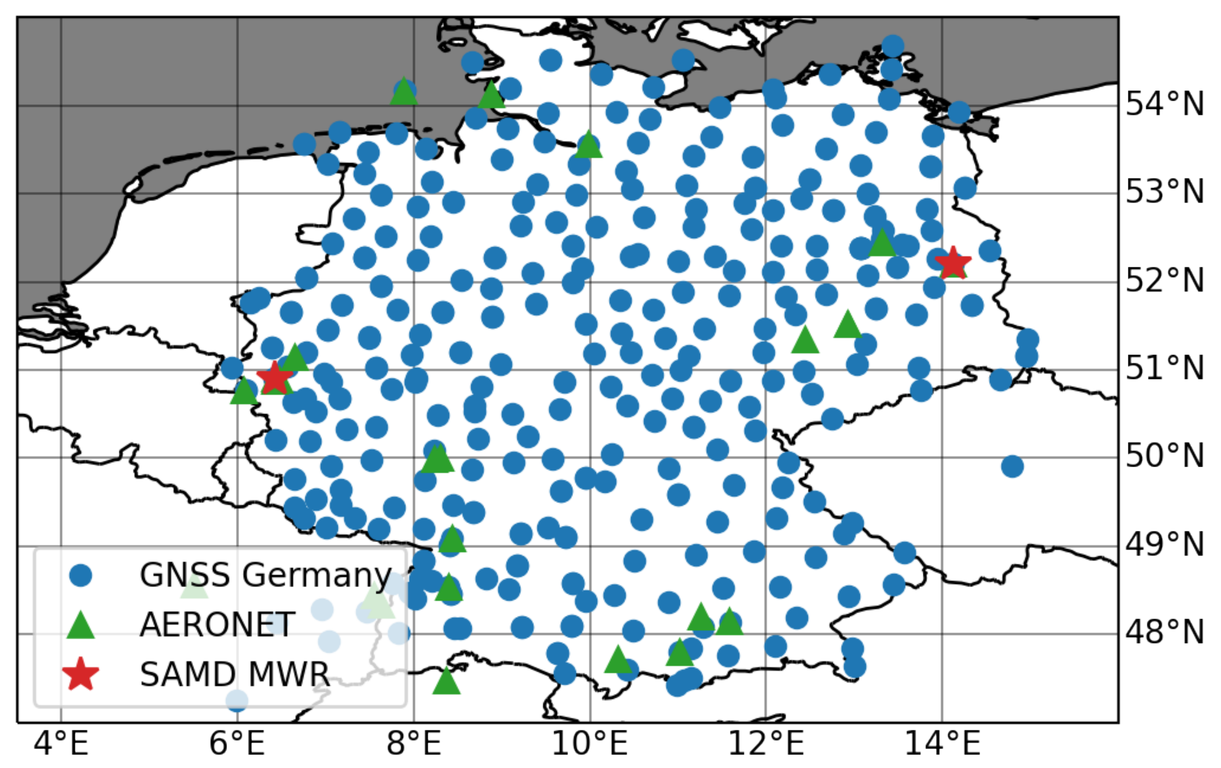
In order to validate this new algorithm and its product, we collected TCWV observations from several networks and ground-based stations which operated in Germany at the time of satellite observations. We performed a validation of the product against ground-based measurements of the Aerosol Robotic Network (AERONET), the Global Navigation Satellite System (GNSS) and several German microwave radiometric stations. The study domain and the positions of the used reference data sets are shown in Figure 1.

2.7.1. AERONET

Several AERONET stations are located in and around Germany. The network’s main goal is long-term observations of aerosol optical properties and precipitable water with stations around the globe. Direct-sun photometer instruments measure downwelling radiances within the rho-sigma-tau absorption band, which are then converted to the aforementioned variables [45]. Temporal resolution and data availability depends on weather conditions and the scan settings and can vary between 2 and 20 min during sun light. For this study, we use the Algorithm Version 2 [46]. AERONET TCWV exhibits a consistent dry bias of approx. 5–6% and an estimated uncertainty of 12–15% [47]. Data were downloaded from the network’s website [48] and binned into 15 min intervals in order to be matched up with SEVIRI’s 15 min observations.

2.7.2. GNSS Germany

In central Europe, a dense network of GNSS stations provide long-term observations of water vapour. Water vapour amounts are estimated from the travel times of signals from several GPS satellites to a receiver at the ground station. Humidity, as well as temperature cause delays in the signal and thus, the travel times can be related to TCWV [49,50]. The observations are not compromised by any weather conditions and provide water vapour every 15 min around the clock. The networks uncertainty is estimated to be between 1 and 2 kg/m${}^2$ [50,51]. The data set was downloaded from the Standardized Atmospheric Measurement Data (SAMD) Archive [52].

2.7.3. Microwave Radiometers in Germany

At several sites in Germany, ground-based microwave radiometers (MWR) are operated. The stations available for 2017 are the Jülich Observatory for Cloud Evolution (JOYCE) [53], the Meteorologisches Observatorium Lindenberg Richard-Aßmann-Observatorium (MOLRAO) and Umweltforschungsstation Schneefernerhaus (UFS). MWRs measure emitted radiation at several channels in the microwave spectrum within a narrow zenith looking angle. The measured brightness temperatures are used to retrieve TCWV via a multiple regression, which is developed for each site [54,55]. These instruments provide high-accuracy, high-temporally resolved water vapour estimates at any time of day and virtually any weather conditions given that the instrument is not covered with water. The temporal resolution is in the order of seconds and uncertainties are around 0.5–0.8 kg/m${}^2$ [56]. The data are provided by and were downloaded from the SAMD as well.

3. Results

3.1. Validation Study

Spatial and temporal match-ups between the MSG SEVIRI TCWV data set and the three reference TCWV data sets have been created. These cover clear-sky periods between January 2017 and October 2017.

The reference data sets have been filtered according to corresponding quality flags and averaged within 15 min time frames. A full disk scan by SEVIRI is done in 12 min and starts every full 15 min. SEVIRI TCWV was averaged over a 5 by 5 pixel (16.5 km by 30 km) area surrounding the matched up satellite pixel, provided the following criteria were met:

• 100% of satellite pixels are cloud free (the MSGCPP cloud mask was used).
• 90% of satellite pixels are valid (algorithm converged) and plausible (cost function < 2).
• The difference between the average of the digital elevation model (DEM) over the pixel area used for the forward modelling and the elevation of the reference station is less than 100 m.

The performance indicators used in this study are the bias, root mean square deviation (rmsd), the Pearson correlation coefficient ($r^2$) and offset $\alpha$ and slope $\beta$ from an orthogonal distance regression (ODR).

3.1.1. AERONET

In total, there were 1275 match-ups for the AERONET reference with 30 available stations. The validation study shown in Figure 2 concluded with a wet bias of 2.85 kg/m${}^2$, a rmsd of 3.24 kg/m${}^2$ and a Pearson correlation coefficient of 0.97. This wet bias is in correspondence with literature, since in comparison with other water vapour products, AERONET exhibits a dry bias [47]. The ODR yields an offset of −0.02 and a slope of 1.15. Overall, the products show good agreement.

3.1.2. GNSS Germany

The GNSS network contains more stations than AERONET in Germany, there are 44,906 match-ups with 333 stations spread across the whole study domain. We observe a small dry bias of −0.11 kg/m${}^2$, a rmsd of 2.07 kg/m${}^2$ and a $r^2$ of 0.96. The ODR indicates a very good agreement between SEVIRI and GNSS TCWV with a slope of 1.03 and an offset of −0.57.

3.1.3. SAMD MWR Germany

In the validation study against TCWV retrieved from MWR (Figure 3) we only used two stations with a total of 897 match-ups. The study concludes with a wet bias of 0.96 kg/m${}^2$, a rmsd of 1.63 kg/m${}^2$ and a correlation of 0.98. Overall, there is good agreement. The ODR computed offset of 1.90 is higher than for the other references, the slope is slightly better with 0.95.

Match-ups with the MWR station UFS were excluded due to the big difference between DEM elevation and the station’s elevation of over 500 m. The correlation between the two products is high ($r^2$ = 0.95, not depicted); however, the slope and offset from ODR deviate from the ideal 1:1 ($\alpha =0.54$, $\beta =2.30$).

3.2. Validation of Pixel-Based SEVIRI TCWV Uncertainty Estimates

Sayer et al. present a framework for the quality assessment of uncertainty estimates [57]. Their approach is based on the assumption that uncertainties follow Gaussian distributions. The uncertainty estimates from an algorithm can be tested for this with the help of a reference data set with coinciding retrieval errors.

Preferably the database contains many match-ups and covers all seasons, regions and possible meteorological conditions. Out of the three reference data sets, AERONET is the only one that provides a relative uncertainty per measurement (Section 2.7.1). The network is inherently cloud-masked [58] and covers the processed region with 30 stations fairly well. For the evaluation of the SEVIRI TCWV uncertainty, the match-ups with AERONET over Germany is used.

In principle, this analysis compares the observed difference between the retrieved values and the reference, the absolute retrieval error (i.e., $\mid TCW{V}_{SEVIRI}-TCW{V}_{AERONET}\mid$) with a so-called total expected discrepancy (${ϵ}_{tot}$). ${ϵ}_{tot}$ is calculated from the square root of the sum of all available uncertainties squared under the assumption that all of these are independent of each other. In this case, these are the uncertainties from the SEVIRI TCWV retrieval, and AERONET TCWV multiplied with the maximum relative error estimate (15%). To account for sources of uncertainty in the match-ups themselves, measures for temporal variability and spatial variability are needed. Variability introduced by AERONET TCWV is represented by the standard deviation of TCWV within 15 min of the SEVIRI observation. Variability introduced by SEVIRI TCWV is represented by the standard deviation of SEVIRI TCWV within the 5 × 5 tiles around the AERONET station. From this follows:

$${ϵ}_{tot}=\sqrt{{{ϵ}_{SEVIRI}}^2+{{ϵ}_{AERONET}}^2+{{\sigma }_{SEVIRI}}^2+{{\sigma }_{AERONET}}^2}$$

(9)

In the next step, all ${ϵ}_{tot}$ are sorted into bins of 0.5 kg/m${}^2$, assuring an equivalent number of samples per bin across all bins through random selection from all available match-ups. For each bin, the 38th, 68th and 95th percentiles are calculated from the contained population. Following a Gaussian distribution, these percentiles relate to 0.5, 1 and 2 standard deviations, respectively. In an ideal case, the percentiles would follow each of the coloured lines in Figure 4.

Absolute retrieval errors increase with total expected discrepancy and follow the general direction of the ideal curves. For the 38th percentile, uncertainties in the lower area (1.5–3 kg/m${}^2$) align well, in higher areas; however, uncertainties are lower than observed, which indicates underestimation or ignorance of error sources. For the 68th, the absolute discrepancies are following the ideal curve well almost throughout the whole data range, which indicates a good error estimation. Since the performance in the 68th percentile directly relates to the expectation of the retrieval error of one standard deviation, the results are especially encouraging. In the 95th percentile, the retrieval errors seem to be overestimated. However, some sources of uncertainty seem to be overestimated since intermediate uncertainties (between 3.5 and 4.5 kg/m${}^2$) and absolute retrieval error drops against ${ϵ}_{tot}$.

3.3. Comparison of SEVIRI TCWV against High-Resolved COWa NIR TCWV

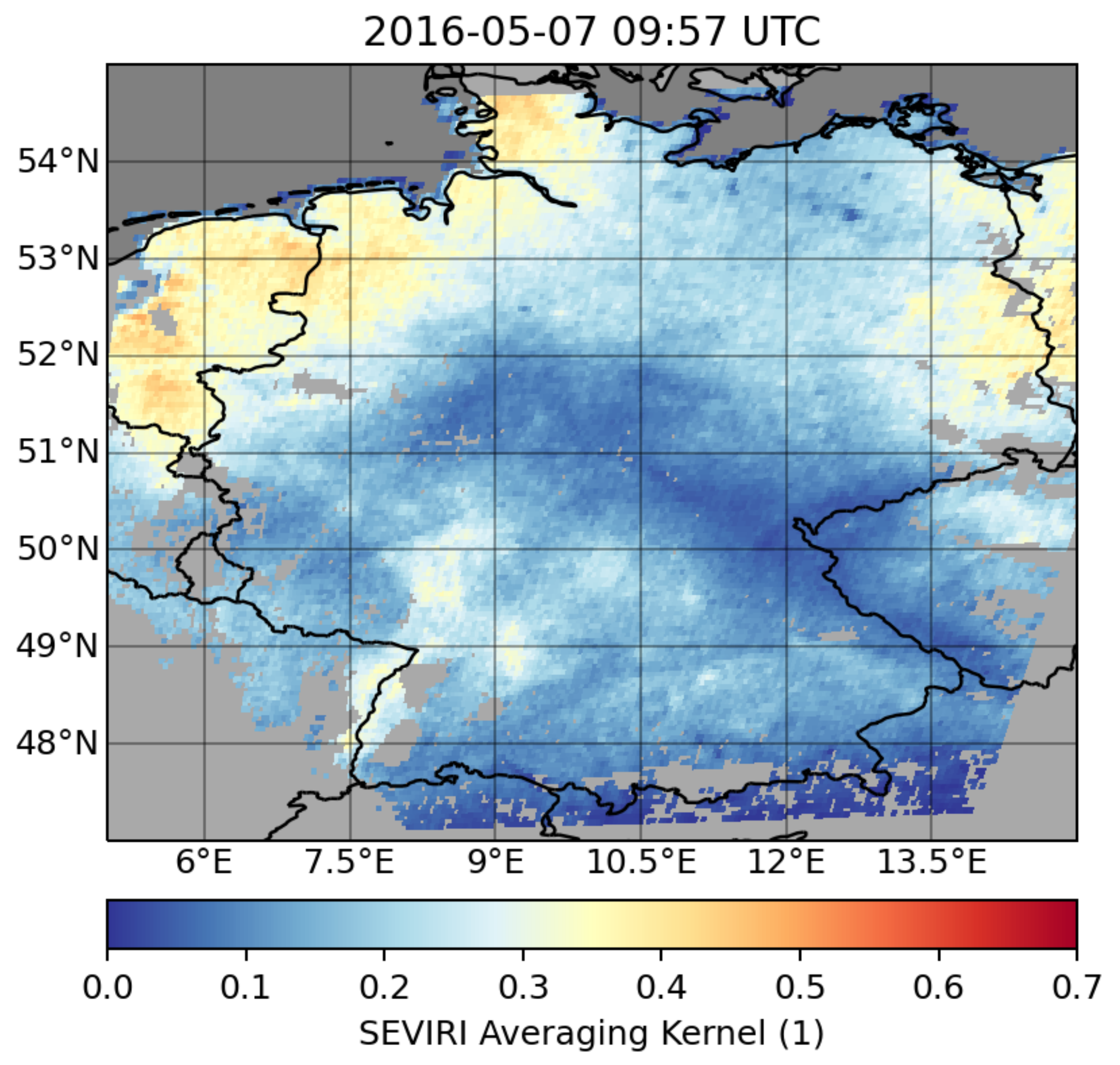
In Figure 5, SEVIRI TCWV and associated relative uncertainty over Germany on 7 May 2017 at 9:57 UTC is shown. The excerpt and plot’s design were directly adapted from [16] in correspondence with the authors. Overlaid in circles are the TCWV measurements of the GNSS Germany network available for this time step. Large scale variabilities with values ranging between 4 kg/m${}^2$ in the South and Southeast and 20 kg/m${}^2$ at the coast in the Northwest can be observed. Relative uncertainty lies in a range between 5 and 6% for lower TCWV and 6 to 8% for higher values.

Figure 6 shows TCWV retrieved from the state of the art Copernicus Sentinel-3 OLCI Water Vapour product (COWa) algorithm [16] applied to an OLCI scene on the same day at 9:51 UTC, as presented in [16]. While MSG SEVIRI has a nominal spatial resolution of 3000 m, the resolution of OLCI is 10 times higher at approx. 300 m. SEVIRI TCWV is not capable of exposing highly localised variabilities such as the stripes of high and low TCWV that can be seen in the north-eastern part of Germany in the OLCI COWa TCWV product. Patterns such as these are thought to present small-scale convective features like horizontal convective rolls [59]. The overall distribution and amounts of TCWV, however, align quite well between the two products.

3.4. Averaging Kernel for SEVIRI TCWV

The retrieved state from this OE approach can be evaluated using the Averaging Kernel (see Equation (6)). In Figure 7, the Averaging Kernels for $\partial {\widehat{x}}_{TCWV}/\partial x_{TCWV}$ show that in areas of low TCWV concentrations (<6 kg/m${}^2$), the information content is low. The difference between BT${}_{11}$ and BT${}_{12}$ is much less sensitive at low TCWV concentrations. This leads to insensitivity of the state to changes in the measurement and the algorithm is not capable of yielding much information from SEVIRI’s observations.

In other scenes (not shown) with higher TCWV values (e.g., in summer), AVKs were higher, at approx. 0.6–0.7. The median average for the 3000 scenes is 0.3.

3.5. Daily Course of SEVIRI TCWV on Semi-Clear Days

To showcase capabilities of the SEVIRI TCWV retrieval in relation to observing diurnal cycles and temporal variabilities, timeseries of days and locations where TCWV measurements from different networks were available and clear-sky conditions were prevalent throughout the day are presented.

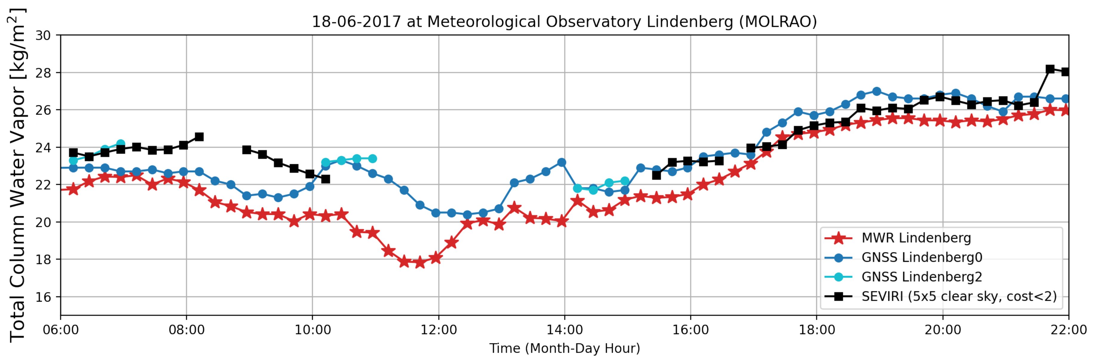
Figure 8 depicts the comparison for a case study day for 18 June 2017 at MOLRAO where MWR, and two GNSS receivers measured TCWV in parallel. AERONET measurements were not available for that specific day. Shortly after 8 a.m., high cirrus clouds pass over the site, which explains the short data gap. Between 10 a.m. and 4 p.m., retrieval of SEVIRI TCWV was disturbed or inhibited by cumulus clouds which passed over the station sporadically.

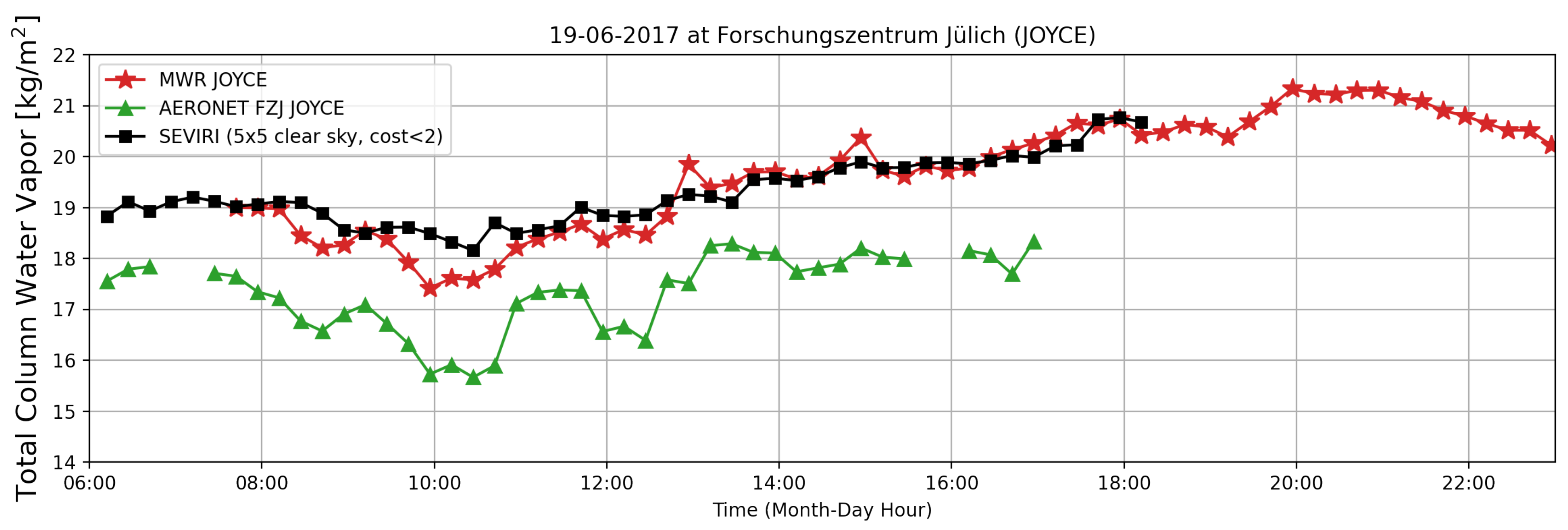
Figure 9 shows the 19 June 2017 at JOYCE. GNSS TCWV was not available on that specific day. At around 6 p.m., a wide area of clouds move over the site, which inhibit TCWV retrieval from SEVIRI.

On both days, SEVIRI TCWV follows the course of water vapour revealed by the ground-based measurements. Without going into more detail, SEVIRI TCWV seems to overestimate water vapour concentrations in the morning and becomes more accurate during the day. An investigation on the time dependency of retrieval uncertainties has not been conducted in this paper, but will be part of future work. Overall, SEVIRI TCWV stays within the uncertainties of the second ground-based observations (AERONET: 12–15% and GNSS: 1–2 kg/m${}^2$).

4. Discussion

This work presents a novel algorithm for the retrieval of TCWV from measurements in the split window bands which are primarily used for the retrieval of sea and land surface temperature. The retrieval applies an optimal estimation approach on brightness temperatures and brightness temperature differences. The forward simulation is done with the fast radiative transfer simulation RTTOV, atmospheric profiles from ERA5 reanalysis and a MODIS AQUA spectral emissivity data set.

In theory, this retrieval method can be applied to any satellite platform with an instrument that measures brightness temperatures at 11 and 12 µm. This includes current and future geostationary satellites such as GOES, HIMAWARI, FY2/4, GEO-KOMPSAT-2, Meteosat Third Generation (MTG) and instruments on-board polar-orbiting satellites such as AVHRR2/3, SLSTR, MODIS, METimage.

In this study, processing and validation is limited to the German domain and a selection of days in the year 2017. Nonetheless, since the retrieved product has a resolution of about 3.3 km × 6 km and temporal resolution of 15 min, a large number of match-ups with three well-established ground-based TCWV data sets could be collected. The validation methodology is oriented at the steps summarised in [60]. In specific, we closely followed the approach outlined in [16]. SEVIRI pixels were averaged in 5 by 5 pixels (≈16.5 km × 30 km) around each station, the next-smallest possible area (3 × 3 pixels ≈ 10 km × 18 km) did not show any significant change in the statistics.

Upon visual inspection it became clear, that retrievals with cost functions higher than 2 often included areas which are contaminated by high cirrus clouds and thus add a wet bias to the retrieved values. The comparison with AERONET TCWV with over 1275 match-ups show a wet bias of 2.85 kg/m${}^2$ and a RMSD of 3.24 kg/m${}^2$ and a high correlation coefficient at 0.97. Against the GNSS TCWV, the retrieval performed better with over 44,906 match-ups which show a low dry bias of −0.11 kg/m${}^2$ and a RMSD of 2.07 kg/m${}^2$. The small group of data points that runs offset but parallel to the 1:1 line visible in Figure 10 are match-ups with the GNSS station Besancon (BSCN), which reports substantially higher TCWV values than other surrounding GNSS stations. This discrepancy is not related with differences in the DEM, the DEM difference is at 30 m.

There were 897 match-ups with the two MWR stations for which a wet bias of 0.97 kg/m${}^2$ and RMSD of 1.63 kg/m${}^2$ were found. Since MWR TCWV is measuring in a very narrow zenith looking beam, the validation results may also be subject to small-scale fluctuations due to tropospheric turbulence. For instance, Ref. [56] observed standard deviations of 0.5 kg/m${}^2$ in MWR TCWV within 30 min time intervals.

Since the validation only covers one year and is limited to Germany, it is difficult to set the validation statistics into a context with other TCWV algorithms that were validated globally. In comparison with COWa TCWV, which was validated against the same GNSS Germany data set in [16], over the span of three years, SEVIRI TCWV compares very well. This good performance could be due to the selection of days described in Section 2.6. In [16], a bi-modal distribution is found in the scatter plots, a similar bi-modal frequency distribution can be seen in Figure 10.

The validation study on uncertainties performed against AERONET showed an overall good uncertainty calculation. Observed discrepancy and expected discrepancy agreed fairly well in the 68th and 95th percentile. However, in the 38th percentile absolute observed uncertainties were underestimated. In [16], it is argued that the relative error of AERONET TCWV with 12–15% is set too high, resulting in an overestimation in total expected discrepancy.

Figure 5 shows, that SEVIRI TCWV captures large scale variability in the water vapour field. Both COWa and the SEVIRI TCWV algorithm are sensitive to thin cirrus clouds. While thin cirrus cause an overestimation of TCWV for this SEVIRI retrieval, COWa significantly underestimates integrated water vapour in the presence of thin clouds. Both algorithms thus heavily rely on a good cloud mask. In the case of SEVIRI TCWV, the influence of thin cirrus clouds not captured by the CLAAS2 cloud mask stood out with elevated cost-functions.

In comparison to a NIR-TCWV retrieval, the smaller information content about TCWV of the TIR channels at 11 and 12 µm becomes clear. Given the fact that channel 10 (12 µm) is not directly at the wing of a water vapour absorption peak (as is the case in NIR-TCWV retrievals), but rather influenced by several smaller peaks, this is to be expected. The majority of averaging kernels lies between 0.2 and 0.5; however, especially at low TCWV (<6 kg/m${}^2$), the information content of BT${}_{11}$–BT${}_{12}$ is minimal. There, the retrieval relies on a priori TCWV, since the measurements are less sensitive. In contrast, in the NIR spectrum, the information content is high along the whole range of TCWV values, and Averaging Kernels are above 0.99 over land. Despite that, while COWa is capable of retrieving TCWV with high accuracy and high spatial resolution, SEVIRI TCWV is able to observe variations in TCWV, provided that cloud coverage is low.

In the comparison against COWa TCWV in Figure 5 and Figure 6, the lack of detail in SEVIRI TCWV stands out. However, this shortcoming is balanced out by advantages in temporal coverage: SEVIRI is able to provide clear-sky TCWV retrievals for a full disk every 15 min. As can be seen in Figure 8 and Figure 9, compared to ground-based observations, this high frequency of available TCWV estimates carry a lot of potential, e.g., the effect of approaching clouds on SEVIRI TCWV could be investigated further using liquid water path (LWP) from MWR.

5. Conclusions

The algorithm presented in this paper exploits differential water vapour absorption in the split window to improve TCWV retrievals using geostationary satellite observations. It is based on an OE retrieval, which offers a physical error characterization of retrieved TCWV. The OE’s forward operator is the fast radiative transfer model RTTOV. The retrieval is applied to MSG-SEVIRI over land surfaces in Germany. A validation study for days spread over the year 2017 against three independent ground-based TCWV data sets with stations spread over the study domain has been conducted. It concludes with absolute biases ranging between 0.11 and 2.85 kg/m${}^2$ and rmsds ranging from 1.63 to 3.24 kg/m${}^2$. This acknowledges a fair accuracy for a novel and previously untested algorithm. In an uncertainty evaluation against AERONET, the uncertainty estimates were shown to be roughly Gaussian compared to observed discrepancies. At 1, standard deviation errors aligned reasonably well. Below, at 0.5 standard deviation, uncertainties were underestimated, and above, at 2 standard deviations, uncertainties were overestimated. Averaging kernels from the OE are not as high as AVKs for NIR-TCWV retrievals. This is to be expected, in the light of lower sensitivities of BT${}_{12}$ compared to measurements at $\rho \sigma \tau$. The inclusion of further measurements could improve that. Despite that, two case studies showed that SEVIRI TCWV compares well both spatially against NIR-TCWV and temporally against ground-based TCWV.

In the future, the retrieval will be extended to the full disk and longer time periods. Then, in subsequent validation studies, further TCWV observation data sets such as MWR TCWV from the Atmospheric Radiation Measurement (ARM) network and radiosonde observations from the GCOS Upper-Air Network (GUAN) and the GCOS Reference Upper-Air Network (GRUAN) will be taken into account. Future cross-comparison on a global scale between our retrieval and approaches presented in [24,26,27] could provide valuable insight into the performance as well as advantages or disadvantages of each algorithm.

Due to the low averaging kernels and dependence on the a priori from NWP in low TCWV conditions, the application as a reference for climatological data sets is restricted. Here, we only investigate the use of the bands at 10.8 and 12 µm. However, using one or several additional channels might be beneficiary to the retrieval and increase sensitivity. We propose the investigation of a band near 13 µm. This introduces new uncertainties in the form of CO${}_2$ absorption at this wavelength, but could address the low sensitivity of the split window under dry conditions and further improve the performance across a wider range of TCWV. In [27], the PSW retrieval was extended to measurements near 6.7 µm, which proved to increase performance significantly at low TCWV. The same will be investigated for this algorithm using the MSG-SEVIRI’s 7.3 µm band.

Utilizing the differential absorption information from the NIR spectrum at the $\rho \sigma \tau$ absorption peak would drastically improve the retrieval, given the high information content there. Furthermore, the two approaches could mutually benefit from one another, since return signal over ocean (offside glint areas) in the NIR is low. On the contrary the TIR signal is much stronger over ocean and could extend existing retrieval algorithms, which work fairly over the ocean (e.g., COWa [16]). Such a configuration is already available on sensors such as MODIS or OLCI in combination with the SLSTR at a higher spatial resolution than SEVIRI. The future Flexible Combined Imager (FCI) onboard MTG, the successor of MSG, will also feature bands needed for this combined NIR-TIR approach.

In the scope of this paper, the algorithm was limited to daytime TCWV over land surfaces. Future studies will investigate the performance at night-time and over water surfaces. Over water surfaces, we expect higher accuracy due to lower variability and uncertainty in the surface emissivity.

Above all, it is obvious to extend further into the adaptation of this algorithm to other instruments and platforms. This could provide a vast amount of global, high temporally resolved TCWV observations over the time span of decades. These satellite observations could in turn be used to further study water vapour and its role in both weather and climate processes, e.g., using satellite-retrieved TCWV fields as indicators of convective initiation and improvements of (extreme) precipitation model forecasts through assimilation, as both are topics of research in the RealPEP project.