Abstract
Wildfires are natural ecological processes that generate high levels of fine particulate matter (PM2.5) that are dispersed into the atmosphere. PM2.5 could be a potential health problem due to its size. Having adequate numerical models to predict the spatial and temporal distribution of PM2.5 helps to mitigate the impact on human health. The compositional data approach is widely used in the environmental sciences and concentration analyses (parts of a whole). This numerical approach in the modelling process avoids one common statistical problem: the spurious correlation. PM2.5 is a part of the atmospheric composition. In this way, this study developed an hourly spatio-temporal PM2.5 model based on the dynamic linear modelling framework (DLM) with a compositional approach. The results of the model are extended using a Gaussian–Mattern field. The modelling of PM2.5 using a compositional approach presented adequate quality model indices (NSE = 0.82, RMSE = 0.23, and a Pearson correlation coefficient of 0.91); however, the correlation range showed a slightly lower value than the conventional/traditional approach. The proposed method could be used in spatial prediction in places without monitoring stations.
1. Introduction
Wildfires are natural or human-based phenomena that emit various air pollutants into the atmosphere [1,2]. PM2.5 is one of the most critical pollutants to human health produced by wildfires [3,4]. PM2.5, inhaled and transported by the bloodstream, can impair the lungs and other vital organs, and its impact is more harmful if the source is from wildfires [5,6]. On the other hand, PM2.5 emitted from biomass burning (carbonaceous aerosols from wildfires) contributes to one of the largest variables of uncertainty in the current estimates of radiative forcing [7,8].
The accurate predictions of fine particulate matter related to wildfires can aid decision-makers in mitigating the environmental and socio-economic impacts of wildfires [9,10,11]. In this sense, among the most important studies are those models that seek to estimate the emission of PM2.5 using a set of fixed-source profiles (land use, vegetation inventories, types of forest, chemistry, and physics characteristics) [12,13,14]. In this way, we could mention some examples, such as the BlueSky modelling framework developed by the Fire Consortium for the Advanced Modeling of Meteorology and Smoke (FCAMMS), which combines state of the art emissions, meteorology, and dispersion models to generate the best possible predictions of smoke impacts across the landscape. Another example is the Sparse Matrix Operator Kerner Emissions Modeling System (SMOKE), developed by the Center for Environmental Modeling for Policy Development (CEMPD), which is based on RatePerStart (RPS) emission rates [15]. However, the results from the emission models could be wrong even if representative source profiles are used, and thus a contradiction in the empirical evidence for ground-level monitoring could appear [16,17,18,19,20,21,22]. On the other hand, measures of PM2.5 from monitoring stations on the surface could be used in statistical models under a dispersion modelling approach. The dispersion models are usually presented in univariate spatio-temporal research [23,24,25,26]. For instance, Mirzaei et al. used a land use regression with ground-level monitoring of smoke to propose exposure models [27]. The dynamic linear modelling framework is commonly used in air quality models due to its flexibility in treating time series in both stationary and non-stationary approaches [28,29,30,31,32,33]. For instance, Cameletti et al. developed a daily spatio-temporal model for PM10 for Piemonte in Italy with an extensive network of monitoring stations [34]. Sánchez-Balseca and Pérez-Foguet, with a limited number of monitoring stations, presented hourly spatio-temporal PM2.5 modelling in wildfires events, a validation method using PM10 levels and a PM2.5/PM10 ratio was proposed as well. Both studies used DLM with a Gaussian–Mattern field due to its low computational cost [35].
PM2.5 is an air pollutant and thus part of an atmospheric composition (e.g., μg/l, mg/kg, wt%). Compositional data (CoDa) belong to a sample space called the simplex. If PM2.5 data are not treated under a compositional approach, the results could draw wrong conclusions [36,37]. One statistical problem if compositional data are not adequately treated is the spurious correlation. In a composition of two elements that sum a constant, the increase in one of them means reducing the other component, and vice versa. The two elements have an inverse correlation imposed upon them, even if these two elements have no relationship. This imposed correlation is called a spurious correlation and could be eliminated through transformations in the form of logarithms of ratios (log-ratios) [38]. The isometric log-ratio (ilr) transformation is the most used due to its advantage of representing the simplex space orthogonally [39]. In addition, the CoDa approach has been widely used in other environmental fields (soil, water, geology, etc.), but the application in air pollution modelling is scarce.
This article presented a compositional, hourly spatio-temporal model for PM2.5 based on a dynamic linear modelling framework. To extend the results of the model in places with no monitoring stations, a Gaussian–Mattern field is used. The remainder of this article provides the site description, datasets used, a brief background on the statistical tools (DLM and CoDa), the methodology (Section 2), the results (Section 3), the discussion (Section 4), and the principal conclusions (Section 5).
2. Data and Methodology
2.1. Wildfire Description
Quito had unprecedented wildfires in September 2015, and the 14th of September was the most remarkable air pollution event. Quito is located in Ecuador in the Andean mountains at 2800 m.a.s.l., and it has 2,240,000 inhabitants. Figure 1 presents the satellite image that represents the wildfire event with points of red colour. The MODIS Terra/Aqua sensor platform was used to obtain the thermal anomalies/active fire image [40]. The yellow points are the monitoring stations for PM2.5.
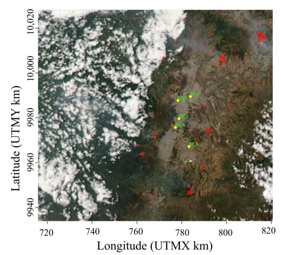
Figure 1.
Wildfire event on 14 September 2015, obtained from the MODIS-Terra/Aqua sensor platform in Quito. The wildfires are represented by red points, and the monitoring stations by yellow points.
2.2. Data
2.2.1. PM2.5 Data
PM2.5 data were collected hourly during September (720 hours) by the Air Quality Network of Quito, which is formed by five monitoring stations, and they are described in Table 1. The monitoring network used a Thermo Fisher Scientific FH62C14-DHS Continuous Ambient Particulate Monitor 5014i with beta rays’ attenuation method (Waltham, Massachusetts, USA), as suggested by the Environmental Protection Agency (EPA). The Air Quality Network of Quito is a permanent air pollution surveillance network. The data were obtained from the open-source online data repository managed by the environmental agency of Quito, and hosted at Secretaria de Ambiente del Distrito Metropolitano de Quito [41].

Table 1.
Monitoring stations for PM2.5 and their main characteristics.
2.2.2. Meteorological Data
The meteorological data were collected from meteorological assimilation systems based on satellite data. This article used Modern-Era Retrospective analysis for Research and Applications version 1 and 2 (MERRA and MERRA-2) from NASA’s Giovanni web platform; MERRA-2 published many analysis products used in meteorological and air quality modelling [42,43]. Some works used the soil surface temperature variable to indicate wildfire events [44,45,46]. Table 2 shows the main characteristics of meteorological data.
Table 2.
Meteorological data descriptions.
2.3. Statistical Modelling
2.3.1. Dynamic Linear Models (DLM)
Two equations defined the dynamic linear modelling; the first one is denoted as the observation equation. The dependent variable, , is the observed generic pollutant concentration at spatial location (on time ( and it is described in Equation (1):
where denotes the measurement error, which is assumed to be independent, and it has a variance, . The vector of regression coefficients is represented by vector represents a vector of regressors that change temporally. Operator “×” is used to indicate multiplication of scalars, vectors or matrices depending on the context in this article. The second equation that describes the dynamic linear modelling is related to the term ; its name is the system equation, and it describes a dynamic autoregressive first-order model, shown as:
where is the temporal and spatial error; it has a normal distribution and a variance, . The temporal and spatial variance ( is based on the correlation between monitoring stations and their Euclidean spatial distance using a Gaussian–Mattern field, and is parameterized by the empirically derived correlation range (ρ). This empirically derived correlation range is the distance at which the correlation is close to 0.1. For more details, see [34,47,48,49].
2.3.2. Compositional Data (CoDa) Approach
Compositional data belong to a sample space called the simplex SD, which could be represented in mathematical terms as:
where K is defined a priori and is a positive constant. represents the components of a composition. The next equation represents the isometric log-ratio (ilr) transformation (Egozcue et al. [36]).
where is the vector with D components of the compositions, is a matrix that denotes the orthonormal basis in the simplex, and is the vector with the log-ratio coordinates of the composition on the basis, . The ilr transformation allows for the definition of the orthonormal coordinates through the sequential binary partition (SBP), and thus, the elements of , with respect to the , could be obtained using Equation (5) (for more details see [39]).
where and are the geometric means of the components in the kth partition, and and are the number of components. After the log-ratio coordinates are obtained, conventional statistical tools can be applied. For a 2-part composition, , an orthonormal basis could be = [], and then the log-ratio coordinate is defined using Equation (6):
After the log-ratio coordinates are obtained, conventional statistical tools can be applied.
2.4. Methodology: Proposed Approach Application in Steps
To propose a compositional spatio-temporal PM2.5 model in wildfire events, our approach encompasses the following steps: (i) pre-processing data (PM2.5 data expressed as hourly 2-part compositions), (ii) transforming the compositions into log-ratio coordinates, (iii) applying the DLM to compositional data, and (iv) evaluating the compositional spatio-temporal PM2.5 model.
Models were performed using the INLA [48], OpenAir, and Compositions [50] packages in the R statistical environment, following the algorithm showed in Figure 2. The R script is described in [51].
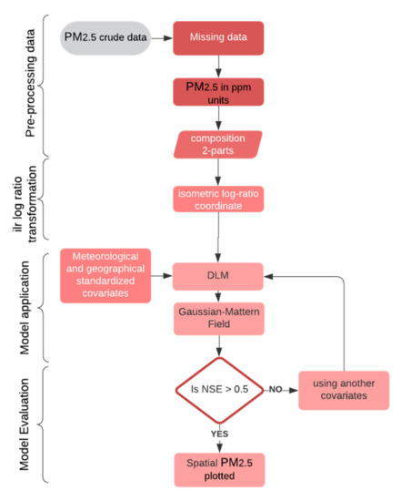
Figure 2.
Algorithm of spatio-temporal PM2.5 model in wildfire events using DLM.
Step 1. Pre-processing data
To account for missing daily PM2.5 data, we used the compositional robust imputation method of k-nearest neighbor imputation [52,53]. Then, the air density from the ideal gas law was used to transform the concentration from volume to weight (Equation (7)). The concentration by weight has absolute units, while the volume concentration has relative units that depend on the temperature [49]. The air density is defined by temperature (T), pressure (P), and the ideal gas constant for dry air (R).
The closed composition can then be defined as , where Res is the residual or complementary part. We fixed K = 1 million (ppm by weight). Due to the sum() for all compositions x is less than K, and the complementary part is Res = K - sum() for each hour. The meteorological and geographical covariates were standardized using both the mean and standard deviation values of each covariate. For meteorological missing data, a simple imputation method was used.
Step 2. Log-ratio transformation
The two components (PM2.5 and the residual) are first log-transformed into one log-ratio coordinate for each hour () using Equation (6), where represents the PM2.5 levels and describes the residual part (Res) for each hour.
Step 3. Model application
The log-ratio coordinate is the dependent variable () in the DLM modelling framework, and the independent variables () are described by the meteorological data that change spatial-temporally. The posterior estimates—, , , , , and ρ—are obtained from the regression using Bayesian inference. The empirically derived correlation range was defined in km. The spatial distribution of PM2.5 in places with no monitoring stations was featured using a triangular irregular mesh for monitoring stations of PM2.5 and a grid of 4 km between each intersection of meteorological data, as proposed by Sánchez-Balseca and Pérez-Foguet (2020) [49].
It is necessary to recover the original units for the estimates in compositional data analysis [54]. Once results are back-transformed in proportions, (pE; sum(pE) = 1), they are multiplied by K to obtain the model results in original units.
Step 4. Model Evaluation
For this step, the Nash–Sutcliffe efficiency index (NSE) and the Pearson correlation coefficient were used. Both the NSE and the Pearson correlation are independent of the scale of measurement of the variables. The NSE scale ranges from 0 to 1, whereby NSE = 1 means the model is perfect, NSE = 0 means that the model is equal to the average of the observed data, and negative values mean that the average is a better predictor.
3. Results
The compositional spatio-temporal air pollution modelling used five monitoring stations and 720 hours in a wildfire event. The posterior estimates (mean, quantiles, and standard deviation) for the parameters , , a, and ρ are presented in Table 3. The spatial variance ( was slightly more significant than the measure variance (). The empirically derived correlation range was about 26.006 km; this represents the distance at which the correlation is close to 0.1. The parameter is 0.7547, which was directly proportional to the spatial and temporal variance.
Table 3.
Posterior estimates (mean, standard deviation, and quantiles).
The compositional model presented an intercept of about −12.618 that represents, in the original units, 0.018 ppm of PM2.5 (see Table 4). Considering the threshold for fine particulate matter suggested by WHO in a 24 h average, about 0.022 ppm (using an air density value equal to 1.15 kg/m3 to transform it into concentration in mass), the intercept value does not exceed the limit in a wildfire event. The regression coefficients of altitude, air temperature, and radiation had negative values. The concentration of PM2.5 decreases with increasing altitude [55]. The air temperature and radiation are related to thermal inversion and air density, and thus their increase means the PM2.5 concentration decreases [56]. The surface soil temperature had a positive influence on the concentration of PM2.5.
Table 4.
Regression coefficients of meteorological and geographical covariates.
The compositional model presented an NSE of 0.82, an RMSE of 0.23, and a Pearson correlation coefficient of 0.91. Figure 3 shows the highest hourly concentration of PM2.5 presented in the wildfire at 16:00 h on 14 September 2015. It illustrates the spatial il-coordinate (without back-transformed process) and the logarithmic concentration of PM2.5 on its original units (ppm).
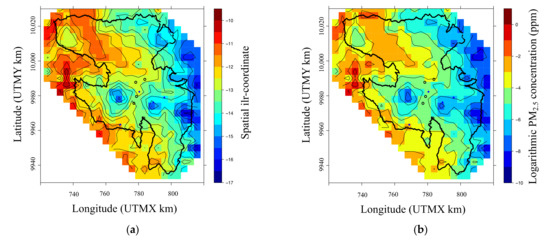
Figure 3.
(a) The predictive ilr-coordinate related to PM2.5 concentration on 14 September 2015; (b) the predictive logarithmic concentration of PM2.5 in ppm on 14 September 2015. The black border shows the administrative boundary of Quito.
4. Discussion
This article presented a compositional spatio-temporal air pollution model for PM2.5 using meteorological and geographical covariates. The proposed model showed adequate quality model metrics; in addition, spurious correlation was avoided by applying the ilr-transformation. The values of the quality model metrics obtained in this article were similar to those obtained using a conventional approach. The RMSE criterion displayed the most evident difference; it was about 0.23 when using a compositional process, whereas it was about 0.32 when using a traditional approach. The empirically derived correlation range, when using a conventional approach, was about 27 km; this is slightly higher than the value obtained in previous work, which was 26 km (Sánchez-Balseca and Pérez-Foguet [35]). In this sense, the compositional approach had better quantitative modelling performance but a slightly lower capacity for spatial correlation than the conventional approach [34].
The interpretation for modelling ilr-coordinates could be complicated because the information is only in the relationships between the parts [36]. For this reason, the log-ratio used in this article should be interpreted as the influence of PM2.5 in the composition of air when using a relative approach. This approach transforms a univariate analysis into a bivariate (multivariate) analysis [37]. Usually, the variable thermal anomalies are used to identify wildfires; however, this information is available only two times per day in some territories. For this reason, this article uses the temperature of the surface soil as a spatial wildfire indicator due to the temporal resolution needed (hourly). However, the PM2.5 measures could be distorted by the secondary organic aerosol (SOA) formation [57,58,59].
For further works, the compositional approach for univariate analysis could be performed using the centered log-ratio (clr) or the additive log-ratio (alr), which Aitchison proposed in 1982 [60].
5. Conclusions
The compositional approach performs the modelling of PM2.5 slightly better than the conventional approach. However, the compositional approach presented a slightly lower correlation range than the traditional approach. The compositional spatio-temporal PM2.5 model showed adequate quality indexes and thus could be used to determine the concentration of fine particulate matter in places where there are no monitoring stations for wildfire scenarios. This information could allow for the determination of zones with significant impacts on human health.
Author Contributions
Conceptualization, J.S.-B. and A.P.-F.; methodology, J.S.-B.; software, J.S.-B.; validation, A.P.-F.; formal analysis, J.S.-B.; investigation, J.S.-B.; data curation, J.S.-B.; writing—original draft preparation, J.S.-B.; writing—review and editing, A.P.-F.; supervision, A.P.-F. All authors have read and agreed to the published version of the manuscript.
Funding
This research received no external funding.
Institutional Review Board Statement
Not applicable.
Informed Consent Statement
Not applicable.
Data Availability Statement
R script and Dataset are available in https://zenodo.org/record/5532476#.YVg2qS1t-9Y, accessed on 19 August 2021.
Acknowledgments
Joseph Sánchez Balseca is the recipient of a full scholarship from the Secretaria de Educación Superior, Ciencia, Tecnología e Innovación (SENESCYT), Ecuador. We thank the research group on Engineering Sciences and Global Development (EScGD) and the Agència de Gestió d’Ajuts Universitaris i de Recerca de la Generalitat de Catalunya (Ref. 2017 SGR 1496).
Conflicts of Interest
The authors declare no conflict of interest.
References
- Fillippi, J.-B.; Bosseur, F.; MAri, C.; Lac, C. Simulation of a Large Wildfire in a Coupled Fire-Atmosphere Model. Atmosphere 2018, 9, 218. [Google Scholar] [CrossRef]
- Navarro, K.; Schweizer, D.; Balmes, J.; Cisneros, R. A Review of Community Smoke Exposure from Wildfire Compared to Prescribed Fire in the United States. Atmosphere 2018, 9, 185. [Google Scholar] [CrossRef]
- Castagna, J.; Senatore, A.; Bencardino, M. Concurrent Influence of Different Natural Sources on the Particulate Matter in the Central Mediterranean Region during a Wildfire Season. Atmosphere 2021, 12, 144. [Google Scholar] [CrossRef]
- Jiménez, P.; Muñoz-Esparza, D.; Kosović, B. Minimize the Impacts of Wildland Fires: Applications to the Chimney Tops II Wildland Event. Atmosphere 2018, 9, 197. [Google Scholar] [CrossRef]
- Aguilera, R.; Corringham, T.; Gershunov, A.; Benmarhnia, T. Wildfire smoke impacts respiratory health more than fine particles form other sources: Observational evidence from Southern California. Nat. Commun. 2021, 12, 1493. [Google Scholar] [CrossRef] [PubMed]
- Franzi, L.; Bratt, J.; Williams, K.; Last, J. Why is particulate matter produced by wildfires toxic to lung macrophages? Toxicol. Appl. Pharmacol. 2011, 257, 182–188. [Google Scholar] [CrossRef]
- Chakrabarty, R.; Beres, N.; Moosmüller, H.; China, S.; Mazzoleni, C.; Dubey, M.; Liu, L.; Mishchenko, M. Soot superaggregates from flaming wildfires and their direct radiative forcing. Sci. Rep. 2014, 4, 5508. [Google Scholar] [CrossRef]
- Mallia, D.; Kochanski, A.; Urbanski, S.; Lin, J. Optimizing Smoke and Plume Rise Modeling Approaches at Local Scales. Atmosphere 2018, 9, 166. [Google Scholar] [CrossRef]
- Malik, A.; Rajam, M.; Puppala, N.; Koouri, P.; Kumar, V.; Liu, Q.; Gao, J. Data-Driven Wildfire Risk Prediction in Northern California. Atmosphere 2021, 12, 109. [Google Scholar] [CrossRef]
- Martínez, J.; Vega-Garcia, C.; Chuvieco, E. Human-caused wildfire risk rating for prevention planning in Spain. J. Environ. Manag. 2009, 90, 1241–1252. [Google Scholar] [CrossRef]
- Nunes, A.; Lourenç, L.; Castro-Meira, A. Exploring spatial patterns and drivers of forest fires in Portugal (1980–2014). Sci. Total. Environ. 2016, 573, 1190–1202. [Google Scholar] [CrossRef]
- Hodzic, A.; Madronich, S.; Bohn, B.; Massie, S.; Menut, L.; Wiedinmyer, C. Wildfire particulate matter in Europe during summer 2003: Meso-scale modeling of smoke emissions, transport and radiative effects. Atmos. Chem. Phys. 2007, 7, 4043–4064. [Google Scholar] [CrossRef]
- Koplitz, S.; Nolte, C.; Pouliot, G.; Vukovich, J.; Beidlerc, J. Influence of uncertainties in burned area estimates on modeled wildland fire PM2.5 and ozone pollution in the contiguous U.S. Atmos. Environ. 2018, 191, 328–339. [Google Scholar] [CrossRef] [PubMed]
- Martins, V.; Miranda, A.; Carvalho, A.; Schaap, M.; Borrego, C.; Saá, E. Impact of forest fires on particulate matter and ozone levels during the 2003, 2004 and 2005 fire seasons in Portugal. Sci. Total. Environ. 2012, 414, 53–62. [Google Scholar] [CrossRef] [PubMed]
- Baek, B.H.; Seppanen, C. CEMPD/SMOKE: SMOKE v4.8.1 Public Release. Zenodo. 2021. Available online: https://zenodo.org/record/4480334#.YVhEhC1t-9Y (accessed on 15 September 2021). [CrossRef]
- Lee, S.; Kim, H.; Yan, B.; Cobb, C.; Hennigan, C.; Nichols, S.; Russell, A. Diagnosis of Aged Prescribed Burning Plumes Impacting an Urban Area. Environ. Sci. Technol. 2008, 42, 1438–1444. [Google Scholar] [CrossRef] [PubMed]
- Majdi, M.; Turquety, S.; Sartelet, K.; Legorgeu, C.; Menut, L.; Kim, Y. Impact of wildfires on particulate matter in the Euro-Mediterranean in 2007: Sensitivity to some parameterizations of emissions in air quality models. Atmos. Chem. Phys. 2019, 19, 785–812. [Google Scholar] [CrossRef]
- Richardson, C.; Rutherford, S.; Agranovski, I. Characterization of particulate emissions from Australian open-cut coal mines: Toward improved emission estimates. J. Air Waste Manag. Assoc. 2018, 68, 598–607. [Google Scholar] [CrossRef]
- Wang, X.; Watson, J.; Chow, J.; Gronstal, S.; Kohl, S. An Efficient Multipollutant System for Measuring Real-World Emissions from Stationary and Mobile Sources. Aerosol Air Qual. Res. 2012, 12, 145–160. [Google Scholar] [CrossRef]
- Watson, J.; Chow, J.; Lowenthal, D.; Chen, A.; Shaw, S.; Edgerton, E.; Blanchard, C. PM2.5 source apportionment with organic markers in the Southeastern Aerosol Research and Characterization (SEARCH) study. J. Air Waste Manag. Assoc. 2015, 65, 1104–1118. [Google Scholar] [CrossRef]
- Wiedinmyera, C.; Quayleb, B.; Geronc, C.; Belotea, A.; McKenzied, D.; Zhange, X.; Klos, K. Estimating emissions from fires in North America for air quality modeling. Atmos. Environ. 2006, 40, 3419–3432. [Google Scholar] [CrossRef]
- Ying, Q.; Feng, M.; Song, D.; Wu, L.; Hu, J.; Zhang, H.; Li, X. Improve regional distribution and source apportionment of PM2.5 trace elements in China using inventory-observation constrained emission factors. Sci. Total. Environ. 2018, 624, 355–365. [Google Scholar] [CrossRef] [PubMed]
- Arakia, S.; Shima, M.; Yamamoto, K. Spatiotemporal land use random forest model for estimating metropolitan NO2 exposure in Japan. Sci. Total. Environ. 2018, 634, 1269–1277. [Google Scholar] [CrossRef]
- He, J.; Ding, S.; Liu, D. Exploring the spatiotemporal pattern of PM2.5 distribution and its determinants in Chinese cities based on a multilevel analysis approach. Sci. Total. Environ. 2019, 659, 1513–1525. [Google Scholar] [CrossRef] [PubMed]
- Hu, H.; Hu, Z.; Zhong, K.; Xu, J.; Zhang, F.; Zhao, Y.; Wu, P. Satellite-based high-resolution mapping of ground-level PM2.5 concentrations over East China using a spatiotemporal regression kriging model. Sci. Total. Environ. 2019, 672, 479–490. [Google Scholar] [CrossRef] [PubMed]
- Pak, U.; Ma, J.; Ryu, U.; Ryom, K.; Juhyoke, U.; Pak, K.; Pak, C. Deep learning-based PM2.5 prediction considering the spatiotemporal correlations: A case study of Beijing, China. Sci. Total. Environ. 2020, 699, 133561. [Google Scholar] [CrossRef]
- Mirzaei, M.; Bertazzon, S.; Couloigner, I. Modeling Wildfire Smoke Pollution by Integrating Land Use Regression and Remote Sensing Data: Regional Multi-Temporal Estimates for Public Health and Exposure Models. Atmosphere 2018, 9, 335. [Google Scholar] [CrossRef]
- Cameletti, M.; Ignaccolo, R.; Bande, S. Comparing spatio-temporal models for particulate matter in Piemonte. Environmetrics 2011, 22, 985–996. [Google Scholar] [CrossRef]
- Cocchi, D.; Greco, F.; Trivisano, C. Hierarchical space-time modelling of PM10 pollution. Atmos. Environ. 2007, 41, 532–542. [Google Scholar] [CrossRef]
- Fassò, A.; Finazzi, F. Maximum likelihood estimation of the dynamic coregionalization model with heterotopic data. Environmentrics 2011, 22, 735–748. [Google Scholar] [CrossRef]
- Sahu, S. Handbook of Statistics—Hierarchical Bayesian Models for Space–Time Air Pollution Data; Elsevier: Southampton, UK, 2012. [Google Scholar]
- Shaddick, G.; Thomas, M.L.; Jobling, A.; Brauer, M.; Donkelaar, A.V.; Burnett, R.; Prüss-Ustün, A. Data integration model for air quality: A hierarchical approach to the global estimation of exposures to ambient air pollution. R. Stat. Soc. 2018, 67, 231–253. [Google Scholar] [CrossRef]
- Tonellato, S. A multivariate time series model for the analysis and prediction of carbon monoxide atmospheric concentrations. J. R. Stat. Soc. Ser. C Appl. Stat. 2001, 50, 187–200. [Google Scholar] [CrossRef]
- Cameletti, M.; Lindgren, F.; Simpson, D.; Rue, H. Spatio-temporal modeling of particulate matter concentration through the SPDE approach. AStA Adv. Stat. Anal. 2013, 97, 109–131. [Google Scholar] [CrossRef]
- Sánchez-Balseca, J.; Pérez-Foguet, A. Modelling hourly spatio-temporal PM2.5 concentration in wildfire scenarios using dynamic linear models. Atmos. Res. 2020, 242, 104999. [Google Scholar] [CrossRef]
- Egozcue, J.; Daunis-i-Estadella, J.; Pawlowsky-Glahn, V.; Hron, K.; Filzmoser, P. Simplicial regression. The normal model. J. Appl. Probab. Stat. 2012, 6, 87–108. [Google Scholar]
- Filzmoser, P.; Hron, K.; Reimann, C. The bivariate statistical analysis of environmental (compositional) data. Sci. Total. Environ. 2010, 408, 4230–4238. [Google Scholar] [CrossRef] [PubMed]
- Buccianti, A.; Mateu, G.; Pawlowsky, V. Compositional Data Analysis in the Geosciences; Geological Society: London, UK, 2006. [Google Scholar]
- Egozcue, J.; Pawlowsky-Glahn, V. Groups of parts and their balances in compositional data analysis. Math. Geol. 2005, 37, 795–828. [Google Scholar] [CrossRef]
- Giglio, L.; Justice, C. MOD14A2 MODIS/Terra Thermal Anomalies/Fire 8-Day L3 Global 1km SIN Grid V006. NASA EOSDIS Land Processes DAAC. 2015. Available online: https://lpdaac.usgs.gov/products/mod14a2v006/ (accessed on 15 September 2019). [CrossRef]
- Secretaria de Ambiente del DMQ. Reporte de Calidad de l Aire, Especies Medidas. 2015. Available online: http://190.11.24.212/reportes/ReporteHorariosData.aspx (accessed on 15 September 2018).
- Kuo, C.-L. Assessments of Ali, Dome A, and Summit Camp for mm-wave Observations Using MERRA-2 Reanalysis. Astrophys. J. 2017, 848, 64. [Google Scholar] [CrossRef]
- Qin, W.; Zhang, Y.; Chen, J.; Yu, Q.; Cheng, S.; Li, W.; Tian, H. Variation, sources and historical trend of black carbon in Beijing, China based on ground observation and MERRA-2 reanalysis data. Environ. Pollut. 2018, 245, 853–863. [Google Scholar] [CrossRef] [PubMed]
- Bailey, A.; Murray, A. Fire Temperatures in Grass, shrub and Aspen Forest Communities of Central Alberta. J. Range Manag. 1980, 33, 37–40. [Google Scholar] [CrossRef]
- Jolly, M.; Cochrane, M.; Freeborn, P.; Holden, Z.; Brown, T.; Williamson, G.; Bowman, D. Climate-induced variations in global wildfire danger from 1979 to 2013. Nat. Commun. 2015, 6, 7537. [Google Scholar] [CrossRef]
- Liu, J.; Weng, F.; Li, Z.; Cribb, M. Hourly PM2.5 Estimates from a Geostationary Satellite Based on an Ensemble Learning Algorithm and Their Spatiotemporal Patterns over Central East China. Remote Sens. 2019, 11, 2120. [Google Scholar] [CrossRef]
- Cressie, N. Statistics for Spatial Data, Revised Edition; John Wiley & Sons: Michigan, MI, USA, 1993. [Google Scholar]
- Lindgren, F.; Rue, H. Bayesian Spatial Modelling with R-INLA. J. Stat. Softw. 2015, 63, 1–25. [Google Scholar] [CrossRef]
- Sánchez-Balseca, J.; Pérez-Foguet, A. Spatio-temporal air pollution modelling using a compositional approach. Heliyon 2020, 6, e04794. [Google Scholar] [CrossRef] [PubMed]
- Van den Boogaart, K.G.; Tolosana-Delgado, R.; Bren, M. Compositions: Compositional Data Analysis. R Package Versión 1.40-2. 2018. Available online: https://cran.r-project.org/web/packages/compositions (accessed on 20 December 2018).
- Sánchez-Balseca, J.; Pérez-Foguet, A. Compositional Spatio-Temporal PM2.5 Modelling in Wildfires (R Script and Dataset) (V1.0) [Data set]. Zenodo. 2021. Available online: https://zenodo.org/record/5532476#.YVhE7y1t9AY (accessed on 27 September 2021). [CrossRef]
- Hron, K.; Templ, M.; Filzmoser, P. Imputation of Compositional Data Using Robust Methods. Department of Statistics and Probability Theory, Vienna University of Technology; Vienna University of Technology: Vienna, Austria, 2008. [Google Scholar]
- Martín-Fernández, J.; Barceló-Vidal, C.; Pawloswsky-Glahn, V. Dealing with zeros and missing values in compositional data sets using nonpara- metric imputation. Math. Geol. 2003, 35, 253–278. [Google Scholar] [CrossRef]
- Martín-Fernandez, J.A.; Raju, N.J.; Egozcue, J.J.; Pawlowsky-Glahn, V.; Olea, R.A. How to recover the original units for the estimates in compositional data analysis? In Proceedings of the 8th International Workshop on Compositional Data Analysis, CODAWORK, Terrassa, Spain, 3–8 June 2019. [Google Scholar]
- Si-Jia, L.; Dongsheng, W.; Xiao-Bing, L.; Zhanyong, W.; Ya, G.; Zhong-Ren, P. Three-dimensional distribution of fine particulate matter concentrations and synchronous meteorological data measured by an unmanned aerial vehicle (UAV) in Yangtze River Delta, China. Atmos. Meas. Technol. 2016, 1–19. [Google Scholar] [CrossRef]
- Hasheminassab, S.; Pakbin, P.; Delfino, R.; Schauer, J.; Sioutas, C. Diurnal and seasonal trends in the apparent density of ambient fine and coarse particles in Los Angeles. Environ. Pollut. 2014, 187, 19–26. [Google Scholar] [CrossRef] [PubMed][Green Version]
- Price, D.J.; Kacarab, M.; Cocker, D.R.; Purvis-Roberts, K.L.; Silva, P. Effects of temperature on the formation of secondary organic aerosol from amine precursors. Aerosol Sci. Technol. 2016, 50, 1216–1226. [Google Scholar] [CrossRef]
- Soleimanian, E.; Mousavi, A.; Taghvaee, S.; Sowlat, M.; Hasheminassab, S.; Polidori, A.; Sioutas, C. Spatial trends and sources of PM2.5 organic carbon volatility fractions (OCx) across the Los Angeles Basin. Atmos. Environ. 2019, 209, 201–211. [Google Scholar] [CrossRef]
- Takekawa, H.; Minoura, H.; Yamazaki, S. Temperature dependence of secondary organic aerosol formation by photo-oxidation of hydrocarbons. Atmos. Env. 2003, 37, 3413–3424. [Google Scholar] [CrossRef]
- Aitchison, J. The statistical analysis of compositional data (with discussion). J. R. Stat. Soc. 1982, 44, 139–177. [Google Scholar] [CrossRef]


Publisher’s Note: MDPI stays neutral with regard to jurisdictional claims in published maps and institutional affiliations. |
© 2021 by the authors. Licensee MDPI, Basel, Switzerland. This article is an open access article distributed under the terms and conditions of the Creative Commons Attribution (CC BY) license (https://creativecommons.org/licenses/by/4.0/).