Comparison of Top-Down and Bottom-Up Road Transport Emissions through High-Resolution Air Quality Modeling in a City of Complex Orography

Abstract

Vehicular emissions are a predominant source of pollution in urban environments. However, inherent complexities of vehicular behavior are sources of uncertainties in emission inventories (EIs). We compare bottom-up and top-down approaches for estimating road transport EIs in Manizales, Colombia. The EIs were estimated using a COPERT model, and results from both approaches were also compared with the official top-down EI (estimated from IVE methodology). The transportation model PTV-VISUM was used for obtaining specific activity information (traffic volumes, vehicular speed) in bottom-up estimation. Results from COPERT showed lower emissions from the top-down approach than from the bottom-up approach, mainly for NMVOC (−28%), PM₁₀ (−26%), and CO (−23%). Comparisons showed that COPERT estimated lower emissions than IVE, with higher differences than 40% for species such as PM₁₀, NO_X, and CH₄. Furthermore, the WRF–Chem model was used to test the sensitivity of CO, O₃, PM₁₀, and PM_2.5 predictions to the different EIs evaluated. All studied pollutants exhibited a strong sensitivity to the emission factors implemented in EIs. The COPERT/top-down was the EI that produced more significant errors. This work shows the importance of performing bottom-up EI to reduce the uncertainty regarding top-down activity data.

1. Introduction

The transport sector is one of the primary sources of pollutants in urban centers due to the accelerated and sustained increase in motorization rates [1,2]. Emissions from road transport are commonly estimated through atmospheric emission inventories (EIs). These are the starting point for evaluating and implementing air quality management plans (AQMP), which include chemical transport models for atmospheric pollutants [3,4].

Estimating emissions from road transport is a complex process that relates information on air pollutant emission rates according to the operating conditions of the vehicle fleet, called emission factors (g/veh-km), and data on vehicle activity (e.g., distance traveled by vehicles, vehicle technology, and operating conditions). Consequently, the quality of EIs depends on the reliability of both the activity data and the emission factors (EF) [5,6].

In Latin America, few cities have measured EF in the field. Some examples are Santiago (Chile), Sao Paulo (Brazil), and Londrina (Brazil) [7,8,9] which have measured EF adjusted to traffic conditions and vehicle fleet. The road transport EIs developed in Colombia use international emission models, mainly from the United States or Europe. Models such as COPERT, MOVES, or IVE in their different versions have been used completely (emission estimation) or partially (use of emission factors) to establish EI [2,10,11,12]. The models differ mainly in the type and amount of input data, the estimated pollutants, the available vehicle technologies, and the type of correction and adjustment of the EF.

Depending on the availability of information and the level of detail required, the model is selected, and the EI is carried out following the approach: top-down (aggregated activity information) or bottom-up (specific activity information). The selection of the approach does not determine its correct implementation [3,13], and, in both cases, the inherent complexities of vehicular behavior in urban areas are a source of significant uncertainties in EI. However, a top-down approach where vehicle activity data are aggregated and all-day traffic conditions are not represented at the link level (flows and speeds) could affect the resulting emissions [5]. On the other hand, the bottom-up approach could improve the representation of the calculated vehicular emissions, since detailed information is obtained (through transport models) about the spatial distribution of types of roads and activity information of the vehicles, such as the average speed along road corridors and its temporal distribution [5,14,15].

Although EIs are essential tools in air quality management, they only provide information at a specific time and place without identifying the relationship with the observed data (ambient air measurements) [16,17]. In this sense, air quality modeling allows studying and forecasting the dynamics of ambient air, including the analysis of emission sources (EIs disaggregated spatially and temporally), meteorological processes, and physical and chemical processes [18,19,20]. Eulerian chemical transport models (CTM) are powerful tools for air quality studies at an urban or regional scale [18,19]. Therefore, air quality modeling turns out to be useful as a validation tool for EIs and to corroborate the reliability of activity data and emission factors, by comparing the results with observations (ambient air measurements). Modeling is also a fundamental tool in management plans. Some studies have integrated different tools for the assessment of air quality such as EI, transport models, and air quality models [5,18,19,20,21,22,23,24].

The city of Manizales, Colombia is an intermediate city with an urban population of 405,234 inhabitants in 2018 (93% lived in the urban area); its urban area is approximately 54 km² [25]. The city is located at 2150 m.a.s.l. and is characterized by high annual precipitation (1670 mm), daily temperatures between 12 and 24 °C, and low wind speeds (<4 m/s). The city is close to the Nevado del Ruiz volcano (approximately 28 km away to the southeast), which has registered significant activity since 2010 [26]. The circulation patterns in the city are dominated by mountain–valley wind oscillations [19,27]. Manizales has two EIs in different years that include road transport using the IVE model [28,29]. The last EI performed with the IVE model in the city revealed that emissions are dominated by on-road mobile sources (vehicular fleet of 169,142 vehicles), representing more than 80% of the emissions of all criteria pollutants, except for SO₂ (emitted mainly by stationary sources). These previous exercises have applied top-down approaches for estimating vehicular emission fluxes in their local EI; however, they have highlighted the importance of using a bottom-up approach in order to have a specific representation of changes in vehicle activity in space and time [28,29]. Furthermore, the application of the IVE model presents limitations for future estimates of the EI because it has not received updates in the base EF since 2008. Consequently, the IVE model has no EF available for new vehicle technologies greater than Euro 5 entering Colombia, i.e., EF are available for private vehicles only up to Euro IV and for buses only up to Euro V with gasoline and diesel as fuels [30]. In contrast, the application of the COPERT model has increased [5,31] because it has been constantly updated (last update in 2021) and directly related to the inclusion of EF for new vehicle technologies [32].

The objective of this work was to evaluate top-down and bottom-up estimates of the road transport emissions inventory for the city of Manizales (base year 2017) using emissions comparison and high-resolution air quality modeling. The COPERT model was applied to estimate EF adjusted to local conditions. On the one hand, the bottom-up approach estimation was developed with the transportation model developed in PTV-VISUM to obtain specific activity information (traffic volumes, vehicular speed) of the vehicle fleet. On the other hand, the top-down approach using the COPERT 5.4 software (Emisia, Thessaloniki, Greece) [32] was aggregated considering activity information (total vehicles fleet, annual mileage, and average vehicle speed). EIs using top-down and bottom-up approaches were validated by high resolution air quality simulation using the WRF Chem model.

The results obtained highlight the importance of improving the estimates of local EIs in medium-sized cities through the bottom-up approach with the application of the transport model to obtain more detailed information on the activity of the vehicle fleet and reduce the uncertainty of top-down estimated activity. Consequently, a more realistic analysis of the emission impacts is obtained, considering that EIs are essential tools for designing and implementing environmental regulations.

2. Materials and Methods

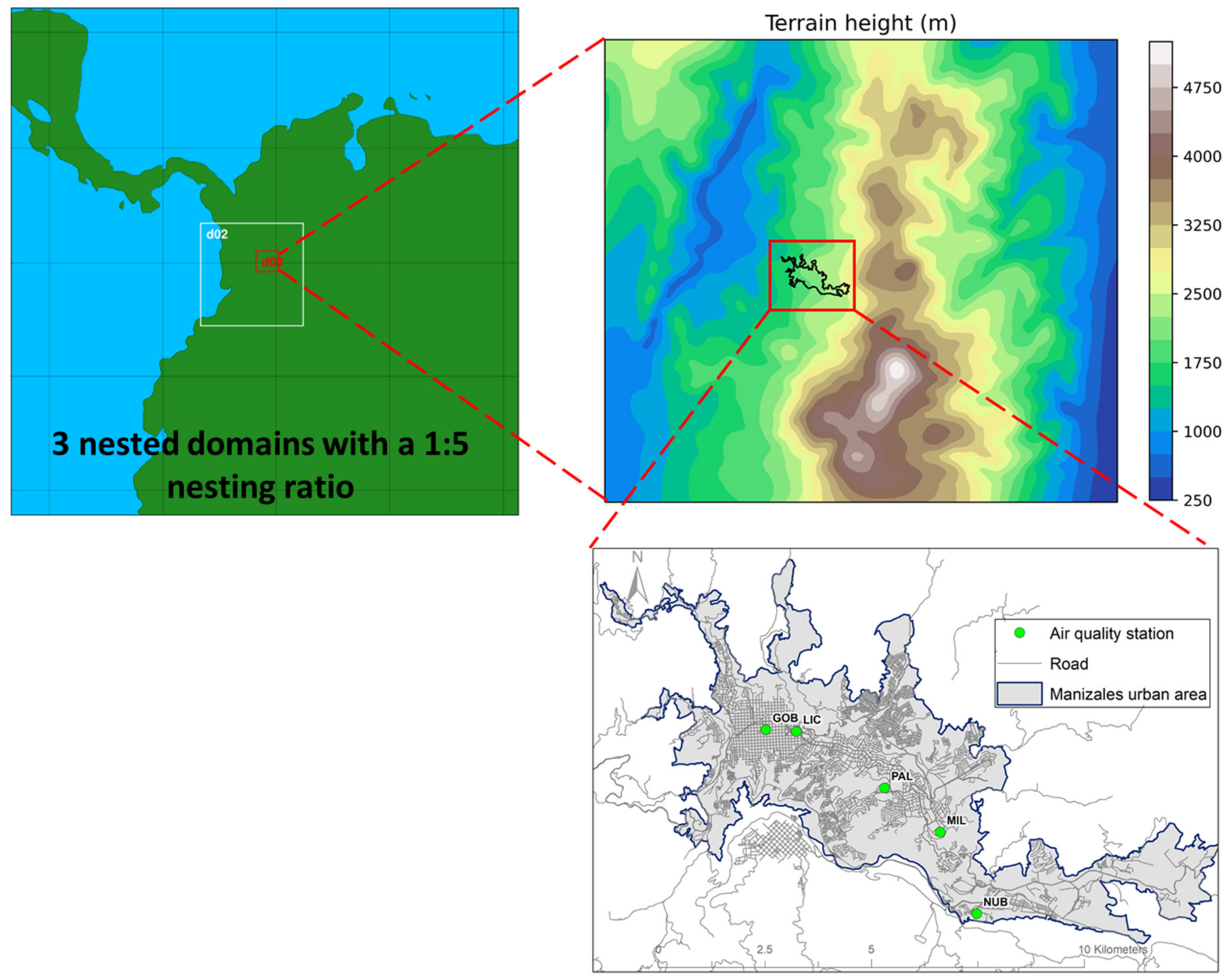
2.1. Study Area and EI Approaches

On-road mobile emission fluxes were estimated in Manizales, Colombia, and compared using different approaches and emission models. For all the estimations, the EI domain covered the Manizales urban area, and focused on the estimation of total annual fluxes (ton/year) of criteria pollutants (CO, NO_X, SO_X, PM₁₀, PM_2.5), non-methane volatile organic compounds (NMVOC) and greenhouse gases (CO₂, CH₄, N₂O). The IVE and COPERT emission models were implemented for the EI estimates; these differ mainly in that in IVE the emission factors are a function of the power bins of the vehicle engine, while in COPERT the emission factors are a function average vehicle speed. As well as other parameters such as available vehicle technologies, estimated pollutants, correction methods, and/or adjustments to local conditions show differences between the two models.

Emissions were estimated for 2017 as the base year considering a fleet of 169,142 vehicles distributed in five vehicle categories as follows: 48.3% passenger cars (PC), 47.1% motorcycles (2w) (18.5% 2 stroke and 81.5% 4 stroke), 1.5% buses, 1.4% taxis, and 1.7% trucks (65.5% small <14 ton and 34.5% large >14 ton). The disaggregated distribution by vehicle category, fuel type, and vehicle technology is shown in Table S1 of the Supplementary Materials.

Three EI estimations were compared in this study. First, a top-down EI performed with the International Vehicle Emissions (IVE) model [33,34], which is the most recent official EI reported in the city. A complete description and details of the methodology can be found in the studies by [3] and [28]. Second, a top-down EI was estimated with the COPERT model v5.4 [32,35]; in this case, the total pollutant emission flows were estimated with the model. The input information corresponds to the total number of vehicles in the vehicle fleet distributed by vehicle categories mentioned above (see Table S1). In addition, we use information of the vehicle activity data—kilometers traveled per year—(PC = 8250 km/year, 2w = 7590 km/year, buses = 55,440 km/year, taxis = 65,670 and trucks = 16,500 km/year) and average speeds in the range of 22 to 47 km/h reported by the city’s Mobility Master Plan. Regarding the characteristics of the fuel, the sulfur content of 173.89 ppm for gasoline and 26.34 ppm for diesel stands out. A complete description and details of the application of COPERT in Manizales from a top-down approach can be found in the study by [30]. It should be noted that the input activity data for the COPERT emission model were obtained from the equivalent information used in the official EI performed in Manizales with the IVE model [28]. Third, we used a bottom-up EI approach by coupling a traffic model with COPERT methodology applied in this study. In this case, the COPERT model was only used to obtain the emission factors adjusted to local conditions; all the input parameters remained the same as the previous case (COPERT top-down) except for the average vehicle speed. A sensitivity study in a range of different vehicle speeds (5 to 55 km/h) was performed with the COPERT model to obtain emission factor equations that represent the variation of emission rates as a function of velocity. The equations obtained can be accessed on the Mendeley data repository with doi:10.17632/y9n6nyzpx5.1 (accessed on 12 October 2021). The development of the bottom-up emissions model is detailed below.

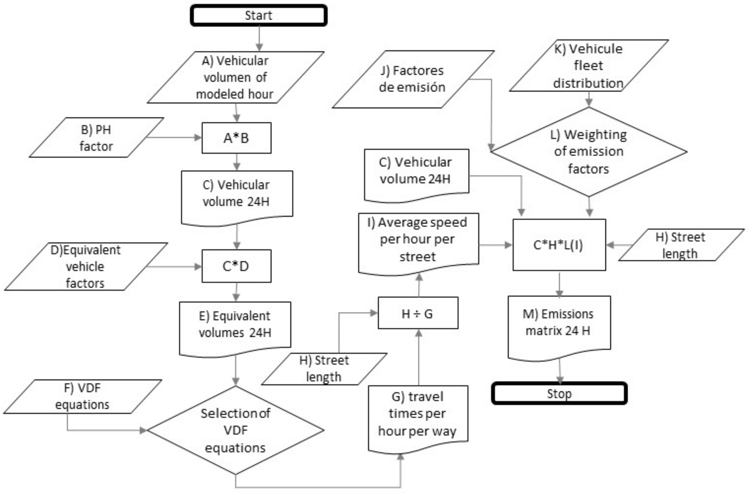
2.2. Bottom-Up Emission Model Description

The emissions inventory based on a bottom-up approach was developed by coupling a traffic model with emission factors, following a similar approach to the one proposed by [5]. Equation (1) represents the estimation of emissions:

$$E_{ij}=A{F}_T\times E{F}_{ij}\left(V\right)$$

(1)

where:

$E_{ij}$ = Emissions of pollutant (i) generated by vehicle type (j).

$A{F}_j$ = Activity factor of vehicle type (j) (kilometers traveled by the vehicle).

$E{F}_{ij}\left(V\right)$ = Emission factor of pollutant (i) by vehicle type (j) as a function of speed (V).

The emission modeling process consisted of three major steps: (i) Traffic modeling, (ii) emission factor, and (iii) emission processing. Figure 1 presents the modeling framework and process flow of the bottom-up approach.

The traffic modeling provided disaggregated activity data about traffic behavior, which is used to estimate the load of pollutants along roads in the city. In this study, we used a static traffic assignment model built in PTV-VISUM and calibrated for the morning rush hour for 2017.

Table 1. Transport modeling parameters and specifications for Manizales, Colombia.

Parameter	Description
Area of study	Manizales and 4 neighbor municipalities
Number of traffic analysis zones	409
Number of modeled nodes	2322
Number or modeled road links	6562
Modeling base year	2017
Modeled time period	6:45—7:45
Number of vehicle classes *	8, including private vehicles, taxis, motorcycles, heavy goods vehicles, light goods vehicles, urban buses, cableway, intercity buses.

* For EI estimates using the COPERT model, the relationship used is explained in Table S2 of the Supplementary Materials.

shows the main specifications of the traffic model. Inputs for the static traffic assignment model include the road network with traffic capacity and volume-delay functions, and origin–destination matrices for motorcycles, private vehicles, taxis, and trucks. Traffic flow from buses was preloaded to the network based on transit operational time-tables. We performed a multiclass traffic assignment with a stochastic route choice model. Calibration of the model was based on traffic counts (i.e., observed link-traffic flows vs. modeled link-traffic flows) using 35 link volumes for light-duty and heavy-duty vehicles. Final modeled flows were optimized in the traffic model to reflect the observed conditions of travel time and speeds in the network.

Activity factors that better represent the vehicle activity in Manizales required post-processing of traffic modeling outputs to accurately account for time variation of traffic conditions during a typical day. We computed an hourly-ratio factor between the traffic volume observed during the morning rush hour and each hour of the day (PHF), using traffic counts provided by the traffic authority in the city. We used a factor of 330 to compute annual traffic from the 24-h traffic estimates, based on the handbook for transport and traffic studies in Colombia.

Vehicle composition of the city, distinguished by vehicle type, technology, and fuel type, was obtained based on data from the official EI of the city [28]. EF by vehicle type, technology, and fuel expressed in grams of pollutant per kilometer traveled as a function of average speed were obtained using COPERT 5.4 and coupled with the traffic volumes and speeds to finally estimate the emissions. The vehicle fleet distribution in Manizales used for estimation of emissions using the COPERT model is presented in Table S1.

2.3. Air Quality Modeling

The Weather Research and Forecasting with Chemistry (WRF-Chem) model version 3.7.1 [36] was used to perform air quality simulations with the three different EIs as input information. Figure 2 shows the domain configuration of the model considering 3-nested domains (1:5 nesting ratio) with a downscaling process from 25-km resolution (parent domain) to 1-km resolution in the domain of interest, which covers the urban area of Manizales and surrounding areas. Details of model configuration are presented in Table S3, and major details about the reasons for the chosen configuration are described in the study by [18].

Emissions information was included in the WRF-Chem model after a procedure of spatial distribution of total emission fluxes in a uniform grid-cell of 1 km² and 1-h temporal resolution. The Disaggregation of on-ROad Vehicle Emissions algorithm (DROVE) [37] was used for distributing emissions into time and space. Then, the Another Assimilation System for WRF-Chem (AAS4WRF) [38,39] was used for building the WRF-Chem input emission files.

2.4. Field Observations and Air Quality Model Evaluation

Surface ambient concentrations of CO and O₃ were obtained from the Manizales air quality monitoring network (AQMN). The AQMN has one station for O₃ and CO monitoring (GOB station) in downtown Manizales and reports hourly concentrations. Furthermore, other surface AQ stations described in Figure 2 provided information of daily PM₁₀ and PM_2.5, monitored in the AQMN every three days.

Quantitative model performance evaluation (MPE) was applied for comparing observational data with simulation results. The following statistical performance metrics were calculated using the software R and the Openair package [40]: mean bias (MB), mean gross error (MGE), root mean squared error (RMSE), normalized MB (NMB), normalized MGE (NMGE), normalized RMSE (NRMSE), and Pearson correlation coefficient (r). Different studies conducted around the world have used these statistics for model evaluation purposes [18,19,23,41,42]. Definitions of statistics used in this study are presented in Equations (S1)–(S7) of the Supplementary Materials.

3. Results and Discussion

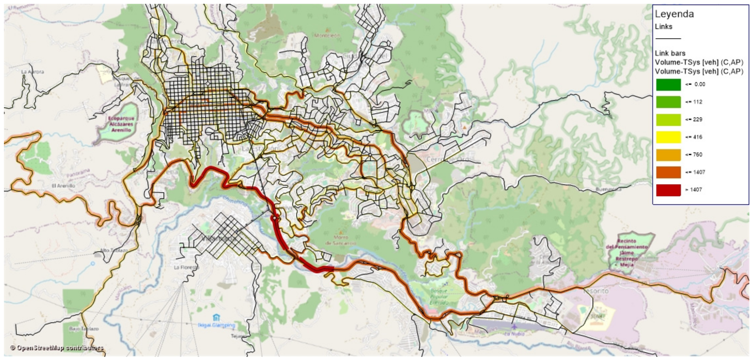
3.1. Traffic Model

Around 45,948 vehicles were assigned to the network to represent traffic conditions of the morning rush hour in Manizales (6:45—7:45 am). The traffic assignment model converged to a stable solution, thus reaching equilibrium conditions. Figure 3 shows the assigned flows and the goodness of fit in the model for private vehicles after following a state-of-the-practice transport modeling calibration process. Similar results for taxis, motorcycles, and trucks were obtained.

3.2. Total Fluxes Comparison among EI

Total annual emission fluxes estimated for Manizales (base year 2017) are shown in

Table 2. Total annual emission fluxes in the city of Manizales for the base year 2017 and contribution by vehicle category.

Vehicle Category	Pollutants
	CO	NOx	SO2	BC	PM2.5	PM10	NMVOC	VOC	CO2	N2O	CH4
IVE/Top-Down
Total emissions (ton/year)	25,082.8	4358.7	28.4	---	---	555.6	3835.8	---	517,948.0	17.8	1650.9
Passenger car	32.9%	16.2%	64.8%	---	---	3.9%	13.9%	---	40.2%	55.1%	27.7%
Motorcycle	36.6%	2.2%	18.0%	---	---	13.2%	75.9%	---	10.1%	0.0%	35.3%
Taxi	24.5%	7.4%	11.3%	---	---	1.2%	2.2%	---	15.6%	24.2%	36.9%
Bus	2.3%	38.6%	3.2%	---	---	42.4%	3.4%	---	17.2%	6.7%	0.0%
Truck	3.7%	35.6%	3.2%	---	---	39.3%	4.5%	---	16.9%	14.0%	0.1%
COPERT/Top-Down
Total emissions (ton/year)	11,483.7	2518.4	20.5	40.5	88.7	88.7	2013.5	2171.4	367,907.7	17.2	157.9
Passenger car	28.7%	18.7%	56.1%	6.4%	5.3%	5.3%	23.4%	23.2%	32.8%	75.0%	19.8%
Motorcycle	65.3%	6.5%	24.4%	11.4%	36.4%	36.4%	71.4%	70.4%	12.4%	7.0%	57.2%
Taxi	2.9%	1.5%	5.9%	0.5%	0.6%	0.6%	1.6%	1.9%	7.3%	5.2%	5.4%
Bus	2.5%	58.4%	10.7%	64.9%	45.7%	45.7%	2.6%	3.5%	37.3%	9.9%	15.0%
Truck	0.7%	14.8%	2.9%	16.5%	12.2%	12.2%	0.9%	1.1%	10.2%	2.9%	2.6%
COPERT/Bottom-Up
Total emissions (ton/year)	16,567.0	2424.8	25.2	38.6	109.6	131.9	3111.8	3132.6	414,065.4	17.3	165.7
Passenger car	33.4%	20.1%	55.9%	8.9%	12.4%	16.2%	25.3%	25.5%	36.0%	73.0%	17.1%
Motorcycle	59.6%	7.7%	26.3%	13.6%	35.1%	31.9%	67.1%	69.7%	15.1%	7.5%	58.4%
Taxi	5.2%	2.8%	7.8%	1.4%	3.2%	4.6%	5.7%	1.9%	10.2%	8.2%	10.3%
Bus	1.2%	42.7%	6.0%	47.9%	30.2%	28.8%	1.1%	1.8%	23.3%	6.7%	9.9%
Truck	0.7%	26.7%	4.0%	28.2%	19.0%	18.5%	0.9%	1.1%	15.4%	4.6%	4.3%

. Overall, the three EI agreed that CO₂, CO, and NO_X were the highest emitted pollutants. On the one hand, CO₂ and CO were mainly emitted by passenger cars, motorcycles, and taxis, thus representing more than 90% of these emissions; in addition, these vehicle categories are known for using gasoline as fuel. On the other hand, NO_X was emitted in a bigger proportion by buses and trucks, thus representing more than 70% of these emissions; in this case, these vehicles operated exclusively with diesel. The other emitted pollutants studied were ranked from the highest to the lowest in the following order: VOC, NMVOC, CH₄, PM₁₀, PM_2.5, BC, SO₂, and N₂O. Despite matching the order of the highest to the lowest emitted species, the actual values of emission fluxes, and the distribution between categories were different in each EI.

3.2.1. Effect of Estimation Approaches (Bottom-Up vs. Top-Down)

The COPERT/top-down and COPERT/bottom-up approaches exhibited considerable differences in the estimated emission fluxes. Indeed, as shown in

Table 3. Percent change of emissions between the COPERT/Bottom-up and the COPERT/Top-down EI [(Top-down—bottom-up)/bottom-up].

Vehicle Category	Percent Change
	CO	NOx	SO2	BC	PM2.5	PM10	NMVOC	VOC	CO2	N2O	CH4
Passenger car	67.8%	3.4%	22.5%	31.9%	189.8%	354.8%	66.7%	58.9%	24.0%	−2.1%	−9.5%
Motorcycle	31.6%	13.4%	32.6%	13.8%	19.3%	30.3%	45.1%	42.9%	36.8%	8.3%	7.2%
Taxi	160.8%	74.0%	63.1%	172.0%	606.2%	1106.1%	455.1%	48.8%	56.9%	57.5%	100.9%
Bus	−32.3%	−29.6%	−30.9%	−29.7%	−18.2%	−6.3%	−34.7%	−27.4%	−29.2%	−31.7%	−30.5%
Truck	56.2%	73.5%	68.5%	62.5%	92.7%	126.3%	41.0%	47.9%	70.7%	59.2%	72.4%
Total	44.3%	−3.7%	22.9%	−4.7%	23.6%	48.7%	54.5%	44.3%	12.9%	0.6%	4.9%

, the emissions of criteria pollutants were higher in the bottom-up approach than in the top-down approach for passenger cars, motorcycles, taxis, and trucks. In contrast, the emissions from buses were lower in the bottom-up approach than in the other one. According to previous studies, the differences in emissions were caused by the activity factors, which are more accurate in bottom-up approaches [43,44,45]. Overall, total emissions increased in most pollutants, except for NO_X and BC, which decreased by −3.7% and −4.7%, respectively. This reduction was caused by lower emissions from buses, which compensated for the increase in emissions of other vehicle categories. Finally, the largest differences were observed for NMVOC (54.5%), PM₁₀ (48.7%), CO (44.3%), VOC (44.3%), PM_2.5 (23.6%), and SO₂ (22.9%).

The spatial distribution of emissions was also sensitive to the different approaches. Figure 4 presents the average emission patterns for some pollutants obtained after regridding the bottom-up EI and disaggregating the top-down EI. For CO and SO₂, emissions were considerably higher (up to 152% and 103% for CO and SO_2, respectively) inside the urban area of Manizales with the bottom-up approach than with the top-down approach. Conversely, NO_X emissions were lower with the bottom-up approach than with the top-down-up approach, probably due to the reduction of NO_X emissions from buses previously discussed. Finally, PM_2.5 emissions were low with the bottom-up approach in the urban area, but increased in the west side of the city, which has a road that moves large volumes of trucks.

3.2.2. Effect of Emission Models (COPERT vs. IVE)

Total emissions of each of the studied pollutants were lower with the COPERT EI. As shown in

Table 4. Change of emissions between the IVE/top-down and the COPERT/top-down EIs [(COPERT—IVE)/IVE].

Vehicle Category	Percentual Change (COPERT—IVE/IVE)
	CO	NOx	SO2	BC	PM2.5	PM10	NMVOC	VOC	CO2	N2O	CH4
Passenger car	−60.1%	−33.2%	−37.5%	---	---	−78.5%	−11.8%	---	−42.3%	31.6%	−93.2%
Motorcycle	−18.4%	75.1%	−2.0%	---	---	−55.9%	−50.6%	---	−12.7%		−84.5%
Taxi	−94.6%	−88.0%	−62.5%	---	---	−92.5%	−62.9%	---	−66.6%	−79.1%	−98.6%
Bus	−49.4%	−12.6%	144.4%	---	---	−82.8%	−60.2%	---	53.0%	41.7%
Truck	−91.9%	−75.9%	−33.3%	---	---	−95.1%	−88.9%	---	−57.3%	−80.0%	310.0%
Total	−54.2%	−42.2%	−27.8%	---	---	−84.0%	−47.5%	---	−29.2%	−3.4%	−90.4%

, the highest differences were for CH₄ (−90.4%) and PM₁₀ (−84.0%), followed by CO (−54.2%), NMVOC (−47.5%), NO_X (−42.2%), CO₂ (−29.2%), SO₂ (−27.8%) and N₂O (−3.4%). Nonetheless, some specific vehicle categories exhibited an increase in emissions with COPERT, such as NO_X emissions in motorcycles, for instance. The differences between the inventories were associated with the base EF employed in each emission model (IVE and COPERT), and their approximation to account for activity factors—on the one hand, COPERT estimated activity based on the average traveling speed of the vehicle; on the other hand, IVE uses the Vehicle Specific Power (VSP), considering the vehicle speed, vehicle acceleration, vehicle altitude and mass, the road slope, among other variables, which could help to represent more realistically the engine stress of the vehicles.

Considering the road slope to estimate the emissions could be a key factor for obtaining an accurate estimation of emissions in a city like Manizales, characterized by steep road slopes reaching inclinations of 22%, which induces higher engine stress levels and increases the amounts of emissions. COPERT accounts for a maximum of 6% road inclinations for only two vehicular categories (buses and trucks), which is insufficient for Manizales, as suggested by [30], and could also explain the lower estimated emissions with this approach.

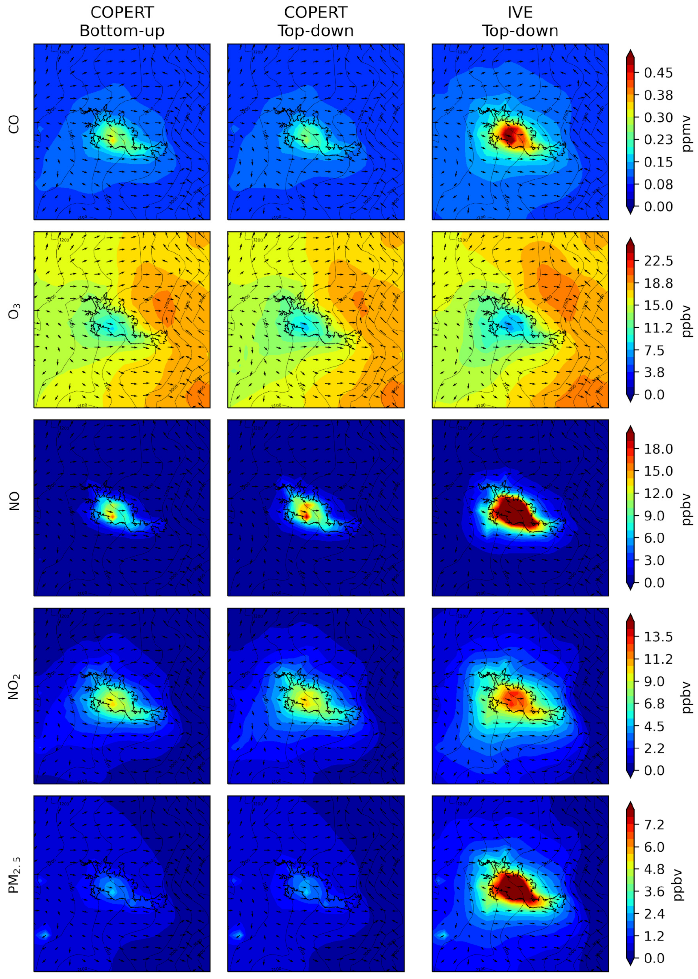
3.3. Evaluation of EI through Air Quality Modeling

3.3.1. General Results

Overall, the spatial distribution of pollutants (Figure 5) obtained with the different emission inventories was similar, with the highest concentration of CO, NO, NO₂, and PM_2.5 inside the urban area of Manizales, which is consistent with the high emissions in this area (Figure 4) caused by the activity of on-road vehicle sources. On the other hand, O₃ concentrations decreased inside the urban area of the city, which can be attributed to its high concentration of NO_X that promotes O₃ consumption.

Despite the similarities in the spatial distributions, the levels of concentrations presented significant differences, especially by comparing the IVE/top-down and the COPERT/top-down EI. For instance, CO concentrations with the IVE inventory reached a maximum value of 0.58 ppmv, while CO concentrations did not exceed the 0.28 ppm with the COPERT EI. A similar scenario was observed for NO, NO₂, and PM_2.5, all presenting higher values with the IVE EI than with the COPERT EI. The differences in the predicted concentrations were associated with the lower estimated emissions with COPERT EI than with IVE EI, as discussed in Section 3.2.2.

Analyzing the performance metrics (

Table 5. Performance metrics.

Simulation	Statistic *	Variable
		O3 [ppbv]	CO [ppmv]	PM10 [µg/m3]	PM2.5 [µg/m3]
IVE Top-down	Min	0.00	0.09	3.43	4.37
	Max	32.50	1.58	12.24	7.78
	MB	3.10	−0.23	−12.10	−6.76
	MGE	4.62	0.30	12.10	6.93
	RMSE	5.95	0.42	12.84	8.07
	NMB	0.46	−0.41	−0.62	−0.51
	NMGE	0.69	0.53	0.62	0.52
	NRMSE	1.12	1.05	2.79	1.73
	R	0.70	0.47	0.37	0.09
COPERT Top-down	Min	0.00	0.08	0.69	0.79
	Max	26.74	0.74	2.65	2.32
	MB	4.39	−0.39	−17.76	−11.89
	MGE	5.25	0.40	17.76	11.89
	RMSE	6.49	0.54	18.34	12.68
	NMB	0.65	−0.69	−0.92	−0.89
	NMGE	0.78	0.71	0.92	0.89
	NRMSE	1.22	1.35	4.08	1.65
	R	0.67	0.48	0.10	0.01
COPERT Bottom-up	Min	0.12	0.08	0.93	0.76
	Max	28.46	0.82	2.53	2.19
	MB	5.52	−0.37	−17.81	−12.01
	MGE	6.08	0.38	17.81	12.01
	RMSE	7.18	0.52	18.37	12.77
	NMB	0.82	−0.66	−0.92	−0.90
	NMGE	0.90	0.68	0.92	0.90
	NRMSE	1.35	1.30	4.09	1.66
	R	0.66	0.57	0.15	0.35

* O₃ and CO metrics correspond to model evaluation at GOB air quality station. 622 and 642 hourly records were used to validate O₃ and CO respectively. PM₁₀ and PM_2.5 metrics were obtained for daily (24 h) values. PM_2.5 metrics correspond to the values obtained at GOB air quality station, and PM₁₀ metrics were evaluated at the five air quality stations (GOB, LIC, MIL, NUB, PAL). The values presented here are averages of the performance metrics of all stations, validated through nine daily records for each station.

), the three EI represented the general trend of O₃ observations, as suggested by the moderate/strong strength correlation coefficients (R: 0.66–0.77). Indeed, the hourly profile for O₃ displayed in Figure 6 shows that the model captured the increase of concentration during the early morning (probably occasioned by transport) and around the midday (due to the higher incoming solar radiation that favors O₃ photochemical formation). Nonetheless, the model overestimated predicted values considering all the EIs (MB: 3.10 a 5.52, NMB: 0.46 a 0.82). The higher O₃ concentrations could be attributed to an underestimation of NOx emissions, which could otherwise react with O₃, thus diminishing its concentrations.

The model also captured the general trend of CO concentrations, as shown by a moderate strength correlation coefficient (R: 0.47 to 0.57). Indeed, the maximum peak concentrations during the rush traffic hours (6:00 a.m.–8:00 a.m. and 6:00 p.m.–7:00 p.m. local time) were captured with all the EIs; however, the values were underestimated (MB: −0.39 a −0.23, NMB: −0.69 a −0.41).

On the other hand, there were no measurements of NO_X in the city for the period of simulations to validate the model outputs, and values of PM_2.5 and PM₁₀ were only available as gravimetric 24-h averages from measurements taken every third day. The scarce PM₁₀ and PM_2.5 measurements showed low correlation coefficients between the modeled values and the observations (R for PM₁₀: 0.10–0.37, R for PM_2.5 0.01–0.25). Furthermore, the concentrations were underestimated (MB for PM₁₀: −12.10 to −17.81, MB for PM_2.5: −6.79 to −12.01).

3.3.2. Effect of Estimation Approach

Figure S1 presents the mean difference of concentrations for the studied pollutants between the COPERT/top-down, and the COPERT/bottom-up EIs. The results show considerable differences between both approximations. On the one hand, for CO, the bottom-up approach led to concentrations up to 25% higher than the top-down approach; on the other hand, NO, NO₂, and PM_2.5 concentrations reached maximum differences of −63%, −36%, and −13%, respectively. This behavior was caused by the difference in emission fluxes previously shown in Figure 4, where CO, NO_X, and PM_2.5 differ by 51%, −47%, and −40%, respectively, between EIs in the areas with the highest deviations. Regarding O₃ concentrations, values were higher with the bottom-up approach than with the top-down approach, probably due to the higher emissions of NO_X that enhance O₃ consumption.

Considering the representativeness of both EIs, the COPERT/bottom-up approach led to better correlation coefficients between modeled and observed values (R: 0.57 vs. 0.48) and allowed a slight reduction in the deviations of the model (MB: −0.37 vs. −0.39, NMB: −0.66 vs. −0.69). The improvements could be caused by a better distribution of activity factors throughout the day. Indeed, this is observed in the hourly profiles presented in Figure 6, as the morning peak of concentration is more prominent with the bottom-up approach.

Conversely, O₃ predictions were less precise with the bottom-up approach, as evidenced by the higher overestimation of concentrations (MB: 5.52 vs. 4.39, NMB: 0.82 vs. 0.65). The differences were higher during the nighttime, presumably due to the underestimation of NO_X emissions, which unenhanced the NO_X—O₃ titration reactions, thus leading to higher residual O₃.

3.3.3. Effect of Emission Models

Figure S2 presents the mean difference of O₃ and CO concentrations between the IVE/top-down and the COPERT/top-down EIs. CO, NO_X, and PM_2.5 concentrations (not shown in the figure) were higher with the IVE inventory, as expected due to the higher emission fluxes estimated with this approach, whose values for CO were 118% higher on average. On the other hand, O₃ concentrations were slightly lower inside the urban area of the city with the IVE EI, which could be attributed to the higher NOx concentration with IVE, thus enhancing O₃ consumption.

The differences between the IVE and COPERT EIs were associated with the base EF used by each emission model and the activity factors considered. On the one hand, COPERT used the average traveling speed of the vehicle, which is a controversial approach. Although different travels have the same average speed, they could experience different driving patterns, which modifies the levels of emission [15]. On the other hand, IVE uses the VSP approach, which considers the topography of the area (road slopes), acceleration, vehicle aerodynamics, among others [3], thus providing a better estimate of the engine stress.

Lastly, the performance metrics shown in Table 5 indicate a better model performance with the IVE EI. Indeed, the values of MB, MGE, RMSE, and R boosted for CO and O₃. Likewise, there was also an improvement in the values of MB for PM₁₀ and PM_2.5. These results suggest that the IVE approach is more representative of the conditions in Manizales.

4. Conclusions

In the present study, we estimated and compared three vehicular EIs, developed with different emission models (COPERT and IVE) and estimation approaches (Bottom-up and Top-down), and studied the differences in the estimated emission fluxes. Furthermore, all the EIs were used to perform high-resolution air quality simulations in order to validate which approximation led to the most accurate predictions of pollutants’ concentration.

The profile of emissions of on-road mobile sources was dominated by CO, CO₂, and NO_X emissions. Passenger cars, motorcycles, and taxis represent more than 90% of emissions of CO and CO₂, whereas the activity of buses and trucks mainly causes the emission of NO_X.

The different approaches led to different emission fluxes. In particular, the highest emissions were obtained with the IVE/top-down EI, followed by the COPERT/bottom-up EI for the majority of pollutants, and, lastly, the COPERT/top-down approach, which provided the lowest emission fluxes. The differences between IVE and COPERT were associated with the base EF used in each approach and the approximations considered to estimate activity factors, which are the average speed in COPERT and VSP in IVE. The discrepancies between the COPERT/top-down and the COPERT/bottom-up might be explained by the differences in activity factors throughout the day and the different city regions

The validation of the EIs through modeling suggested that CO, O₃, PM₁₀, and PM_2.5, concentrations were sensitive to the different EIs, with the most accurate performance obtained by the IVE/top-down EI. Our results suggest that the VSP approach is more representative for the conditions of Manizales, as it allows accounting for the impact of the road slopes. On the other hand, the COPERT approach lacks this ability, as it only accounts for road slopes with maximum inclinations of 6% and only for buses and trucks. Regarding the COPERT inventories, the best performance was obtained by the COPERT/bottom-up EI, as it enhanced CO, PM₁₀, and PM_2.5 performance compared with the COPERT /top-down EI. Improvements could be attributed to a better distribution of activity factors throughout the day and for the different regions of the city.

References

1. D’Angiola, A.; Dawidowski, L.E.; Gómez, D.R.; Osses, M. On-road traffic emissions in a megacity. Atmos. Environ. 2010, 44, 483–493. [Google Scholar] [CrossRef]
2. González, C.; Gómez, C.; Rojas, N.; Acevedo, H.; Aristizábal, B. Relative impact of on-road vehicular and point-source industrial emissions of air pollutants in a medium-sized Andean city. Atmos. Environ. 2017, 152, 279–289. [Google Scholar] [CrossRef]
3. González, C.M. Dinámica e Impacto de Emisiones Antrópicas y Naturales en una Ciudad Andina Empleando un Modelo Euleriano de Transporte Químico Online. Caso de Estudio: Manizales, Colombia. Ph.D. Thesis, Universidad Nacional de Colombia, sede Manizales, Manizales, Colombia, 2017. (In Spanish). [Google Scholar]
4. Pachón, J.E. Revisión de metodologías usadas para la elaboración de inventarios de emisiones atmosféricas en Colom-bia: Caso de estudio Bogotá. In Proceedings of the IV Congreso Colombiano y Conferencia Internacional de Calidad del Aire y Salud Publica, Bogotá, Colombia, 22 August 2013. (In Spanish). [Google Scholar]
5. Mangones, S.C.; Jaramillo, P.; Fischbeck, P.; Rojas, N.Y. Development of a high-resolution traffic emission model: Lessons and key insights from the case of Bogotá, Colombia. Environ. Pollut. 2019, 253, 552–559. [Google Scholar] [CrossRef] [PubMed]
6. EEA—European Environment Agency. EMEP/EEA Air Pollutant Emission Inventory Guidebook; European Environment Agency: Copenhagen, Denmark, 2016. [Google Scholar]
7. Krecl, P.; Targino, A.C.; Landi, T.P.; Ketzel, M. Determination of black carbon, PM2.5, particle number and NOx emission factors from roadside measurements and their implications for emission inventory development. Atmos. Environ. 2018, 186, 229–240. [Google Scholar] [CrossRef]
8. Pérez-Martínez, P.J.; de Miranda, R.M.; Nogueira, T.; Guardani, M.L.; Fornaro, A.; Ynoue, R.; Andrade, M.F. Emission factors of air pollutants from vehicles measured inside road tunnels in São Paulo: Case study comparison. Int. J. Environ. Sci. Technol. 2014, 11, 2155–2168. [Google Scholar] [CrossRef] [Green Version]
9. Corvaian, R.M.; Urrutia, C.M. Emission Factors for Gasoline Light-Duty Vehicles: Experimental Program in Santiago, Chile. J. Air Waste Manag. Assoc. 2000, 50, 2102–2111. [Google Scholar] [CrossRef] [PubMed]
10. Ramirez-Gamboa, J.; Pachón, J.E.; Leuro, O.M.C.; González, S.F. A new database of on-road vehicle emission factors for Colombia: A case study of Bogotá. CT F-Cienc. Tecnol. Futuro 2019, 9, 73–82. [Google Scholar] [CrossRef]
11. Londoño, J.; Correa, M.A.; Palacio, C.A. Estimación de las emisiones de contaminantes atmosféricos provenientes de fuentes móviles en el área urbana de Envigado, Colombia. Rev. Esc. Ing. Antioq. 2011, 16, 149–162. (In Spanish) [Google Scholar]
12. Peñaloza, N.E. Distribución Espacial y Temporal del Inventario de Emisiones Provenientes de las Fuentes Móviles y Fijas de la Ciudad de Bogotá, D.C. Master’s Thesis, Universidad Nacional de Colombia, Sede Bogotá, Bogotá, Colombia, 2010. (In Spanish). [Google Scholar]
13. Minambiente—Ministerio de Ambiente y Desarrollo Sostenible. Guía Para la Elaboración de Inventarios de Emisiones Atmosféricas; Dirección de Asuntos Ambientales, Sectorial y Urbana: Bogotá, Colombia, 2017. (In Spanish) [Google Scholar]
14. Pu, Y.; Yang, C.; Liu, H.; Chen, Z.; Chen, A. Impact of license plate restriction policy on emission reduction in Hangzhou using a bottom-up approach. Transp. Res. Part D: Transp. Environ. 2015, 34, 281–292. [Google Scholar] [CrossRef]
15. Wang, H.; Fu, L. Developing a High-Resolution Vehicular Emission Inventory by Integrating an Emission Model and a Traffic Model: Part 1—Modeling Fuel Consumption and Emissions Based on Speed and Vehicle-Specific Power. J. Air Waste Manag. Assoc. 2010, 60, 1463–1470. [Google Scholar] [CrossRef] [Green Version]
16. Dios, M.; Souto, J.A.; Casares, J.J.; Gallego, N.; Saez, A.; Macho, M.L.; Cartelle, D.; Vellòn, J.M. A mixed top-down and bottom-up methodology in spatial segregation of emissions based on GIS tools. Air Pollut. XX 2012, 157, 225. [Google Scholar]
17. EEA—European Environment Agency. The Application of Models under the European Union’s Air Quality Directive: A Technical Reference Guide; Technical Report No 10/2011; European Environment Agency: Copenhagen, Denmark, 2011. [Google Scholar]
18. Cifuentes, F.; González, C.; Aristizábal, B. Insights to WRF-Chem sensitivity in a zone of complex terrain in the tropical Andes: Effect of boundary conditions, chemical mechanisms, nesting, and domain configuration. Atmos. Pollut. Res. 2021, 12, 101093. [Google Scholar] [CrossRef]
19. González, C.; Ynoue, R.; Vela, A.V.; Rojas, N.; Aristizábal, B. High-resolution air quality modeling in a medium-sized city in the tropical Andes: Assessment of local and global emissions in understanding ozone and PM10 dynamics. Atmos. Pollut. Res. 2018, 9, 934–948. [Google Scholar] [CrossRef]
20. Zarate, E.; Carlos, B.L.; Clappier, A.; Manzi, V.; Bergh, H.V.D. Air quality modelling over Bogota, Colombia: Combined techniques to estimate and evaluate emission inventories. Atmos. Environ. 2007, 41, 6302–6318. [Google Scholar] [CrossRef] [Green Version]
21. Dias, D.; Amorim, J.H.; Sá, E.; Borrego, C.; Fontes, T.; Fernandes, P.; Pereira, S.R.; Bandeira, J.; Coelho, M.; Tchepel, O. Assessing the importance of transportation activity data for urban emission inventories. Transp. Res. Part D Transp. Environ. 2018, 62, 27–35. [Google Scholar] [CrossRef]
22. Li, X.; Lopes, D.; Mok, K.M.; Miranda, A.; Yuen, K.-V.; Hoi, K.I. Development of a road traffic emission inventory with high spatial–temporal resolution in the world’s most densely populated region—Macau. Environ. Monit. Assess. 2019, 191, 239. [Google Scholar] [CrossRef]
23. Kumar, A.; Jimenez, R.; Belalcazar, L.; Rojas, N. Application of WRF-Chem Model to Simulate PM10 Concentration over Bogota. Aerosol Air Qual. Res. 2016, 16, 1206–1221. [Google Scholar] [CrossRef] [Green Version]
24. Zhang, S.; Wu, Y.; Huang, R.; Wang, J.; Yan, H.; Zheng, Y.; Hao, J. High-resolution simulation of link-level vehicle emissions and concentrations for air pollutants in a traffic-populated eastern Asian city. Atmos. Chem. Phys. 2016, 16, 9965–9981. [Google Scholar] [CrossRef] [Green Version]
25. DANE—Departamento Administrativo Nacional de Estadística. Censo Nacional de Población y Vivienda 2018. Población Ajustada Por Cobertura. 2019. Available online: https://www.dane.gov.co/index.php/estadisticas-por-tema/demografia-y-poblacion/censo-nacional-de-poblacion-y-vivenda-2018/informacion-tecnica (accessed on 25 November 2019).
26. Carn, S.A.; Fioletov, V.E.; McLinden, C.; Li, C.; Krotkov, N. A decade of global volcanic SO2 emissions measured from space. Sci. Rep. 2017, 7, srep44095. [Google Scholar] [CrossRef] [PubMed] [Green Version]
27. Cuesta-Mosquera, A.P.; Wahl, M.; Acosta-López, J.G.; García-Reynoso, J.A.; Aristizábal-Zuluaga, B.H. Mixing layer height and slope wind oscillation: Factors that control ambient air SO2 in a tropical mountain city. Sustain. Cities Soc. 2020, 52, 101852. [Google Scholar] [CrossRef]
28. Corpocaldas—Corporación Autónoma Regional de Caldas; Unal—Universidad Nacional de Colombia. Aplicación de Herramientas de Simulación Atmosférica en el Estudio de la Calidad del Aire en Manizales; Informe—Convenio 107-2018; Corporación Autónoma Regional de Caldas; Universidad Nacional de Colombia, sede Manizales: Manizales Caldas, Colombia, 2020. (In Spanish) [Google Scholar]
29. Corpocaldas—Corporación Autónoma Regional de Caldas; Unal—Universidad Nacional de Colombia. Apoyo y Fortalecimiento de la Red de Monitoreo de Calidad del Aire en la Ciudad de Manizales y Cuantificación de Emisiones Atmosféricas Por Fuentes Móviles; Informe—Convenio 130-2014; Corporación Autónoma Regional de Caldas; Universidad Nacional de Colombia, sede Manizales: Manizales Caldas, Colombia, 2016. (In Spanish) [Google Scholar]
30. Trejos, E.M. Estimación de Emisiones Atmosféricas Por Fuentes Móviles en Ruta Aplicando la Metodología COPERT y Determinación de las Emisiones de Material Particulado Susceptible de Resuspensión con Información Local (Manizales—Año Base 2017). Master’s Thesis, Universidad Nacional de Colombia, sede Manizales, Manizales, Colombia, 2021. (In Spanish). [Google Scholar]
31. Mangones, S.C.; Jaramillo, P.; Rojas, N.Y.; Fischbeck, P. Air pollution emission effects of changes in transport supply: The case of Bogotá, Colombia. Environ. Sci. Pollut. Res. 2020, 27, 35971–35978. [Google Scholar] [CrossRef]
32. Emisia SA—Conscious of Transport’s Impact. EMISIA SA/Utilities/COPERT/COPERT Download. 2021. Available online: https://www.emisia.com/utilities/copert/versions/; https://www.emisia.com/utilities/copert/download/ (accessed on 14 May 2021).
33. Davis, N.; Lents, J.; Osses, M.; Nikkila, N.; Barth, M. Development and application of an international vehicle emissions model. In Proceedings of the Transportation Research Board 81st Annual Meeting, Washington, DC, USA, 13–17 January 2002; Available online: http://www.issrc.org/ive/downloads/presentations/IVE_TRB_2005.pdf (accessed on 14 May 2021).
34. ISSRC (International Sustainable Research Center). IVE Model Users Manual. Version 2.0. 2008. Available online: http://www.issrc.org/ive/downloads/manuals/UsersManual.pdf (accessed on 26 February 2021).
35. EEA—European Environment Agency. EMEP/EEA Air Pollutant Emission Inventory Guidebook 2019—Update October 2020. 1.A.3.b.i-iv Road Transport. 2019. Available online: https://www.eea.europa.eu/publications/emep-eea-guidebook-2019/part-b-sectoral-guidance-chapters/1-energy/1-a-combustion/1-a-3-b-i/view (accessed on 26 February 2021).
36. Grell, G.A.; Peckham, S.E.; Schmitz, R.; McKeen, S.A.; Frost, G.; Skamarock, W.C.; Eder, B. Fully coupled “online” chemistry within the WRF model. Atmos. Environ. 2005, 39, 6957–6975. [Google Scholar] [CrossRef]
37. González, C.M.; Gómez, C.D.; Aristizábal, B.H. DROVE: An Algorithm for Spatial and Temporal Disaggregation of On-road Vehicle Emission Inventories. Aerosol Air Qual. Res. 2020, 20, 2765–2779. [Google Scholar] [CrossRef]
38. Vara-Vela, A.; Muñoz, A.; Lomas, A.S.; González, C.M.; Calderon, M.G.; Andrade, M.D.F. The Another Assimilation System for WRF-Chem (AAS4WRF): A New Mass-Conserving Emissions Preprocessor for WRF-Chem Regional Modelling. In Proceedings of the AGU Fall Meet, New Orleans, LA, USA, 11–15 December 2017. [Google Scholar]
39. Vara-Vela, A.; Andrade, M.F.; Kumar, P.; Ynoue, R.Y.; Muñoz, A.G. Impact of vehicular emissions on the formation of fine particles in the Sao Paulo Metropolitan Area: A numerical study with the WRF-Chem model. Atmos. Chem. Phys. Discuss. 2016, 16, 777–797. [Google Scholar] [CrossRef] [Green Version]
40. Carslaw, D.C.; Ropkins, K. Openair—An R package for air quality data analysis. Environ. Model. Softw. 2012, 27–28, 52–61. [Google Scholar] [CrossRef]
41. Borge, R.; Alexandrov, V.; del Vas, J.J.; Lumbreras, J.; Rodríguez, E. A comprehensive sensitivity analysis of the WRF model for air quality applications over the Iberian Peninsula. Atmos. Environ. 2008, 42, 8560–8574. [Google Scholar] [CrossRef]
42. Hoshyaripour, G.; Brasseur, G.; Andrade, M.; Gavidia-Calderón, M.; Bouarar, I.; Ynoue, R. Prediction of ground-level ozone concentration in São Paulo, Brazil: Deterministic versus statistic models. Atmos. Environ. 2016, 145, 365–375. [Google Scholar] [CrossRef]
43. Aparicio, L.G.C.; Pérez, M.A.R.; Robles, A.M.C.; Remolina, B.R.G.; Pulido, H.E.S.; Forero, R.A.M.; Quinche, J.E.P. Conciliación de inventarios top-down y bottom-up de emisiones de fuentes móviles en Bogotá, Colombia. Rev. Tecnura 2016, 20, 59–74. [Google Scholar] [CrossRef] [Green Version]
44. Ibarra-Espinosa, S.; Ynoue, R.; O’Sullivan, S.; Pebesma, E.; Andrade, M.D.F.; Osses, M. VEIN v0.2.2: An R package for bottom–up vehicular emissions inventories. Geosci. Model Dev. 2018, 11, 2209–2229. [Google Scholar] [CrossRef]
45. Wang, H.; Fu, L.; Lin, X.; Zhou, Y.; Chen, J. A bottom-up methodology to estimate vehicle emissions for the Beijing urban area. Sci. Total Environ. 2009, 407, 1947–1953. [Google Scholar] [CrossRef] [PubMed]
Figure 1. Bottom-up emission estimation modeling approach.
Atmosphere 12 01372 g001
Figure 2. Emission inventory domain (bottom-right) and configuration of model simulation with three domains (up-left). The zoom map is shown for the fine-grid domain D3 (top-right). The urban area of Manizales city (bottom-right) includes the location of monitoring stations used for model evaluation.
Atmosphere 12 01372 g002
Figure 3. Volume assignment for private vehicles.
Atmosphere 12 01372 g003
Figure 4. Spatial distribution of emissions of the COPERT/bottom-up and COPERT/top-down EIs, and difference map (bottom-up minus top-down).
Atmosphere 12 01372 g004
Figure 5. Average concentration of CO, O3, NO, NO2, and PM2.5 for the period of simulation.
Atmosphere 12 01372 g005
Figure 6. Average hourly profiles of CO, O3, NO, NO2, and PM2.5 at GOB station.
Atmosphere 12 01372 g006