Disturbances of the Thermosphere and the Ionosphere during a Meteorological Storm

Abstract

Determination of the physical mechanisms of energy transfer of tropospheric disturbances to the ionosphere is one of the fundamental problems of atmospheric physics. This article presents the results of observations carried out using two-wavelength lidar sensing at tropospheric altitudes and satellite GPS measurements during a meteorological storm in Kaliningrad (Russia, 54.7° N, 20.5° E) on 1 April 2016. During lidar sensing, it was found that the amplitudes of variations in atmospheric parameters with periods of acoustic (AWs) and internal gravity (IGWs) waves significantly increased. As a result of numerical modeling using the AtmoSym software package, it was shown that there is a noticeable increase in the period of temperature disturbances from 6–12 min to 10–17 min at altitudes from 150 km up to 230 km during the vertical propagation of acoustic waves and internal gravity waves from the troposphere. Nonlinear and dissipative processes in this layer lead to the formation of sources of secondary waves in the thermosphere with periods longer than those of primary ones. In this case, the unsteady nature of the wave source and the short duration of its operation does not lead to significant heating of the thermosphere. Simultaneous satellite observations demonstrate the response of the ionosphere (total electron content (TEC) disturbance) to tropospheric disturbances. Analysis of the time series of the amplitudes of the reflected lidar signal and TEC made it possible to determine that the response time of the ionosphere to tropospheric disturbances is 30–40 min.

1. Introduction

One of the fundamental problems of physics of the atmosphere is the determination of correlations between the dynamic processes occurring in the lower atmosphere and changes in the plasma parameters of the ionosphere and establishing physical mechanisms of energy transfer from the troposphere to the thermosphere and ionosphere. Various tropospheric processes excite waves in the neutral atmosphere. Upward propagating waves in the lower atmosphere and their modifications, interactions and modulations affect the ionosphere when and if they reach it. Those waves are planetary, tidal, gravity, and acoustic waves [1,2,3,4,5].

Existing hypotheses about the processes that determine the influence of processes in the lower atmosphere on the state of the thermosphere and ionosphere are based on the concept of the generation of AWs and IGWs in the troposphere and spreading them vertically upwards [6,7,8,9,10]. The sources of such waves in the lower atmosphere may be different. For example, it may be the mesoscale turbulence, convection [5,11], disturbances arising in the atmosphere due to stationary incoming air streams flowing around mountains (orography effects) [12,13], earthquakes and seismic activity [7,14,15], the passage of the solar terminator and solar eclipse [16,17,18,19,20], meteorological disturbances and typhoon [1,21,22,23,24,25,26,27,28,29].

The reaction of the thermosphere and ionosphere parameters to these events reveals, particularly, in the formation of ionospheric irregularities over the region of disturbances in the lower atmosphere, the appearance of traveling ionospheric disturbances, disturbances in electric fields, optical emissions, F-expansion phenomena, etc. [24,30,31,32,33,34,35,36,37]. These phenomena in the thermosphere and ionosphere develop relatively quickly, i.e., within a few hours after the occurrence of disturbances near the Earth’s surface [1,5,6,38,39]. The processes of generation, propagation, and influence of AWs and IGWs on the atmosphere have been studied theoretically in numerous works [40,41,42]. The theoretical concepts can be confirmed by simultaneous experimental studies of dynamic processes in the lower and upper atmosphere with the spatial and temporal resolution, making it possible to distinguish disturbances with the specific characteristics of AWs and IGWs.

Lidar sensing methods are widely used in atmospheric dynamics studies. By their principle of operation, they can be divided into four classes, i.e., aerosol lidars (Rayleigh lidars), Raman scattering lidars (Raman lidars), resonance effect lidars (including metal fluorescence lidars), and lidars based on differential absorption of scattered radiation. The Rayleigh lidar operation scheme [43,44,45] is based on the combination of a receiver and a radiation source, which makes it possible to change the zenith angle and sensing azimuth. Several variants of systems are used for sensing, i.e., single-wave, multi-wave, and polarization ones. The variety of presented systems is associated with the importance of obtaining information on the physical parameters of atmospheric aerosols, which often determine the type of pollution. Raman lidar is used to measure a range of atmospheric molecules, including N₂, O₂, H₂O, SO₂, and CO₂ [46]. Its use requires powerful lasers, large telescopes, long accumulation times and is usually limited to measurements of high molecular concentrations.

Lidar based on resonance effects is characterized by careful selection of both the laser radiation wavelength and the radiation wavelength recorded by the receiver so that they coincide with the wavelength of the absorption line of the investigated atmospheric component. Excitation of a molecule at the absorption frequency leads to resonant scattering, which can be much more intense than non-resonant scattering. This method has been successfully used to measure atomic sodium and potassium concentrations at high altitudes [47,48]. The operation of lidar on the differential absorption of scattered radiation depends on scattering by atmospheric aerosols, but measurements of the selected type of molecules are carried out by their absorption [49]. The method uses at least two laser beams with different wavelengths, which are successively or simultaneously sent along the same direction into the atmosphere. The first laser beam is absorbed by the molecules under investigation, while the second beam with a similar wavelength is not very strongly absorbed. Since the beams differ in a small wavelength interval, the aerosol scattering cross-sections can be considered practically the same for both cases. The difference in the intensity of scattering of rays in the atmosphere can be considered due to their absorption by the studied molecules. Analysis of the recorded signals from both beams as a function of time allows for spatially resolved measurements of the concentration of absorbing molecules. The advantages of lidar sensing are the high spatial and temporal resolution of measurements, as far as the possibility of long-term observations.

In experimental studies of the ionosphere, methods for analyzing the total electron content (TEC), determined from observations of signals from satellites of the GPS/GLONASS global navigation satellite systems, are effectively used [50,51,52,53,54,55,56,57]. Such observations provide a high temporal resolution of measurements performed by individual stations.

Numerical modeling is an important tool for the theoretical study of wave processes in the atmosphere. At present, the development of computer technology and the improvement of methods for the numerical integration of hydrodynamic equations make it possible to build models for the generation and propagation of AWs and IGWs in the atmosphere, taking into account nonlinear and dissipative processes, as well as real stratification of the medium, for example [5,9,58,59]. In theoretical research [59,60,61,62,63], it was established that the heat release/absorption processes occurring due to phase transitions of water in the atmosphere during the formation and evolution of clouds and the development of other meteorological phenomena have a significant effect on the state of the thermosphere and ionosphere. However, a significant problem in numerical studies of wave processes in the atmosphere is determining realistic sources of disturbances, as far as the initial and boundary conditions. One possible solution to this problem would be using observational data of atmospheric parameters during the focused period. For example, in [64,65], the correctness of the mathematical model of AWs propagation from the lower atmosphere upward using the observed pressure variations on the surface as boundary conditions was justified. A correct description has also approved the accuracy of the numerical model of atmospheric disturbances during the passage of the atmospheric front over the Moscow region.

This work aims to study the influence of a meteorological storm on the dynamics of the thermosphere and ionosphere. The article presents an analysis of the results of observations made with the use of lidar sensing at tropospheric heights, TEC variations, reconstructed from satellite GPS measurements, and also presents the results of numerical modeling on thermospheric disturbances caused by observed variations in atmospheric pressure in the troposphere during a meteorological storm in Kaliningrad on 1 April 2016.

2. Lidar and Satellite Measurements

The question about the geomagnetic conditions is very important when conducting this kind of experiment. Quiet geomagnetic conditions are a prerequisite to perform a refined experiment since TEC disturbances resulting from AW and IGW propagation from the troposphere can be hidden by the TEC variations caused by geomagnetic storms. Moreover, even weak geomagnetic activity can cause strong and long-term disturbances in the thermosphere [66], potentially affecting the TEC value. However, from the data presented below, it follows that the characteristic times of the observed rapid changes in the thermosphere and ionosphere are much shorter than the time of development of post-storm effects, which last for several days during the recovery phase.

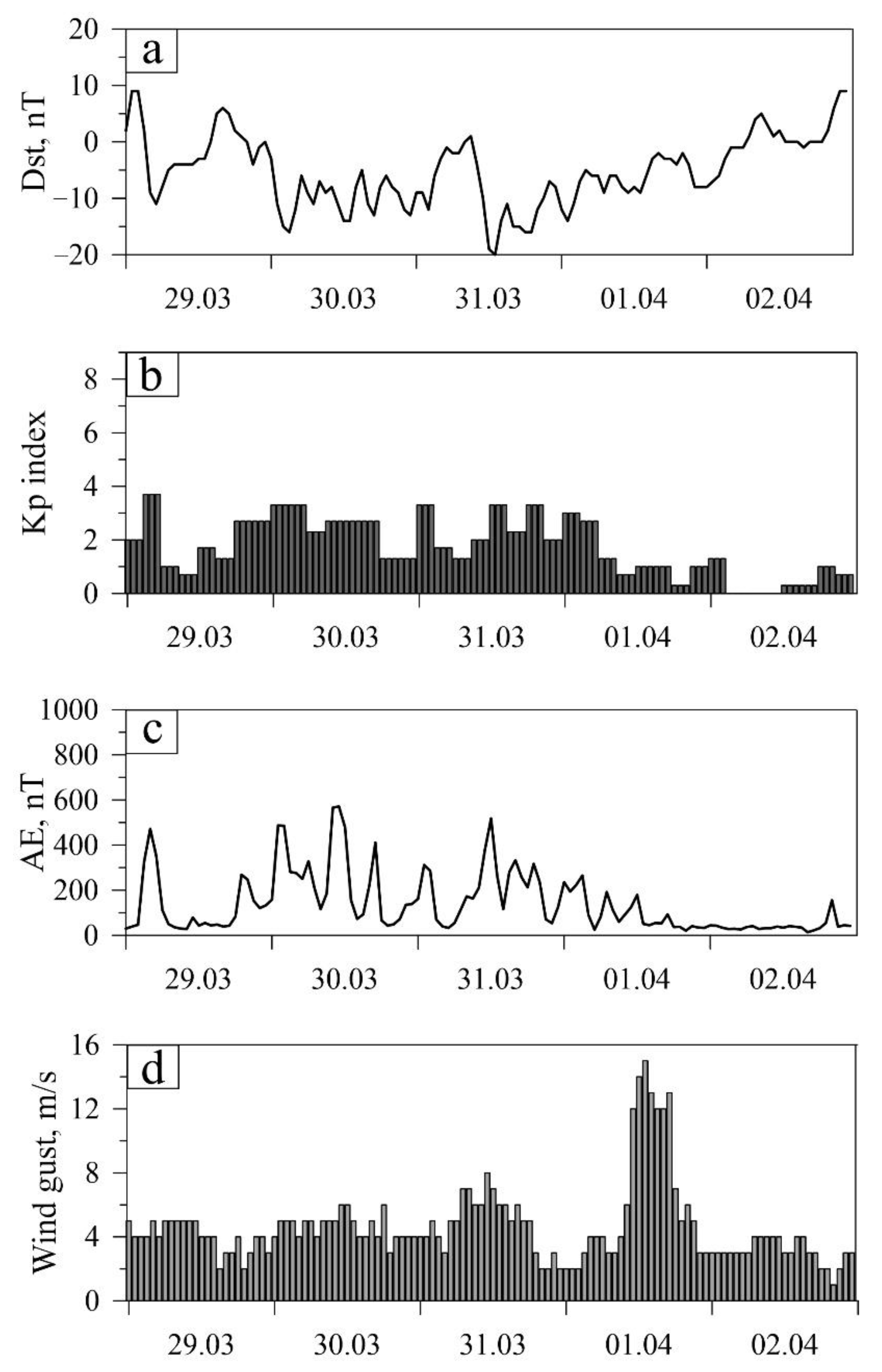
2.1. Geomagnetic Conditions during the Experiment

The geomagnetic conditions from 29 March to 2 April 2016 are presented in Figure 1 following the SPDF-OMNIWeb service (https://omniweb.gsfc.nasa.gov, accessed on 15 September 2021). It can be seen that they were quiet on the eve and during the meteorological storm in Kaliningrad on 1 April 2016. Thus, the Dst index varied from −20 to 10 nT (no more than 20 nT per day), the Kp index did not exceed 3.3, and the AE index did not exceed 500 nT. At the same time, on March 31, there was an increase in wind gusts up to 8 m/s, and on 1 April 2016, from 12:00 to 19:00 UTC, wind gusts reached 14 m/s, which corresponds to a meteorological storm. On calm days, 29 and 30 March, and 2 April 2016, a weak and moderate wind with a speed of 2–4 m/s was observed.

2.2. Lidar Measurement Technique

Lidar sensing of tropospheric aerosols was carried out at the KLGD station (Kaliningrad, Russia, 54.7° N, 20.5° E). For observations, we used a two-wave Rayleigh lidar LSA-2S (Obninskaya Photonika Ltd., Obninsk, Russia), which makes it possible to determine the characteristics of aerosols at distances up to 20 km. Lidar LSA-2S has the following technical characteristics: emitter is Nd: YAG-laser LS-2131 with two operating wavelengths of 1064 nm and 532 nm, with pump energy of up to 25 J and a pulse repetition rate of no more than 20 Hz. The Cassegrain-type receiver with the main mirror of the receiving telescope 260 mm in diameter and a focal length of 1050 mm was used for backscattered radiation. The measurement time for one aerosol profile was no more than 1 min. The photodetector for the 1064 nm channel had a photocathode efficiency of 40% and an interfilter half-width of 3 nm. The FEU-10 photomultiplier with a photocathode quantum efficiency of 10% and a transmission half-width of 2 nm was used for the second channel at 532 nm.

A software package [67], which implements an algorithm using parametric correlation dependences between the integral characteristics over the spectrum of aerosol sizes, and the ratio of the backscattering coefficients at the sensing wavelengths [68], has been applied to analyze the LSA-2S measurement results.

Spectral analysis of the time series obtained in the observations makes it possible to determine the frequency ranges of variations in atmospheric parameters at different altitudes. The function F(t), which is the difference in signal intensities for different strobes, was used to study the dynamics of the selected atmospheric layers:

$$F(t)=f_{m+1}(t)-f_m(t).$$

(1)

where $f_m(t)$ is the intensity of the scattered signal in the strobe with the number m, t is the observation time.

For F(t), the wavelet transform of the function is applied using the Morlet wavelet transform as the kernel. Direct integral wavelet transform of a signal is the scalar transformation of the signal and is the result of multiplication of the signal and the kernel of the transformation, which is a function ψ of the given type. Function W(a,b) is the wavelet image of the signal F(t) on independent variables a and b:

$$W(a,b)={\displaystyle \underset{-\infty }{\overset{\infty }{\int }}F(t){\psi }_{ab}}(t)dt,$$

(2)

$${\psi }_{ab}(t)={\left|a\right|}^{-1/2}\psi \left(\frac{t-a}{b}\right);a,b\in R;\psi (t)\in L^2(R).$$

(3)

The analytical representation of the Morlet wavelet is:

$$\psi (t)=\exp \left(i{k}_{0}t\right)\exp \left(-\frac{t^2}{2}\right).$$

(4)

Parameters b and a determine the period and time-shift of disturbances in the analyzed series F(t). The most frequently used basis is derived on the Morlet wavelet localized in k- and t- space. The change in W(a,b) with time makes it possible to see the types of wave disturbances and the time of their appearance [69].

2.3. Technique of Satellite GPS Measurements

TEC is one of the key parameters of the ionosphere state. To assess the disturbances in the ionosphere, we used the data of GPS observations at the mid-latitude station LAMA (Lamkovko, Poland, 53.9° N, 20.7° E). In the present work, we utilized the method for determining the TEC from code measurements of the pseudorange at $f_1=1575.42$ MHz and $f_2=1227.60$ MHz GPS carrier frequencies, described in detail in [70,71].

The characteristic periods of the arising ionospheric disturbances were calculated using the Morlet wavelet analysis (1)–(4) of the current TEC variations, determined from observations with a step of 30 s. A more detailed description of the algorithm for studying the frequency characteristics of TEC variations is given in [25].

2.4. Determination of the Parameters of a Meteorological Storm

The parameters of the meteorological storm were determined using the ERA5 reanalysis [72], which provides hourly estimates of a large amount of data on the atmosphere, Earth’s surface and ocean. Reanalysis is a method of generating comprehensive information about how weather and climate change over time. Currently, reanalysis is actively used by numerical weather prediction centers. It objectively combines observations and a numerical model, generates a synthesized assessment of the system state, and produces a new, improved forecast.

Figure 2 shows a map of wind gusts according to ERA5 data on 1 April 2016, at 15:00 UTC. As can be seen from Figure 2, the characteristic spatial size of the meteorological disturbance reached 500 km.

2.5. Results of Experiments

Figure 3 shows the results of wavelet analysis of variations in the intensity of the lidar signal scattered in the atmosphere at an altitude of ~5650 m in observations made on 1 April 2016, during the period of wind intensification in the troposphere over Kaliningrad and variations in TEC above the LAMA station, obtained from signals attained by PRN 13 and PRN 24 satellites.

This choice of GPS satellites is due to the proximity of the projections of their trajectory to the observation station (see Figure 2). The flight of satellites was recorded in the daytime (about noon), making it possible to exclude the effects of the solar terminator on the Earth’s ionosphere.

Analysis of the data in Figure 3 suggests that the response of the ionosphere to an increase in the amplitudes of tropospheric disturbances with a period of 3–5 min at 11:35–12:40, 13:00–13:40, and after 14:00 UTC are TEC disturbances with periods 10–17 min at 12:05–12:40, 13:00–13:45 and after 14:40 UTC, respectively. Note that the characteristic response time of the ionosphere to tropospheric disturbances is 30–40 min.

Experimental observations of wave variations in the ionosphere during intensifying cyclonic activity reveal variations with AWs and IGWs periods in TEC observations. It can be assumed that rapid changes in the meteorological situation under storm conditions create favorable conditions for AW and IGW excitation in a wide range of periods. Propagation of AWs and IGWs into the thermosphere and their dissipation cause the observed disturbances of the ionosphere.

3. Numerical Simulation

A numerical experiment to study the influence of meteorological disturbances in Kaliningrad on 1 April 2016, on the thermosphere was carried out using a regional two-dimensional version of the high-resolution model AtmoSym [58,73,74]. The version used in these calculations is based on the solution of a system of two-dimensional nonlinear hydrodynamic equations for atmospheric gas, where the horizontal position of the point is specified by the x coordinate and the vertical one by the z coordinate. A detailed description of AtmoSym is given in [75]. This model is non-hydrostatic and has a high resolution in time (~0.1 s) and space (vertical grid spacing~500 m), which allows studying a wide range of atmospheric waves, including AWs and IGWs [76,77,78]. AtmoSym considers the real stratification of the atmosphere, nonlinear and dissipative processes of different scales, describes the formation of shock waves and turbulent processes. Currently, AtmoSym is actively used to research atmospheric wave disturbances [8,78,79,80,81].

An unsolved problem remains an adequate description of meteorological sources of waves in the atmosphere in terms of modeling vertical wave propagation. However, the most developed approach to describing these kinds of sources is presented in [75]. In this work, a mathematical formulation of the problem of waves propagation in the atmosphere initiated by pressure fluctuations associated with meteorological processes on the lower boundary of the region of integration of equations has been formulated, and its correctness has been proved. The results of numerical calculations on modeling atmospheric disturbances during the passage of a meteorological front using the observed data of surface pressure variations showed reasonable agreement with the observational data [64,65].

In practice, it is not always possible to obtain data on pressure variations by direct measurements; therefore, the use of experimental data on the intensity of the lidar signal, as was done in work [63], reduced to the data on pressure variations in the surface layer is effective. Variations in lidar signal intensity reflect the frequency response of pressure variations at a fixed altitude. The amplitude values of pressure variations were calculated according to the assumption that the maximum amplitudes of changes in the observed intensity of the scattered signal corresponding to the amplitudes of pressure variations in the spring. The following function approximates the source:

$$f_p(t,x)=\exp \left[-{\left(\frac{x-x_0}{d}\right)}^2\right]f(t),$$

(5)

where f(t) is time-dependent approximated experimental data, d is the source width, and f_p(t,x) is the pressure variations near the Earth’s surface. Function f(t) is the pressure variations obtained from the lidar signal intensity observational data described in the previous section. They are assumed to reflect the frequency response of pressure variations at a fixed height. The maximum amplitude intensity changes in the scattered signal correspond to the amplitudes of pressure variations from 780 Pa on 1 April 2016, in Kaliningrad. The applied procedure contains inaccuracy in determining the amplitude values of pressure variations, so the amplitude variations of pressure during the passage of meteorological fronts described, for example, in [65,82], differ from those obtained in the calculations for the investigated storm. We assume that the inaccuracy in determining the amplitude does not affect the frequency characteristics of disturbances in the surface atmosphere. The calculated pressure on the Earth’s surface is shown in Figure 4. As can be seen, the increase in the amplitudes of pressure variations at 11:30–12:40, 13:00–13:40, and after 14:00 UTC reflects the wavelet analysis results of disturbances at tropospheric heights (see Figure 3).

Thus, the conditions on the Earth’s surface (the lower boundary of the region of integration of the model) have the form:

$$u(x,z=0,t)=0,$$

(6)

$$\frac{\partial w(x,z=0,t)}{\partial z}=0,$$

(7)

$$T(x,z=0,t)=T_0(0),$$

(8)

$$P(x,z=0,t)=P_0(0)+f_p(x,t),$$

(9)

where u, w are horizontal and vertical velocity components, respectively, T-–T₀ is the background temperature, P is pressure, P₀ is the background pressure, f_p(x,t) is the approximated function of pressure change at the Earth’s surface. The computational domain has a vertical scale of 500 km and a horizontal scale of 3000 km. A local source with a width of d = 300 km is located in the region’s center.

4. Analysis of Wave Variations in the Atmosphere and Discussion

The features of the appearance of waves generated by tropospheric sources are similar for various events. Infrasonic wave components excited by tropospheric sources are the first to reach the heights of the thermosphere. As can be seen from Figure 3, the appearance of AWs and IGWs in the thermosphere and ionosphere occurs 30–40 min after the beginning of their amplification in the troposphere. In this case, due to nonlinear and dissipative processes in the thermosphere, thermospheric disturbances are formed with characteristic spatial and temporal scales exceeding the size of the region of tropospheric disturbances. Numerical calculations in a neutral atmosphere for the investigated meteorological event demonstrate the development of the wave pattern described above.

Analysis of temperature disturbances at heights of the thermosphere and in the region of the tropospheric source shows (see Figure 5) that at the initial stage of calculations short-period disturbances in the thermosphere repeat the tropospheric disturbances with a delay, which is typical for acoustic waves. Over time, differences appear like temperature changes in the thermosphere and troposphere, which are associated with the tropospheric source’s nonstationarity and nonlinear and dissipative processes in the thermosphere.

The spatial structure of temperature perturbations in the atmosphere 1 h after switching on the source of perturbations is shown in Figure 6. As can be seen from the figure, immediately above the disturbance region, cooling regions below 300 km and heating regions above 400 km are formed. The spatial proportions of these regions are somewhat larger than the size of the disturbance source in the lower atmosphere.

These areas are formed due to the vertical propagation of waves from the lower atmosphere. We also note the appearance of wave disturbances with characteristic wavelengths of ~200 km, propagating almost horizontally from the disturbance region in the thermosphere. The appearance of these disturbances is due to the dissipation processes of waves coming from the lower atmosphere and the excitation of secondary atmospheric waves directly in the thermosphere [5], as well as waveguide propagation of waves with appropriate periods. As shown in work [77], waves with periods less than the Brent-Väisälä period can be captured into the waveguide at heights where this period is longer than that for the incoming waves. Figure 5 and Figure 6 show that the unsteady nature of the wave source and the short duration of its operation doesn’t lead to significant heating of the thermosphere. Nevertheless, it can be noted that positive temperature perturbations in Figure 6 exceed the amplitudes of negative perturbations, which is explained by the contribution of dissipative processes.

Figure 7 shows temperature perturbations at an altitude of 300 km above the source of perturbations in the lower atmosphere and a point displaced by 500 km. As can be seen from the figure, the disturbances above the source region in the thermosphere repeat their non-stationary character (see Figure 3a,b), while at the shifted point, the process is characterized by quasi-harmonic damped oscillations with a period of ~20 min.

Figure 8 shows temperature perturbations at an altitude of 250 km at various times during the operation of the perturbation source. As can be seen from the figure, the region of thermospheric disturbances is ±500 km from the disturbance epicenter. At large distances from the source, the perturbations are quasi-harmonic, damped oscillations with a characteristic wavelength of ~200 km.

Figure 9 presents the temperature variations over the epicenter of the disturbance source. Disturbances in the thermosphere generally reflect the development of the excitation of atmospheric waves in the lower atmosphere (see Figure 4). In this case, a time delay in the appearance of disturbances at high altitudes can be noted, which is due to the vertical propagation of waves, as well as an increase in the period of disturbances with height with an increase in the duration of the source.

Figure 10 shows the results of wavelet analysis of temperature perturbations at an altitude of 150 and 230 km above the source of perturbations. As shown in Figure 9, waves with periods of 6–12 min prevail at an altitude of 150 km and 10–16 min at 230 km. An increase in wave activity is observed half an hour after the start of the source operation. Such results obtained for a neutral atmosphere in numerical calculations practically correspond to the data of TEC observations considered in Section 2 (see Figure 3).

The numerical experiment results showed that AWs and IGWs excited by surface pressure disturbances during periods of meteorological disturbances propagate into the thermosphere and lead to changes in its state. In theoretical studies, the effects of AWs and IGWs propagation into the thermosphere have been studied sufficiently. The results of experimental and model studies obtained in this work confirm these assumptions.

In experimental studies of the spectra of disturbances in the ionosphere associated with meteorological events, it was shown that in these periods, there is an increase in the amplitudes of TEC variations with periods of 2–20 and 20–60 min [33,83] Analysis of the results of observations and numerical experiments suggests that the disturbances in the thermosphere generated by tropospheric sources have two frequency ranges. The first high-frequency range is determined by the short-period IGWs and AWs, which form the disturbance parameters directly above the tropospheric source. With large time scales, the second low-frequency range is determined by the duration of the action of waves coming from the lower atmosphere and the excitation of secondary IGWs directly in the thermosphere in the processes of dissipation of tropospheric wave dissipation [78,84,85,86].

5. Conclusions

This paper presents the results of observations carried out using lidar sensing at tropospheric heights and satellite GPS measurements during the meteorological storm in Kaliningrad (Russia) on 1 April 2016. The results of lidar sensing allow us to assert that during the period of a meteorological storm, the amplitudes of variations in atmospheric parameters with AW and IGW periods increase significantly. Simultaneous satellite observations demonstrate the response of the ionosphere (TEC disturbance) to tropospheric disturbances. Analysis of the time series of the amplitudes of the reflected lidar signal and TEC made it possible to determine that the response time of the ionosphere to tropospheric disturbances is 30–40 min.

As a result of numerical modeling, it was found that during the vertical propagation of AWs and IGWs upward from the troposphere, there is a noticeable increase in the period of temperature disturbances from 6–12 min to 10–17 min at altitudes from 150 km to 230 km. In this layer, nonlinear and dissipative processes lead to the formation of secondary wave sources in the thermosphere, with periods longer than those of primary ones. In this case, the unsteady nature of the primary wave source and the short duration of its operation doesn’t lead to significant heating of the thermosphere, i.e., the energy of the primary waves is spent mainly on the excitation of secondary waves.

The reaction of the ionosphere (variations in the integral TEC parameter) to tropospheric disturbances occurs somewhat later than variations in the parameters of the thermosphere (in particular, temperature) at an altitude of 230 km. However, the periods of temperature variations above 230 km and TEC variations differ little since there is a close relationship between the thermosphere and ionosphere parameters [87].

References

1. Laštovička, J. Forcing of the ionosphere by waves from below. J. Atmos. Sol. Terr. Phys. 2006, 68, 479–497. [Google Scholar] [CrossRef]
2. Forbes, J.M.; Maute, A.; Zhang, X.; Hagan, M.E. Oscillation of the ionosphere at planetary-wave periods. J. Geophys. Res. Space Phys. 2018, 123, 7634–7649. [Google Scholar] [CrossRef]
3. Rishbeth, H.; Mendillo, M. Patterns of F2-Layer Variability. J. Atmos. Sol. Terr. Phys. 2001, 63, 1661–1680. [Google Scholar] [CrossRef]
4. Yiǧit, E.; Koucká Knížová, P.; Georgieva, K.; Wardm, W. A review of vertical coupling in the Atmosphere-Ionosphere system: Effects of waves, sudden stratospheric warmings, space weather, and of solar activity. J. Atmos. Sol. Terr. Phys. 2016, 141, 1–12. [Google Scholar] [CrossRef]
5. Fritts, D.C.; Alexander, M.J. Gravity wave dynamics and effects in the middle atmosphere. Rev. Geophys. 2003, 41. 1003:1–1003:64. [Google Scholar] [CrossRef] [Green Version]
6. Pertsev, N.N.; Shalimov, S.L. Generation of atmosphere gravitation waves in the seismically active region and their effect on the ionosphere. Geomagn. Aeron. 1996, 36, 111–118. [Google Scholar]
7. Klimenko, M.; Klimenko, V.V.; Karpov, I.V.; Zakharenkova, I.E. Simulation of seismo-ionospheric effects initiated by internal gravity wave. Russ. J. Phys. Chem. B 2011, 5, 393–401. [Google Scholar] [CrossRef]
8. Karpov, I.V.; Kshevetskii, S.P. Formation of large-scale disturbances in the upper atmosphere caused by acoustic gravity wave sources on the Earth’s surface. Geomagn. Aeron. 2014, 54, 513–522. [Google Scholar] [CrossRef]
9. Hickey, M.P.; Schubert, G.; Walterscheid, R.L. Acoustic wave heating of the thermosphere. J. Geophys. Res. Space Phys. 2001, 106, 21543–21548. [Google Scholar] [CrossRef] [Green Version]
10. Drobzheva, Y.; Krasnov, V. Acoustic energy transfer to the upper atmosphere from surface chemical and underground nuclear explosions. J. Atmos. Sol. Terr. Phys. 2006, 68, 578–585. [Google Scholar] [CrossRef]
11. Fritts, D.; Vadas, S.L.; Wan, K.; Werne, J.A. Mean and variable forcing of the middle atmosphere by gravity waves. J. Atmos. Sol. Terr. Phys. 2006, 68, 247–265. [Google Scholar] [CrossRef]
12. Gavrilov, N.; Koval, A. Parameterization of mesoscale stationary orographic wave forcing for use in numerical models of atmospheric dynamics. Izv. Atmos. Ocean. Phys. 2013, 49, 244–251. [Google Scholar] [CrossRef]
13. Gavrilov, N.; Koval, A.; Pogoreltsev, A.I.; Savenkova, E.N. Numerical modeling of inhomogeneous orographic wave influence on planetary waves in the middle atmosphere. Adv. Space Res. 2013, 51, 2145–2154. [Google Scholar] [CrossRef]
14. Astafyeva, E. Ionospheric detection of natural hazards air plasma parameters in normal and seismic conditions. Rev. Geophys. 2019, 57, 1265–1288. [Google Scholar] [CrossRef]
15. Shalimov, S.; Rozhnoi, A.; Solov’eva, M.; Olshanskaya, E. Impact of earthquakes and tsunamis on the ionosphere. Izv. Phys. Sol. Earth 2019, 55, 168–181. [Google Scholar] [CrossRef]
16. Jakowski, N.; Stankov, S.; Wilken, V.; Borries, C.; Altadill, D.; Chum, J.; Buresova, D.; Boska, J.; Sauli, P.; Hruska, F.; et al. Ionospheric behavior over Europe during the solar eclipse of October 3, 2005. J. Atmos. Sol. Terr. Phys. 2008, 70, 836–853. [Google Scholar] [CrossRef]
17. Altadill, D.; Sole, J.G.; Apostolov, E.M. Vertical structure of a gravity wave like oscillation in the ionosphere generated by the solar eclipse. J. Geophys. Res. 2001, 10, 21419–21428. [Google Scholar] [CrossRef]
18. Jones, T.B.; Wright, D.M.; Milner, J.; Yeoman, T.K.; Reid, T.; Chapman, P.J.; Senior, A. The detection of atmospheric waves produced by the total solar eclipse of August 11, 1999. J. Atmos. Sol. Terr. Phys. 2004, 66, 363–374. [Google Scholar] [CrossRef] [Green Version]
19. Kumar, K.V.; Ajeet, K.M.; Kumar, S.; Singh, R. July 22, 2009, Total Solar Eclipse induced gravity waves in the ionosphere as inferred from GPS observations over EIA. Adv. Space Res. 2016, 58, 1755–1762. [Google Scholar] [CrossRef]
20. Rybnov, Y.; Soloviev, S. Synchronous variations in the atmospheric pressure and electric field during the passage of the solar terminator. Geomagn. Aeron. 2019, 59, 234–241. [Google Scholar] [CrossRef]
21. Zakharov, V.I.; Kunitsyn, V.E. Regional features of atmospheric manifestations of tropical cyclones according to ground-based GPS network data. Geomagn. Aeron. 2012, 52, 533–545. [Google Scholar] [CrossRef]
22. Kazimirovsky, E.S. Coupling from below as a source of ionospheric variability: A review. Ann. Geophys. 2002, 45, 1–29. [Google Scholar] [CrossRef]
23. Koucká Knížová, P.; Mošna, Z.; Kouba, D.; Potužníková, K.; Boška, J. Influence of meteorological systems on the ionosphere over Europe. J. Atmos. Sol. Terr. Phys. 2015, 136, 244–250. [Google Scholar] [CrossRef]
24. Chernigovskaya, M.A.; Shpynev, B.G.; Ratovsky, K.G. Meteorological effects of ionospheric disturbances from vertical radio sounding data. J. Atmos. Sol. Terr. Phys. 2015, 136, 235–243. [Google Scholar] [CrossRef]
25. Borchevkina, O.; Karpov, I.; Karpov, M. Meteorological storm influence on the ionosphere parameters. Atmosphere 2020, 11, 1017. [Google Scholar] [CrossRef]
26. Plougonven, R.; Zhang, F. Internal gravity waves from atmospheric jets and fronts. Rev. Geophys. 2014, 52, 33–76. [Google Scholar] [CrossRef] [Green Version]
27. Karpov, I.V.; Borchevkina, O.P.; Karpov, M.I. Local and regional ionospheric disturbances during meteorological disturbances. Geomagn. Aeron. 2019, 59, 458–466. [Google Scholar] [CrossRef]
28. Karpov, I.V.; Karpov, M.I.; Borchevkina, O.P.; Yakimova, G.A.; Korenkova, N.A. Spatial and temporal variations of the ionosphere during meteorological disturbances in December 2010. Russ. J. Phys. Chem. B 2019, 13, 714–719. [Google Scholar] [CrossRef]
29. Koucká Knížová, P.; Podolská, K.; Potužníková, K.; Boška, J.; Kozubek, M. Evidence of vertical coupling: Meteorological storm Fabienne on 23 September 2018 and its related effects observed up to the ionosphere. Ann. Geophys. 2020, 38, 73–93. [Google Scholar] [CrossRef] [Green Version]
30. Martinis, C.R.; Manzano, J.R. The influence of active meteorological systems on the ionosphere F region. Ann. Geofis. 1999, 42, 1–7. [Google Scholar] [CrossRef]
31. Isaev, N.; Kostin, V.; Belyaev, G.; Ovcharenko, O.; Trushkina, E. Disturbances of the topside ionosphere caused by typhoons. Geomagn. Aeron. 2010, 50, 243–255. [Google Scholar] [CrossRef]
32. Isaev, N.; Sorokin, V.; Chmyrev, V.; Serebryakova, O.N.; Yashchenko, A.K. Disturbance of the electric field in the ionosphere by sea storms and typhoons. Cosmic Res. 2002, 40, 547–553. [Google Scholar] [CrossRef]
33. Polyakova, A.S.; Perevalova, N.P. Comparative analysis of TEC disturbances over tropical cyclone zones in the North-West Pacific Ocean. Adv. Space Res. 2013, 52, 1416–1426. [Google Scholar] [CrossRef]
34. Chou, M.Y.; Lin, C.C.H.; Yue, J.; Tsai, H.F.; Sun, Y.Y.; Liu, J.Y.; Chen, C.H. Concentric traveling ionosphere disturbances triggered by Super Typhoon Meranti (2016). Geophys. Res. Lett. 2017, 44, 1219–1226. [Google Scholar] [CrossRef]
35. Li, W.; Yue, J.; Yang, Y.; Li, Z.; Guo, J.; Pan, Y.; Zhang, K. Analysis of ionospheric disturbances associated with powerful cyclones in East Asia and North America. J. Atmos. Sol. Terr. Phys. 2017, 161, 43–54. [Google Scholar] [CrossRef]
36. Hocke, K.; Schlegel, K. A review of atmospheric gravity waves and travelling ionospheric disturbances: 1982–1995. Ann. Geophys. 1996, 14, 917–940. [Google Scholar] [CrossRef]
37. Golubkov, G.V.; Bychkov, V.L.; Gotovtsev, V.O.; Adamson, S.O.; Dyakov, Y.A.; Rodionov, I.D.; Golubkov, M.G. Glow of Heavy Dust Particles in Earth’s Atmosphere during an Earthquake. Russ. J. Phys. Chem. B 2020, 14, 351–354. [Google Scholar] [CrossRef]
38. Karpov, M.I.; Karpov, I.V.; Borchevkina, O.P.; Yakimova, G.A.; Korenkova, N.A. Ionospheric disturbances during meteorological storms. Geomagn. Aeron. 2020, 60, 611–618. [Google Scholar] [CrossRef]
39. Borchevkina, O.P.; Korenkova, N.A.; Leshchenko, V.S.; Klimenko, M.K.; Karpov, I.V.; Radievskii, A.V.; Bessarab, F.S.; Vlasov, V.I.; Kotova, D.S.; Nosikov, I.A.; et al. Complex of radiophysical, geomagnetic, and meteorological observations (IZMIRAN), Kaliningrad Branch. Russ. J. Phys. Chem. B 2020, 14, 883–891. [Google Scholar] [CrossRef]
40. Grigoriev, G.I. Acoustic-gravity waves in the Earth’s atmosphere (Review). Radiophys. Quant. Electron. 1999, 42, 1–21. [Google Scholar] [CrossRef]
41. Nekrasov, A.; Shalimov, S.; Shukla, P.K.; Stenflo, L. Nonlinear disturbances in the ionosphere due to acoustic gravity waves. J. Atmos. Terr. Phys. 1995, 57, 737–741. [Google Scholar] [CrossRef]
42. Yigit, E.; Medvedev, A.S. Internal wave coupling processes in Earth’s atmosphere. Adv. Space Res. 2015, 55, 983–1003. [Google Scholar] [CrossRef] [Green Version]
43. Khaykin, S.M.; Hauchecorne, A.; Mze, N.; Keckhut, P. Seasonal variation of gravity wave activity at midlatitudes from 7 years of COSMIC GPS and Rayleigh lidar temperature observations. Geophys. Res. Lett. 2015, 42, 1251–1258. [Google Scholar] [CrossRef]
44. Mze, N.; Hauchecorne, A.; Keckhut, P.; Thetis, M. Vertical distribution of gravity wave potential energy from long-term Rayleigh lidar data at a northern middle-latitude site. J. Geophys. Res. Atmos. 2014, 119, 12069–12083. [Google Scholar] [CrossRef]
45. Gong, S.; Yang, G.; Xu, J.; Liu, X.; Li, Q. Gravity wave propagation from the stratosphere into the mesosphere studied with lidar, meteor radar, and TIMED/SABER. Atmosphere 2019, 10, 81. [Google Scholar] [CrossRef] [Green Version]
46. Matvienko, G.G.; Babushkin, P.A.; Bobrovnikov, S.M.; Borovoi, A.G.; Bochkovskii, D.A.; Galileiskii, V.P.; Grishin, A.I.; Dolgii, S.I.; Elizarov, A.I.; Kokarev, D.V.; et al. Laser and optical sounding of the atmosphere. Atmos. Ocean. Opt. 2020, 33, 51–68. [Google Scholar] [CrossRef]
47. Yuan, T.; Heale, C.J.; Snively, B.; Cai, X.; Pautet, P.D.; Fish, C.; Zhao, Y.; Tailor, M.J.; Pendleton, W.R., Jr.; Wickwar, V.; et al. Evidence of dispersion and refraction of a spectrally broad gravity wave packet in the mesopause region observed by the Na lidar and mesospheric temperature mapper above Logan, Utah. J. Geophys. Res. Atmos. 2015, 121, 579–594. [Google Scholar] [CrossRef] [Green Version]
48. Huang, K.M.; Liu, H.; Liu, A.Z.; Zhang, S.D.; Huang, C.M.; Gong, Y.; Ning, W.H. Investigation on spectral characteristics of gravity waves in the MLT using lidar observations at Andes. J. Geophys. Res. Space Phys. 2021, 126. e2020JA028918:1–e2020JA028918:18. [Google Scholar] [CrossRef]
49. Weitkamp, C. Lidar: Range-Resolved Optical Remote Sensing of the Atmosphere; Springer: New York, NY, USA, 2005; p. 456. ISBN 978-0-387-40075-4. [Google Scholar] [CrossRef]
50. Azeem, I.; Vadas, S.L.; Crowley, G.; Makela, J.J. Traveling ionospheric disturbances over the United States induced by gravity waves from the 2011 Tohoku tsunami and comparison with gravity wave dissipative theory. J. Geophys. Res. Space Phys. 2017, 122, 3430–3447. [Google Scholar] [CrossRef]
51. Shalimov, S.L.; Olshanskaya, E.V. On Ionospheric Variations Recorded by GPS during Meteotsunami. Izv. Atmos. Ocean. Phys. 2020, 56, 576–584. [Google Scholar] [CrossRef]
52. Chen, J.; Zhang, X.; Ren, X.; Zhang, J.; Freeshah, M.; Zhao, Z. Ionospheric disturbances detected during a typhoon based on GNSS phase observations: A case study for typhoon Mangkhut over Hong Kong. Adv. Space Res. 2020, 66, 1743–1753. [Google Scholar] [CrossRef]
53. Yasyukevich, Y.V.; Kiselev, A.V.; Zhivetiev, I.V.; Edemskiy, I.K.; Syrovatskii, S.V.; Maletckii, B.M.; Vesnin, A.M. SIMuRG: System for Ionosphere Monitoring and Research from GNSS. GPS Solut. 2020, 24, 69. [Google Scholar] [CrossRef]
54. Golubkov, G.V.; Manzhelii, M.I.; Lushnikov, A.A. Radiochemical physics of the upper Earth’s atmosphere. Russ. J. Phys. Chem. B 2014, 8, 604–611. [Google Scholar] [CrossRef]
55. Golubkov, G.V.; Manzhelii, M.I.; Berlin, A.A.; Lushnikov, A.A. Fundamentals of radiochemical physics of the Earth’s atmosphere. Russ. J. Phys. Chem. B 2016, 10, 77–90. [Google Scholar] [CrossRef]
56. Kuverova, V.V.; Adamson, S.O.; Berlin, A.A.; Bychkov, V.L.; Dmitriev, A.V.; Dyakov, Y.A.; Eppelbaum, L.V.; Golubkov, G.V.; Lushnikov, A.A.; Manzhelii, M.I.; et al. Chemical physics of D and E layers of the ionosphere. Adv. Space Res. 2019, 64, 1876–1886. [Google Scholar] [CrossRef]
57. Golubkov, G.V.; Manzhelii, M.I.; Berlin, A.A.; Bezuglov, N.N.; Klyucharev, A.N.; Borchevkina, O.P.; Adamson, S.O.; Dyakov, Y.A.; Karpov, I.V.; Morozov, I.I.; et al. Remote sensing of the Earth’s surface using GPS signals. Russ. J. Phys. Chem. B 2021, 15, 362–365. [Google Scholar] [CrossRef]
58. Kshevetskii, S.P. Analytical and numerical investigation of nonlinear internal gravity waves. Nonlin. Proc. Geophys. 2001, 8, 37–53. [Google Scholar] [CrossRef] [Green Version]
59. Akhmedov, R.R.; Kunitsyn, V.E. Simulation of the ionospheric disturbances caused by earthquakes and explosions. Geomagn. Aeron. 2004, 44, 95–101. [Google Scholar]
60. Yigit, E.; Medvedev, A.S.; Aylward, A.D.; Hartogh, P.; Harris, M.J. Modeling the effects of gravity wave momentum deposition on the general circulation above the turbopause. J. Geophys. Res. Atmos. 2009, 114. D07101:1–D07101:14. [Google Scholar] [CrossRef]
61. Gavrilov, N.M.; Kshevetskii, S.P.; Koval, A.V. Verifications of the high-resolution numerical model and polarization relations of atmospheric acoustic-gravity waves. Geosci. Mod. Dev. 2015, 8, 1831–1838. [Google Scholar] [CrossRef] [Green Version]
62. Dyakov, Y.A.; Kurdyaeva, Y.A.; Borchevkina, O.P.; Karpov, I.V.; Adamson, S.O.; Golubkov, G.V.; Olkhov, O.A.; Peskov, V.D.; Rodionov, A.I.; Rodionova, I.P.; et al. Vertical propagation of acoustic gravity waves from the lower atmosphere during a solar eclipse. Russ. J. Phys. Chem. B 2020, 14, 355–361. [Google Scholar] [CrossRef]
63. Kurdyaeva, Y.; Borchevkina, O.; Karpov, I.; Kshevetskii, S. Thermospheric disturbances caused by the propagation of acoustic-gravity waves from the lower atmosphere during a solar eclipse. Adv. Space Res. 2021, 68, 1390–1400. [Google Scholar] [CrossRef]
64. Kurdyaeva, Y.; Kulichkov, S.; Kshevetskii, S.; Borchevkina, O.; Golikova, E. Propagation to the upper atmosphere of acoustic-gravity waves from atmospheric fronts in the Moscow region. Ann. Geophys. 2019, 37, 447–454. [Google Scholar] [CrossRef] [Green Version]
65. Kshevetskii, S.; Kurdyaeva, Y.; Kulichkov, S.; Borchevkina, O.; Gavrilov, N. Simulation of propagation of acoustic-gravity waves generated by tropospheric front instabilities into the upper atmosphere. Pure Appl. Geophys. 2020, 177, 5567–5584. [Google Scholar] [CrossRef]
66. Cai, X.; Burns, A.G.; Wang, W.; Qian, L.; Solomon, S.C.; Easters, R.W.; Pedatella, N.; Daniell, R.E.; McClintock, W.E. The two-dimensional evolution of thermospheric ΣO/N2 response to weak geomagnetic activity during solar-minimum observed by GOLD. Geophys. Res. Lett. 2020, 47. e2020GL088838:1–e2020GL088838:9. [Google Scholar] [CrossRef]
67. Korshunov, V.A. Automated algorithm of data processing of two-wavelength lidar sensing at slant paths. Ecol. Syst. Dev. 2009, 12, 3–10. [Google Scholar]
68. Korshunov, V.A. Retrieval of integral parameters of tropospheric aerosol from two-wavelength lidar sensing. Izv. Atmos. Ocean. Phys. 2007, 43, 618–633. [Google Scholar] [CrossRef]
69. Astafyeva, N.M. Wavelet analysis: Basic theory and some applications. Phys. Usp. 1996, 39, 1085–1108. [Google Scholar] [CrossRef]
70. Shagimuratov, I.I.; Chernyak, Y.V.; Zakharenkova, I.E.; Yakimova, G.A. Use of total electron content maps for analysis of spatial-temporal structures of the ionosphere. Russ. J. Phys. Chem. B 2013, 7, 656–662. [Google Scholar] [CrossRef]
71. Shagimuratov, I.I.; Cherniak, Y.V.; Zakharenkova, I.E.; Yakimova, G.A.; Tepenitsyna, N.Y.; Efishov, I.I. Internet service for generating GPS/GLONASS maps of ionospheric total electron content over the European region. Sovr. Probl. Dist. Zond. Zeml. Kosm. 2016, 13, 197–209. [Google Scholar] [CrossRef]
72. Hersbach, H.; Bell, B.; Berrisford, P.; Hirahara, S.; Horányi, A.; Muñoz-Sabater, J.; Nicolas, J.; Peubey, C.; Radu, R.; Schepers, D.; et al. The ERA5 global reanalysis. Q. J. R. Met. Soc. 2020, 146, 1999–2049. [Google Scholar] [CrossRef]
73. Kshevetskii, S.P. Modeling of propagation of internal gravity waves in gases. Comput. Math. Math. Phys. 2001, 41, 273–288. [Google Scholar]
74. Kshevetskii, S.P. Numerical simulation of nonlinear internal gravity waves. Comput. Math. Math. Phys. 2001, 12, 1777–1791. [Google Scholar]
75. Kurdyaeva, Y.A.; Kshevetskii, S.P.; Gavrilov, N.M.; Kulichkov, S.N. Correct Boundary Conditions for the High-Resolution Model of Nonlinear Acoustic-Gravity Waves Forced by Atmospheric Pressure Variations. Pure Appl. Geophys. 2018, 175, 3639–3652. [Google Scholar] [CrossRef]
76. Gavrilov, N.M.; Kshevetskii, S.P. Three-dimensional numerical simulation of nonlinear acoustic-gravity wave propagation from the troposphere to the thermosphere. Earth Planets Space 2014, 66. 88:1–88:8. [Google Scholar] [CrossRef] [Green Version]
77. Karpov, I.; Kshevetskii, S. Numerical study of heating the upper atmosphere by acoustic-gravity waves from a local source on the Earth’s surface and influence of this heating on the wave propagation conditions. J. Atmos. Sol. Terr. Phys. 2017, 164, 89–96. [Google Scholar] [CrossRef]
78. Kshevetskii, S.P.; Kulichkov, S.N. Effects of internal gravity waves from convective clouds on atmospheric pressure and spatial temperature-disturbance distribution. Izv. Atmos. Ocean. Phys. 2015, 51, 42–48. [Google Scholar] [CrossRef]
79. Gavrilov, N.M.; Kshevetskii, S.P. Numerical modeling of propagation of breaking nonlinear acoustic-gravity waves from the lower to the upper atmosphere. Adv. Space Res. 2013, 51, 1168–1174. [Google Scholar] [CrossRef]
80. Kshevetskii, S.; Gavrilov, N. Vertical propagation of nonlinear gravity waves and their breaking in the atmosphere. Geomagn. Aeron. 2003, 43, 69–76. [Google Scholar]
81. Vasil’ev, P.A.; Karpov, I.V.; Kshevetskii, S.P. Simulation of Internal Gravity Wave Propagation Due to Sudden Stratospheric Warming. Russ. J. Phys. Chem. B 2017, 11, 1028–1032. [Google Scholar] [CrossRef]
82. Blanc, E.; Farges, T.; Le Pichon, A.; Heinrich, P. Ten-year observations of gravity waves from thunderstorms in western Africa. J. Geophys. Res. Atmos. 2014, 119, 6409–6418. [Google Scholar] [CrossRef]
83. Azeem, I.; Barlage, M. Atmosphere-ionosphere coupling from convectively generated gravity waves. Adv. Space Res. 2018, 61, 1931–1941. [Google Scholar] [CrossRef]
84. Schubert, G.; Hickey, M.P.; Walterscheid, R.L. Physical processes in acoustic wave heating of the thermosphere. J. Geophys. Res. 2005, 110. D07106:1–D07106:5. [Google Scholar] [CrossRef] [Green Version]
85. Hickey, M.P.; Walterscheid, R.L.; Schubert, G. Gravity wave heating and cooling of the thermosphere: Sensible heat flux and viscous flux of kinetic energy. J. Geophys. Res. 2011, 116. A12326:1–A12326:9. [Google Scholar] [CrossRef] [Green Version]
86. Vadas, S.L.; Liu, H.-L. Generation of large-scale gravity waves and neutral winds in the thermosphere from the dissipation of convectively generated gravity waves. J. Geophys. Res. Space Phys. 2009, 114. A10310:1–A10310:25. [Google Scholar] [CrossRef]
87. Rishbeth, H. How the thermospheric circulation affects the ionospheric F2-layer. J. Atmos. Sol. Terr. Phys. 1998, 60, 1385–1402. [Google Scholar] [CrossRef]
Figure 1. Geomagnetic conditions according to the SPDF-OMNIWeb service in the period from 29 March to 2 April 2016: (a) Dst index values; (b) the values of the Kp index; (c) the values of the AE index. Wind gusts (d) in Kaliningrad (Russia, 54.7° N, 20.5° E) at the same period according to the data from meteorological radar in Khrabrovo (Russia, 54.8° N, 20.5° E).
Atmosphere 12 01384 g001
Figure 2. Spatial distribution of wind speed according to the ERA5 reanalysis data over the meteorological storm area at 15:00 UTC on 1 April 2016. The green and red lines correspond to the projections of the trajectories of the PRN 13 and PRN 24 satellites, respectively. Arrows indicate the direction of the satellite movement.
Atmosphere 12 01384 g002
Figure 3. Spectra of variations of the troposphere (bottom and middle row) and ionosphere (top row) parameters during the meteorological storm on 1 April 2016. Lidar measurements were carried out at KLGD station at an altitude of 5650 m at wavelengths: (a) λ1 = 1064 nm; (b) λ2 = 532 nm. Satellite GPS measurements were performed at the mid-latitude station LAMA: (c) PRN 13; (d) PRN 24.
Atmosphere 12 01384 g003
Figure 4. Pressure values near the Earth’s surface were obtained using experimental data on the intensity of the lidar signal.
Atmosphere 12 01384 g004
Figure 5. Results of numerical calculations change in the temperature field for 1 h from the start time of calculations.
Atmosphere 12 01384 g005
Figure 6. Temperature variations in the region of the tropospheric source (green line) and at an altitude of 300 km (orange line). The initial moment corresponds to the start time of calculations.
Atmosphere 12 01384 g006
Figure 7. Temperature variations at an altitude of 300 km above the source (red line) and 500 km away to the left (blue line). The initial moment corresponds to the start time of calculations.
Atmosphere 12 01384 g007
Figure 8. Temperature variations along the horizontal axis at an altitude of 250 km for 1.8 h (green line), 2.2 h (red line), 2.5 h (blue line), 2.7 h (purple line).
Atmosphere 12 01384 g008
Figure 9. Temperature variations at an altitude of 150 km (blue line) and 230 km (red line) above the source. The initial moment corresponds to the start time of calculations.
Atmosphere 12 01384 g009
Figure 10. Frequency characteristics of temperature disturbances above the disturbance source at 150 km (lower panel) and 230 km (upper panel).
Atmosphere 12 01384 g010
Publisher’s Note: MDPI stays neutral with regard to jurisdictional claims in published maps and institutional affiliations.