
A Haze Prediction Model in Chengdu Based on LSTM

 , ,
, ,  , , and
Abstract
:1. Introduction
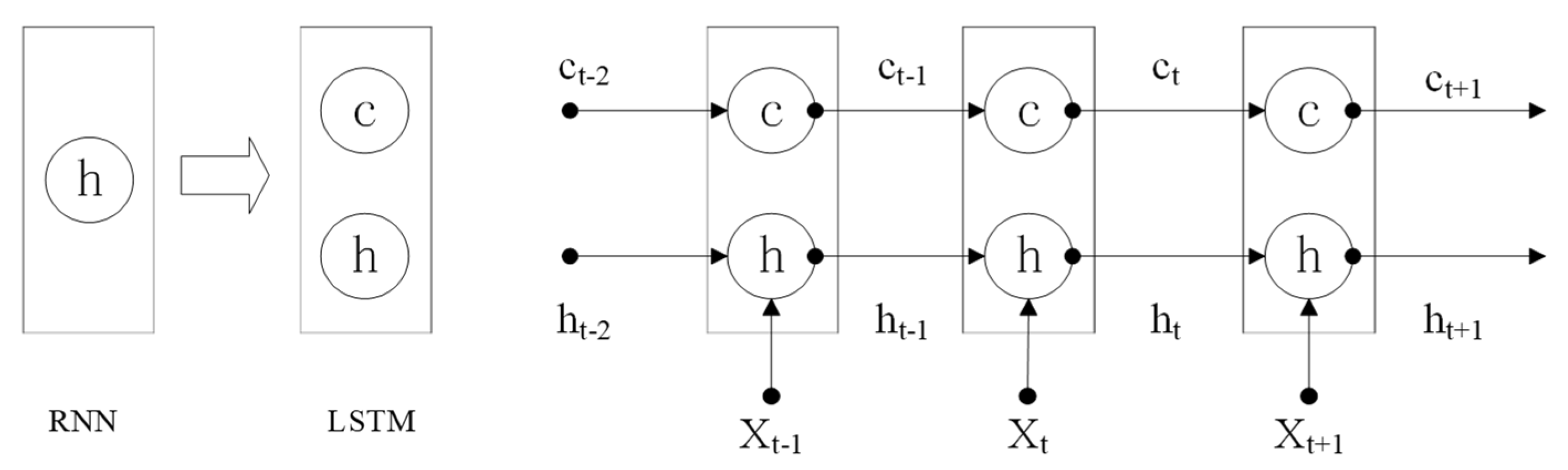
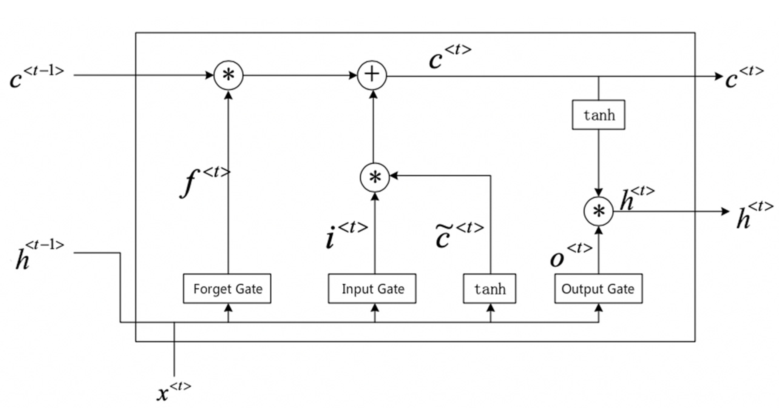
2. Approach
3. Dataset
3.1. Correlation Analysis
3.2. Data Completion
3.3. Standardized Processing
4. Experiment and Result
4.1. Evaluation
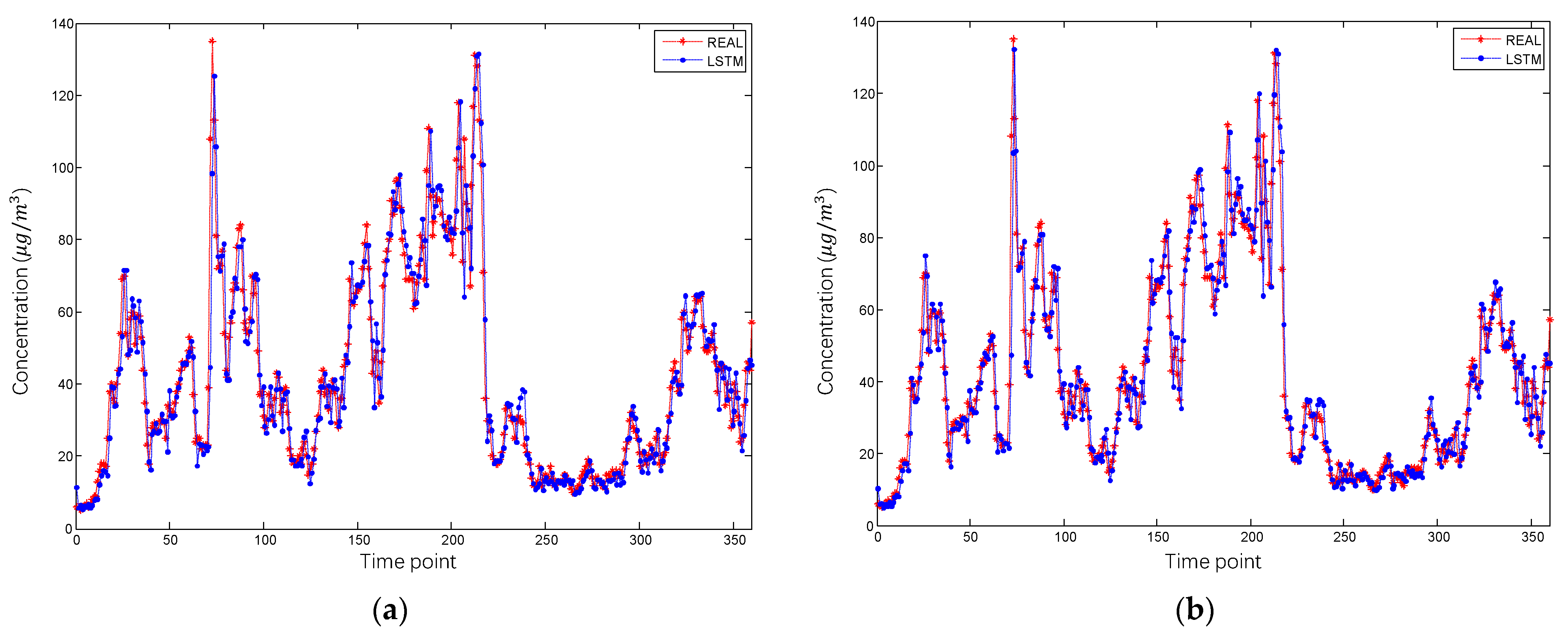
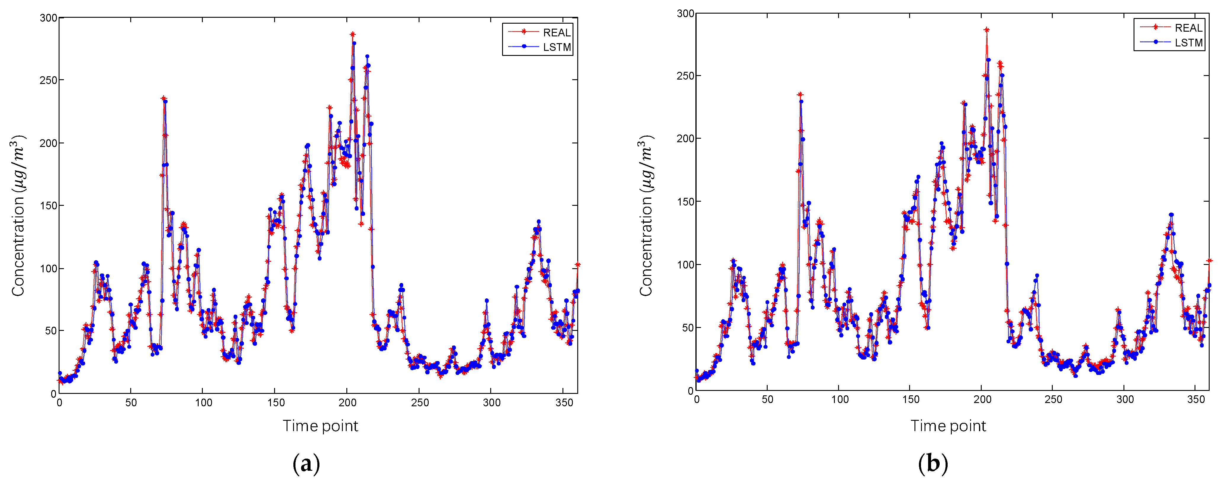
4.2. Result
5. Discussion
- We could feed the network with more data from areas adjacent to the target area whose haze concentration is what we want to predict. Haze is always a meteorological phenomenon, which indicates that the appearance of haze should be related to what is happening around the target area. For instance, if there is a signal of a powerful wind around the target area yet such signal is not included in our data, we could make a massive error because a powerful wind is likely to take pollutants away. Therefore, including data from adjacent areas could better fit the reality.
- A combination of different genres of deep learning models could be potentially helpful to increase accuracy. For example, we could consider that using a convolutional neural network to analyze a satellite photo could be helpful to give our sequential model a complete overall view of what is going to happen.
- Deep learning models always show their abilities when there are so many dimensions of the input. Thus, it is reasonable to add more parameters to the model to generate a prediction. In conclusion, adding extra dimensions should be considered as a way to improve accuracy.
- Since the GRU cell is generally a suitable replacement for the LSTM cell, since its complexity is lower yet the outcome remains much the same or even better, it is reasonable and worthy to use GRU to make predictions instead of LSTM. However, accuracy-wise speaking, LSTM is sufficient.
- Network Architecture Search (NAS), for instance, a Bayesian theory-based searching method [36], could help optimize our settings about the hyperparameters so that accuracy could be improved even further.
6. Conclusions
Author Contributions
Funding
Institutional Review Board Statement
Informed Consent Statement
Data Availability Statement
Conflicts of Interest
References
- Lirong, Y.; Zheng, W.; Yin, L.; Yin, Z.; Song, L.; Tian, X. Influence of Social-economic Activities on Air Pollutants in Beijing, China. Open Geosci. 2017, 9, 314–321. [Google Scholar] [CrossRef] [Green Version]
- Zheng, W.; Li, X.; Yin, L.; Wang, Y. Spatiotemporal heterogeneity of urban air pollution in China based on spatial analysis. Rend. Lincei 2016, 27, 351–356. [Google Scholar] [CrossRef]
- Zheng, W.; Li, X.; Yin, L.; Wang, Y. The retrieved urban LST in Beijing based on TM, HJ-1B and MODIS. Arab. J. Sci. Eng. 2016, 41, 2325–2332. [Google Scholar] [CrossRef]
- Li, X.; Lam, N.; Qiang, Y.; Li, K.; Yin, L.; Liu, S.; Zheng, W. Measuring County Resilience After the 2008 Wenchuan Earthquake. Int. J. Disaster Risk Sci. 2016, 7, 393–412. [Google Scholar] [CrossRef] [Green Version]
- Zheng, W.; Li, X.; Xie, J.; Yin, L.; Wang, Y. Impact of human activities on haze in Beijing based on grey relational analysis. Rend. Lincei 2015, 26, 187–192. [Google Scholar] [CrossRef]
- Hinton, G.E.; Salakhutdinov, R.R. Reducing the Dimensionality of Data with Neural Networks. Science 2006, 313, 504–507. [Google Scholar] [CrossRef] [Green Version]
- Zhang, J.; Liu, L.; Wang, Y.; Ren, Y.; Wang, X.; Shi, Z.; Zhang, D.; Che, H.; Zhao, H.; Liu, Y.; et al. Chemical composition, source, and process of urban aerosols during winter haze formation in Northeast China. Environ. Pollut. 2017, 231, 357–366. [Google Scholar] [CrossRef]
- Chaloulakou, A.; Kassomenos, P.; Spyrellis, N.; Demokritou, P.; Koutrakis, P. Measurements of PM10 and PM2.5 particle concentrations in Athens, Greece. Atmos. Environ. 2003, 37, 649–660. [Google Scholar] [CrossRef]
- Minguillón, M.; Querol, X.; Baltensperger, U.; Prévôt, A. Fine and coarse PM composition and sources in rural and urban sites in Switzerland: Local or regional pollution? Sci. Total Environ. 2012, 427, 191–202. [Google Scholar] [CrossRef]
- Ho, K.; Cao, J.; Lee, S.; Chan, C.K. Source apportionment of PM2. 5 in urban area of Hong Kong. J. Hazard. Mater. 2006, 138, 73–85. [Google Scholar] [CrossRef]
- Manly, B.F.; Alberto, J.A.N. Multivariate Statistical Methods: A Primer; Chapman and Hall/CRC: Boca Raton, FL, USA, 2016. [Google Scholar]
- Yin, L.; Li, X.; Zheng, W.; Yin, Z.; Song, L.; Ge, L.; Zeng, Q. Fractal dimension analysis for seismicity spatial and temporal distribution in the circum-Pacific seismic belt. J. Earth Syst. Sci. 2019, 128, 22. [Google Scholar] [CrossRef] [Green Version]
- Tang, Y.; Liu, S.; Li, X.; Fan, Y.; Deng, Y.; Liu, Y.; Yin, L. Earthquakes spatio–temporal distribution and fractal analysis in the Eurasian seismic belt. Rend. Lincei 2020, 31, 203–209. [Google Scholar] [CrossRef]
- Chen, X.; Yin, L.; Fan, Y.; Song, L.; Ji, T.; Liu, Y.; Tian, J.; Zheng, W. Temporal evolution characteristics of PM2.5 concentration based on continuous wavelet transform. Sci. Total Environ. 2020, 699, 134244. [Google Scholar] [CrossRef]
- Elbayoumi, M.; Ramli, N.A.; Yusof, N.F.F.M.; Bin Yahaya, A.S.; Al Madhoun, W.; Ul-Saufie, A.Z. Multivariate methods for indoor PM10 and PM2.5 modelling in naturally ventilated schools buildings. Atmos. Environ. 2014, 94, 11–21. [Google Scholar] [CrossRef]
- Li, T.; Hua, M.; Wu, X. A Hybrid CNN-LSTM Model for Forecasting Particulate Matter (PM2.5). IEEE Access 2020, 8, 26933–26940. [Google Scholar] [CrossRef]
- Zheng, W.; Li, X.; Lam, N.; Wang, X.; Liu, S.; Yu, X.; Sun, Z.; Yao, J. Applications of integrated geophysical method in archaeological surveys of the ancient Shu ruins. J. Archaeol. Sci. 2013, 40, 166–175. [Google Scholar] [CrossRef]
- Pérez, P.; Trier, A.; Reyes, J. Prediction of PM2.5 concentrations several hours in advance using neural networks in Santiago, Chile. Atmos. Environ. 2000, 34, 1189–1196. [Google Scholar] [CrossRef]
- Liu, S.; Wang, L.; Liu, H.; Su, H.; Li, X.; Zheng, W. Deriving Bathymetry from Optical Images with a Localized Neural Network Algorithm. IEEE Trans. Geosci. Remote Sens. 2018, 56, 5334–5342. [Google Scholar] [CrossRef]
- Deng, Y.; Tang, Y.; Yang, B.; Zheng, W.; Liu, S.; Liu, C. A Review of Bilateral Teleoperation Control Strategies with Soft Environment. In Proceedings of the 2021 6th IEEE International Conference on Advanced Robotics and Mechatronics (ICARM), Chongqing, China, 3–4 July 2021; pp. 459–464. [Google Scholar]
- Yin, L.; Wang, L.; Huang, W.; Liu, S.; Yang, B.; Zheng, W. Spatiotemporal Analysis of Haze in Beijing Based on the Multi-Convolution Model. Atmosphere 2021, 12, 1408. [Google Scholar] [CrossRef]
- Sherstinsky, A. Fundamentals of Recurrent Neural Network (RNN) and Long Short-Term Memory (LSTM) network. Phys. D Nonlinear Phenom. 2020, 404, 132306. [Google Scholar] [CrossRef] [Green Version]
- Zheng, W.; Liu, X.; Yin, L. Sentence Representation Method Based on Multi-Layer Semantic Network. Appl. Sci. 2021, 11, 1316. [Google Scholar] [CrossRef]
- Zheng, W.; Liu, X.; Ni, X.; Yin, L.; Yang, B. Improving Visual Reasoning through Semantic Representation. IEEE Access 2021, 9, 91476–91486. [Google Scholar] [CrossRef]
- Zheng, W.; Yin, L.; Chen, X.; Ma, Z.; Liu, S.; Yang, B. Knowledge base graph embedding module design for Visual question answering model. Pattern Recognit. 2021, 120, 108153. [Google Scholar] [CrossRef]
- Zheng, W.; Liu, X.; Yin, L. Research on image classification method based on improved multi-scale relational network. PeerJ Comput. Sci. 2021, 7, e613. [Google Scholar] [CrossRef]
- Li, Y.; Zheng, W.; Liu, X.; Mou, Y.; Yin, L.; Yang, B. Research and improvement of feature detection algorithm based on FAST. Rend. Lincei 2021, 1–15. [Google Scholar] [CrossRef]
- Qin, D.; Yu, J.; Zou, G.; Yong, R.; Zhao, Q.; Zhang, B. A novel combined prediction scheme based on CNN and LSTM for urban PM 2.5 concentration. IEEE Access 2019, 7, 20050–20059. [Google Scholar] [CrossRef]
- Tsai, Y.-T.; Zeng, Y.-R.; Chang, Y.-S. Air pollution forecasting using RNN with LSTM. In Proceedings of the 2018 IEEE 16th International Conference on Dependable, Autonomic and Secure Computing, 16th International Conference on Pervasive Intelligence and Computing, 4th International Conference on Big Data Intelligence and Computing and Cyber Science and Technology Congress (DASC/PiCom/DataCom/CyberSciTech), Athens, Greece, 12–15 August 2018; pp. 1074–1079. [Google Scholar]
- Bai, Y.; Zeng, B.; Li, C.; Zhang, J. An ensemble long short-term memory neural network for hourly PM2.5 concentration forecasting. Chemosphere 2019, 222, 286–294. [Google Scholar] [CrossRef] [PubMed]
- Tang, Y.; Liu, S.; Deng, Y.; Zhang, Y.; Yin, L.; Zheng, W. An improved method for soft tissue modeling. Biomed. Signal Process. Control. 2021, 65, 102367. [Google Scholar] [CrossRef]
- Ma, Z.; Zheng, W.; Chen, X.; Yin, L. Joint embedding VQA model based on dynamic word vector. PeerJ Comput. Sci. 2021, 7, e353. [Google Scholar] [CrossRef] [PubMed]
- Zhang, Z.; Tian, J.; Huang, W.; Yin, L.; Zheng, W.; Liu, S. A Haze Prediction Method Based on One-Dimensional Convolutional Neural Network. Atmosphere 2021, 12, 1327. [Google Scholar] [CrossRef]
- Gers, F.A.; Schmidhuber, J.; Cummins, F.A. Learning to Forget: Continual Prediction with LSTM. Neural Comput. 2000, 12, 2451–2471. [Google Scholar] [CrossRef] [PubMed]
- Keane, R.D.; Adrian, R.J. Theory of cross-correlation analysis of PIV images. Flow Turbul. Combust. 1992, 49, 191–215. [Google Scholar] [CrossRef]
- Snoek, J.; Larochelle, H.; Adams, R.P. Practical bayesian optimization of machine learning algorithms. Adv. Neural Inf. Process. Syst. 2012, 25, 2951–2959. [Google Scholar]


| Correlation Coefficient | Highest Temperature | Lowest Temperature | Humidity | Wind Power | O3 | CO | NO2 | PM10 | SO2 |
|---|---|---|---|---|---|---|---|---|---|
| winter | 0.29 | −0.01 | −0.25 | −0.35 | −0.13 | 0.49 | 0.54 | 0.79 | 0.48 |
| summer | 0.38 | −0.05 | −0.22 | −0.38 | −0.56 | 0.67 | 0.38 | 0.95 | 0.39 |
| Level | 1 | 2 | 3 | 4 | 5 | 6 |
|---|---|---|---|---|---|---|
| Level range (μg/m3) | 0–35 | 36–75 | 76–115 | 116–150 | 151–250 | >250 |
| Hidden Layers | Neuron Distribution | PM2.5 RMSE μg/m3 | Excellent | Acceptable | Unacceptable |
|---|---|---|---|---|---|
| 1 | 10 | 10.95 | 80.83% | 18.89% | 0.28% |
| 2 | 10 9 | 9.72 | 81.67% | 18.33% | 0.00% |
| 3 | 10 9 8 | 8.81 | 84.44% | 15.56% | 0.00% |
| 4 | 10 9 8 7 | 8.41 | 83.89% | 16.11% | 0.00% |
| 5 | 10 9 8 7 6 | 8.18 | 85.28% | 14.72% | 0.00% |
| 6 | 10 9 8 7 6 5 | 8.31 | 84.72% | 15.28% | 0.00% |
| 7 | 10 9 8 7 6 5 4 | 8.11 | 86.39% | 13.61% | 0.00% |
| 8 | 10 9 8 7 6 5 4 3 | 8.23 | 85.56% | 14.44% | 0.00% |
| Hidden Layers | Neuron Distribution | PM10 RMSE μg/m3 | Excellent | Acceptable | Unacceptable |
|---|---|---|---|---|---|
| 1 | 10 | 18.95 | 73.89% | 25.28% | 0.83% |
| 2 | 10 9 | 17.02 | 78.61% | 21.11% | 0.28% |
| 3 | 10 9 8 | 16.66 | 79.72% | 20.00% | 0.28% |
| 4 | 10 9 8 7 | 16.05 | 80.56% | 19.17% | 0.28% |
| 5 | 10 9 8 7 6 | 15.40 | 81.11% | 18.89% | 0.00% |
| 6 | 10 9 8 7 6 5 | 15.48 | 81.11% | 18.89% | 0.00% |
| 7 | 10 9 8 7 6 5 4 | 15.41 | 81.67% | 18.33% | 0.00% |
| 8 | 10 9 8 7 6 5 4 3 | 15.40 | 81.39% | 18.61% | 0.00% |
Publisher’s Note: MDPI stays neutral with regard to jurisdictional claims in published maps and institutional affiliations. |
© 2021 by the authors. Licensee MDPI, Basel, Switzerland. This article is an open access article distributed under the terms and conditions of the Creative Commons Attribution (CC BY) license (https://creativecommons.org/licenses/by/4.0/).
Share and Cite
Wu, X.; Liu, Z.; Yin, L.; Zheng, W.; Song, L.; Tian, J.; Yang, B.; Liu, S. A Haze Prediction Model in Chengdu Based on LSTM. Atmosphere 2021, 12, 1479. https://doi.org/10.3390/atmos12111479
Wu X, Liu Z, Yin L, Zheng W, Song L, Tian J, Yang B, Liu S. A Haze Prediction Model in Chengdu Based on LSTM. Atmosphere. 2021; 12(11):1479. https://doi.org/10.3390/atmos12111479
Chicago/Turabian StyleWu, Xinyi, Zhixin Liu, Lirong Yin, Wenfeng Zheng, Lihong Song, Jiawei Tian, Bo Yang, and Shan Liu. 2021. "A Haze Prediction Model in Chengdu Based on LSTM" Atmosphere 12, no. 11: 1479. https://doi.org/10.3390/atmos12111479