Polar Amplification and Ice Free Conditions under 1.5, 2 and 3 °C of Global Warming as Simulated by CMIP5 and CMIP6 Models

Simple Summary

Polar regions are more sensitive to the increase in atmospheric CO₂ concentration than the rest of the world. This phenomenon is known as the Polar Amplification and is related to many nonlinear, complex coupled ocean-atmosphere processes with effects beyond high latitudes. Aiming to account for the Polar Amplification, this study used global climate simulations to investigate the effects of three different global warming thresholds (1.5, 2 and 3 °C) in the warming and sea ice conditions of both poles. Our results shown high climate sensitivity in the Arctic and Antarctica as a response to the increase in atmospheric CO₂ concentration. The warming signal is not symmetric in the two poles: the Arctic warms faster than Antarctica in all climate scenarios. Global warming crosses the minimum (maximum) future scenarios thresholds of +1.5 °C (+3 °C) around 2024 (2063). The equivalent Arctic (Antarctic) warming for these years is 3.6 (1.5) °C and (3.2) 6.6 °C, respectively. Although limited, Global Climate models used here are important tools to help on better understand the projected effects of climate change in high latitudes.

Abstract

One of the most visible signs of global warming is the fast change in the polar regions. The increase in Arctic temperatures, for instance, is almost twice as large as the global average in recent decades. This phenomenon is known as the Arctic Amplification and reflects several mutually supporting processes. An equivalent albeit less studied phenomenon occurs in Antarctica. Here, we used numerical climate simulations obtained from CMIP5 and CMIP6 to investigate the effects of +1.5, 2 and 3 °C warming thresholds for sea ice changes and polar amplification. Our results show robust patterns of near-surface air-temperature response to global warming at high latitudes. The year in which the average air temperatures brought from CMIP5 and CMIP6 models rises by 1.5 °C is 2024. An average rise of 2 °C (3 °C) global warming occurs in 2042 (2063). The equivalent warming at northern (southern) high latitudes under scenarios of 1.5 °C global warming is about 3 °C (1.8 °C). In scenarios of 3 °C global warming, the equivalent warming in the Arctic (Antarctica) is close to 7 °C (3.5 °C). Ice-free conditions are found in all warming thresholds for both the Arctic and Antarctica, especially from the year 2030 onwards.

1. Introduction

The Paris Agreement of the United Nations Framework Convention on Climate Change [1] in December 2015 proposed an aspirational goal to stabilize the mean air temperature to well below 2 °C and limited to 1.5 °C above the pre-industrial levels through sustained efforts [1]. In scientific research, the Paris Agreement warming thresholds have been widely used to better understand the complex and nonlinear effects of Climate Change on a wide range of environmental processes [2,3,4,5,6]. Numerous publications and reports, including the reports from the Intergovernmental Panel on Climate Change (IPCC), had discussed the impacts and risks of global warming under 1.5 °C and 2 °C targets, pointing to the high sensitivity of polar regions to the anthropogenic forcing [7,8,9].

Polar regions, owing to the presence of ice (sea ice, continental ice and permafrost), are more sensitive to climate change than the rest of the world [10,11]. One of the most visible aspects of the recent climate change, for instance, is the fast shrinking of the Arctic Sea ice cover resulting from the enhanced warming due to polar amplification [10,11]. Polar amplification (PA) refers to the ratio between high latitudes warming with respect to tropical warming and is recognized as an inherent characteristic of the global climate system [10,11,12]. The causes of PA, especially in southern latitudes, are still unclear and debated [10,12,13]. Indeed, different conclusions have been drawn to explain the coupled mechanism involved in the process, the ocean-atmosphere feedback mechanisms and whether the poleward, atmospheric heat transport may also be a key mechanism to understand polar warming [12,14,15]. Most of these studies use numerical climate simulations with radiative forcing of greenhouse gases (GHG) as the main tool [10,12,15]. One key aspect of this debate to understand the physical mechanisms underlying polar amplification is the difference between the methods adopted. For instance: [16], using climate simulations with prescribed changes in the sea surface temperatures (SST) and sea ice cover, suggested that the enhanced Arctic near-surface warming is due to Arctic Sea ice loss associated with local SST changes. Similarly, many other studies suggest that the sea ice-albedo feedback is the main mechanism explaining the Arctic PA [11,17]. However, studies using both observations and numerical simulations suggest that the sea ice-albedo feedback mechanism cannot alone explain the Arctic PA [15,18,19], and using a coupled model with simulations driven by CO₂ forcing, found that the largest contribution to polar warming in northern high latitudes comes from temperature feedback (as the Earth’s surface warms, more energy is radiated back to space in lower latitudes, compared with the Arctic). The understanding of the physical coupled processes underlying the PA plays a key role to offer confidence and also for constraining model projections of Arctic and Antarctic climate change.

Although there are many issues under debate regarding the driving mechanism involved in Arctic amplification, both observations and climate simulations indicate an enhanced warming associated with drastic sea ice melting over the past decades, which is projected to continue as response to the atmospheric CO₂ increase [17,20]. In contrast, the Antarctic Sea ice area, except for the Bellingshausen-Amundsen sector, has shown a slight increase over recent decades [21,22]. Many mechanisms have been proposed to explain the observed positive Antarctic Sea Ice Extent (SIE) trend; however, we still lack conclusive answers. Previous studies suggested the importance of mechanisms such as the wind variability, the ozone depletion, Antarctica’s natural variability and the effects of increasing freshwater input from Antarctica’s ice sheet into the ocean [23,24,25,26,27]. Furthermore, the inability of climate models to represent the observed positive trends in Antarctic SIE represents a key challenge for the scientific community, even for the latest CMIP6 dataset [28,29,30,31,32]. The Antarctic PA is expected in the future as response to CO₂ increases, probably delayed in relation to the Arctic PA. This is due to the strong heat absorption of atmospheric heat by the water in the Southern Ocean [10,25].

According to [33], the asymmetry in the PA between the two poles is related to the thermal inertia and the coupled ocean-atmosphere processes involved. While at the northern high latitudes, the amplified warming signal is associated with a positive snow-albedo and sea ice-albedo feedback, at the southern high latitudes, the warming is related to a combination of ozone depletion and changes in the wind pattern.

With the projected climate change for polar regions that has captured scientific and public attention over the last decade, a key scientific and open issue is assessing the time when summer ice-free conditions will be reached in the Arctic. It is known that the impacts of these changes extend well beyond the Arctic region [34,35,36,37].

In the present paper, we investigate the changes in the atmosphere, air temperature as well as the Arctic and Antarctic SIE for both past and future CMIP5 and CMIP6 scenarios. We aim to contribute to our understanding of climate change impacts under the global warming target specified by the Paris Agreement using 1.5, 2 and 3 °C global warming. These scenarios were chosen due to their political and environmental relevance [38]. Our analysis has two overarching aims: (1) we want to evaluate the ability of CMIP5 and CMIP6 to simulate the SIE seasonal cycle in relation to observations and (2) we want to understand the impact of different thresholds of warming on PA and SIE for the Arctic and Antarctica. The paper is structured as follows: first, we present the data sources in Section 2. In Section 3, we examine the SIE seasonal cycle, comparing CMIP5 and CMIP6 historical simulations with satellite data. Furthermore, we investigate future changes for the Arctic and Antarctica using the Representative Concentration Pathway RCP8.5 and the Shared Socioeconomic Pathways SSP585 scenarios [39,40]. We then discuss our results and indicate the consequences of the 1.5, 2 and 3 °C global warming levels for PA and sea ice changes, including the occurrence of summer ice-free conditions. Finally, in Section 4, we present our conclusions and lay out our recommendations for future work.

2. Materials and Methods

Climate Simulations

The Coupled Model Intercomparison Projects (CMIP) are an international effort of the scientific community using different climate models around the world to provide multi-model simulations at the global scale, with a complete representation of external forcing and a wide set of scenarios aimed to provide a useful tool to better understand the Earth’s past and future climate changes [39,40].

The present study used three numerical experiments taken from CMIP5 and CMIP6: (i) Historical, (ii) RCP8.5 and (iii) SSP585. The CMIP5 future scenarios are defined by the Representative Concentration Pathways (RCPs), and each RCP defines a specific emissions trajectory and subsequent radiative forcing. The radiative forcing value in the year 2100 relative to pre-industrial values is 8.5 W·m⁻² for RCP8.5, which includes the period from 2006 to 2100. The equivalent scenario to compare RCP85 in the Shared Socioeconomic Pathways is the SSP585, which includes the period from 2015 to 2100. The atmospheric CO₂ concentration in the year 2100 is 1200 ppm in both RCP8.5 and SSP585 scenarios. The simulations of the historical experiment for the CMIP5 are integrated over 156 years, starting in 1850 until 2005, forced by the observed historical series of the CO₂ concentration of the same period. On the other hand, the historical experiment of CMIP6 was started in 1850 until 2014, totaling 165 years. Furthermore, all models need to spin-up before starting the piControl, the Historical and the Scenarios experiments. The complete description of the numerical experiments design is found in [39] for CMIP5 and in [40,41] for CMIP6.

Here, we used near-surface temperature and sea ice concentration to calculate the SIE from 49 CMIP climate models’ outputs (refer to the Supplementary Materials). SIE is measured as the total area of all grid cells that has a sea ice concentration exceeding 15%. First, we aimed to understand the ability of CMIP simulations to represent the sea ice seasonal cycle during the period 1980–2005 (CMIP5) and 1980–2014 (CMIP6) using the historical numerical experiments. Second, we aimed to calculate the Arctic and Antarctic PA.

PA is often characterized as the ratio of high latitudes and surface air temperature changes compared to global air temperature change [10,33]. For the past, we used air temperatures from the European Center for Medium-Range Weather Forecast (ECMWF) ERA-5 reanalysis (available online at www.ecmwf.int (accessed on 5 September 2021)). We used monthly updates for the 2010–2020 period relative to the 1980–1990 period, providing a measure of the climate sensitivity in high latitudes. For future scenarios, we used the period related to initial timing of 1.5, 2 and 3 °C global warming for each climate model.

In order to evaluate the sea ice model’s performance, we used the satellite data set from the Scanning Multichannel Microwave Radiometer (SSMR) on the Nimbus-7 satellite and from the Special Sensor Microwave/Imager SSM/I on the Defense Meteorological Satellite Program’s (DMSP), available in National Snow & Ice Data Center (NSIDC) [42].

3. Results and Discussion

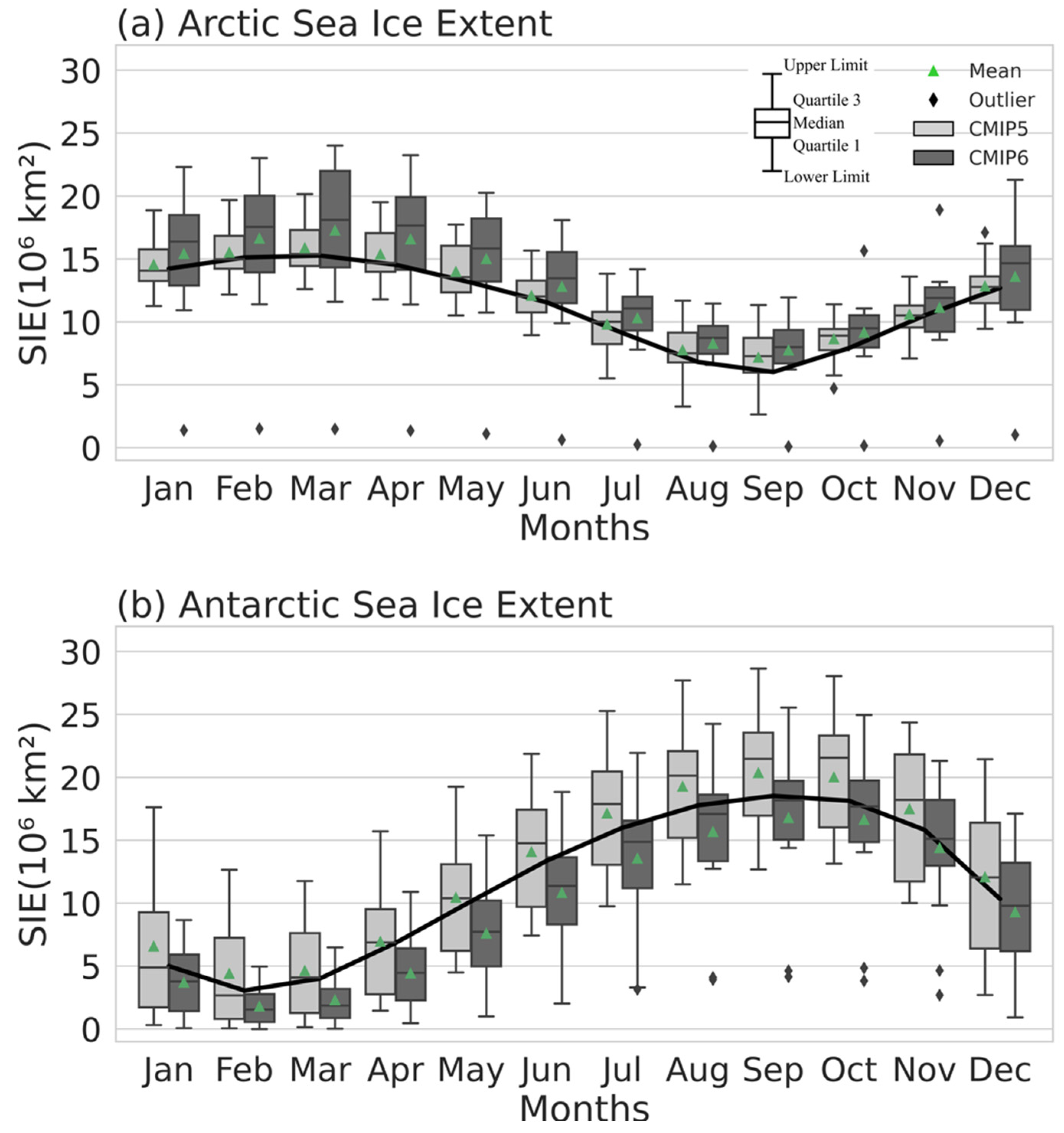
3.1. Sea Ice Seasonal Cycle

The sea ice seasonal cycle is closely related to the near-surface air temperature, heat fluxes and ocean heat content and can strongly affect the ocean and atmosphere circulation [10,43]. We start with an analysis of seasonal SIE simulated by CMIP5 (CMIP6) over the period from 1980–2005 (1980–2014). Figure 1 shows the performance of CMIP models to simulate the melt-freeze transitions by the SIE seasonal cycle for the Arctic and Antarctica. We found a large spread for SIE conditions on both CMIP simulations for all months, albeit this variance is relatively larger in the cold (northern and southern hemisphere) seasons. For the northern hemisphere (Figure 1a), in the period of maximum SIE (March), the mean SIE simulated by CMIP5 (CMIP6) ranged from around 13 × 10⁶ km² (11 × 10⁶ km²) to more than 19 × 10⁶ km² (23 × 10⁶ km²), thus corroborating the observational estimate of 15 × 10⁶ km² for the same month. On average, March SIEs from CMIP5 and CMIP6 were close to 15.2 × 10⁶ km² and 18 × 10⁶ km², respectively. Some CMIP6 models, however, presented very high SIEs for March in the Arctic (more than 21 × 10⁶ km²), causing an overestimation of SIE with respect to observational data. This is consistent with results presented by [28]. Refs. [43,44] suggest that a positive SIE bias is related to the tendency of climate models to underestimate the amount of longwave (LW) radiation reemitted back to the Earth’s surface in the cold season. During winter, the amount of radiation is low, and the ability of the clouds to reemit LW to the surface provides a positive radiative effect on the surface energy.

In September, the mean SIE in the Arctic simulated by CMIP5 (CMIP6) ranged from around 2.5 × 10⁶ km² (6.4 × 10⁶ km²) to more than 12 × 10⁶ km² (12.5 × 10⁶ km²), again corroborating the monthly mean satellite observation of 6 × 10⁶ km². On average, the Arctic SIE in September, as estimated from CMIP5 and CMIP6, is about 7 × 10⁶ km² and 7.5 × 10⁶ km², respectively. This is consistent with [32,45]. According to [28], CMIP6 models are not able to reproduce the summer tendencies after the year 2000, including the Arctic’s rapidly shrinking sea ice cover, especially in the regions of Kara and Barents seas. Ref. [28] reports that the reliability of future scenarios in CMIP6 depends on the models’ ability to represent the past. We also need to understand the ocean-atmosphere coupled processes that are responsible for the large spread among CMIP6 models. At this point, it is important to consider the sources of the systematic errors in climate simulations that result in inefficiency to reproduce sea ice changes, as well as the process involved. According to [44], the annual amplitude of sea ice cover inversely depends on the sea ice-albedo that consequently determines the poor representation of the Arctic Sea ice-albedo feedback and cloud radiation in the CMIP5 models. The correct representation of the albedo by the ocean models offers improvements in our knowledge about the surface-atmosphere feedback processes and in the surface radiation budget. Then, a better performance of climate models to represent SIE may be achieved. As a consequence, we may also get more robustness in future scenarios, especially in relation to current Arctic transitions to ice-free summer conditions, considered nowadays a hot topic of research.

For the southern hemisphere (Figure 1b), all models were able to capture the mean SIE seasonal cycle, although quantitatively there is a large intermodel spread, especially among CMIP5 models. During February, the period of SIE minimum in the southern hemisphere, the mean SIE simulated by CMIP5 (CMIP6) ranged from around 1.2 × 10⁶ km² (1 × 10⁶ km²) to more than 12 × 10⁶ km² (5 × 10⁶ km²), thus including the observational measure of 3 × 10⁶ km². During the period of SIE minimum in the southern hemisphere, on average, both CMIP5 and CMIP6 tend to underestimate the SIE in comparison to observations. Even so, the CMIP6 intermodel spread is relatively low, indicating a best performance. According to [29], the CMIP6 presents improvements in the representation of then real sea ice extent as well as a better localization of the sea ice. Ref. [28] reported that the light but significant positive trend in Antarctica’s SIE is not captured in CMIP6. The authors report that this was already an issue in CMIP5 outputs, suggesting that, even with improvements, the CMIP models are still unable to reproduce the observed Antarctic Sea ice.

Our results show that the Arctic SIE is better represented than the Antarctic SIE, corroborating the results of [28,30]. According to [23,31], the main problem of using climate models in Antarctica is related to their inability to capture the observed increase in sea ice cover. Refs. [24,26,27] have demonstrated the importance of Antarctica ice sheet dynamics on simulated sea ice, disregarded in most CMIP models. According to [27], the increase in ocean temperatures results in basal ice-shelf melt, freshening the surface waters around Antarctica and thus triggering an increase of SIE.

Changes in sea ice extent have become a central focus of scientific and governments’ discussions due to its high sensitivity to changes and its impact on the ocean and atmospheric circulation. A precise assessment of the performance of models to simulate sea ice is essential to determine the models’ ability to represent future scenarios and to improve the climate models themselves.

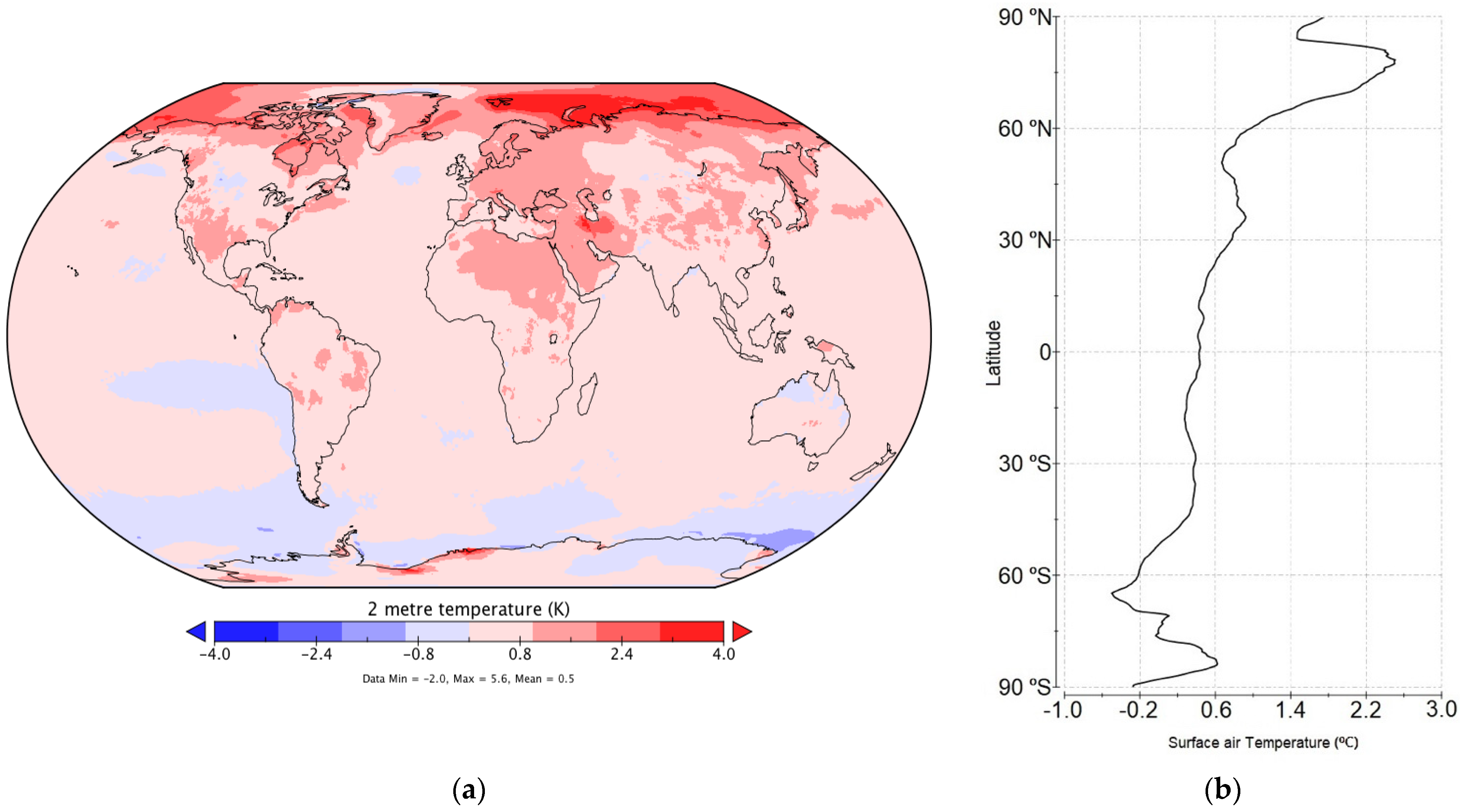
3.2. Polar Amplification

Figure 2 shows the measure of PA taken from long-term observations of the near-surface air temperature for the 2010–2020 period relative to the 1980–1990 period. The figure also presents the zonal mean of the near-surface temperature for 2010–2020 relative to 1980–1990. The results emphasize the strong climate sensitivity of the polar regions to the global warming. The Arctic region is rapidly warming at a rate of at least twice as fast as the global average. The observed warming of the Southern Ocean and the Antarctic ice sheet is generally modest in relation to the Arctic’s warming, but t is still not negligible. The Antarctic Peninsula and the Weddell Sea region, for example, warmed at more than twice the rate of the entire globe. The asymmetry between the high latitudes of southern and northern hemispheres is partly caused by the smaller area covered by the Arctic Ocean with respect to the Southern Ocean. As the ocean’s area and volume are directly related to the (incoming) short wave absorption, the smaller area covered by the Arctic Ocean induces a smaller thermal inertia in the northern hemisphere [13,33].

In the northern hemisphere, regions close to the Kara and Barents seas registered robust warming patterns above 3.5 °C in the period analyzed here. This region produces dense waters that are one of the main sources of Arctic Intermediate Water, an important driver of the Arctic thermohaline circulation.

Ref. [33] suggested that the Arctic amplification is closely related to sea ice loss. According to [46], the Arctic Ocean in general and the Barents Sea in particular had experienced dramatic loss of sea ice as a result of the Barents Sea ice cooling machine being changed to a less efficient cooling due to a warmer Atlantic inflow, the consequent sea ice loss and then to more ocean heat loss. Ref. [47], using CO₂ forced numerical experiments, showed that the Arctic amplification develops rapidly and before any significant sea ice loss. This occurs owing to positive lapse rate feedback, that is, the sea ice shrinking is not necessary to produce polar enhanced warming, although it contributes significantly to the process. Several recent studies proposed different mechanisms to explain the fast sea ice loss, the emergence of the Arctic amplification and its effect on the climate system [12,47,48]. The causes of the Arctic amplification have long been attributed to the local forcing and surface-atmosphere feedback mechanisms [12,15] as well as to changes in the poleward heat transport by the ocean and the atmosphere [14,49]. However, the underlying causes of the whole phenomenon are not yet fully understood.

At this point, it is important to consider how the spatial variability of the atmospheric CO₂ concentration (ACC) is treated in climate simulations. Most CMIP simulations consider the ACC as globally homogeneous [50]. However, the reality is that the ACC due to human CO₂ emission varies widely, with high (low) values over the mid latitudes of the northern (southern) hemisphere. Recent studies reported that the heterogeneous spatial distribution of the ACC may induce different climate effects, and the use of more realistic input data may produce more realistic global climate simulations [12,49,51]. According to [12], the degree of polar amplification depends strongly on the location of the CO₂ forcing. The authors also report that the contribution of remote (extra-polar) forcing to the polar amplification is modest when we consider the real ACC spatial distribution. We suggest that, especially for southern latitudes, the inability of climate models to represent the heterogeneity of the ACC’s spatial distribution, added to the lack of a southern hemisphere ice sheet component in the CMIP models, culminate in an important source of error in both the polar amplification estimate and the sea ice representation in the southern hemisphere.

This is relevant considering the expected twenty-first century warming and the projected ice-free conditions for both the Arctic and Antarctica, further studied in this paper. Ref. [52] points out the lesser resilience of the Arctic region over the last decades. The fast decrease in SIE and sea ice thickness over the last decades led to an Arctic climate system more vulnerable to short-term climate fluctuations and a revisit to the concept of abrupt climate change [53]. The extreme weather and climate events linked with abrupt changes in high latitudes have attracted considerable scientific and international media interest over the last decade. The 2020 Siberian heat wave (which sets a record for the highest air temperature registered in the Arctic Circle of 38 °C), reported by [52], reinforced the importance to better understand the high latitudes climate sensitivity and effects.

Figure 2 also corroborates with the results presented by [54,55]. According to the authors, the central areas of Western Antarctica are one of the fastest warming regions on Earth, with a temperature increase of 2.4 °C with respect to pre-industrial levels. Ref. [55] pointed out that while the ground station records located in the Antarctic Peninsula do not indicate a ubiquitous polar amplification, the recent rapid regional warming might be indeed the regional amplification of the global warming.

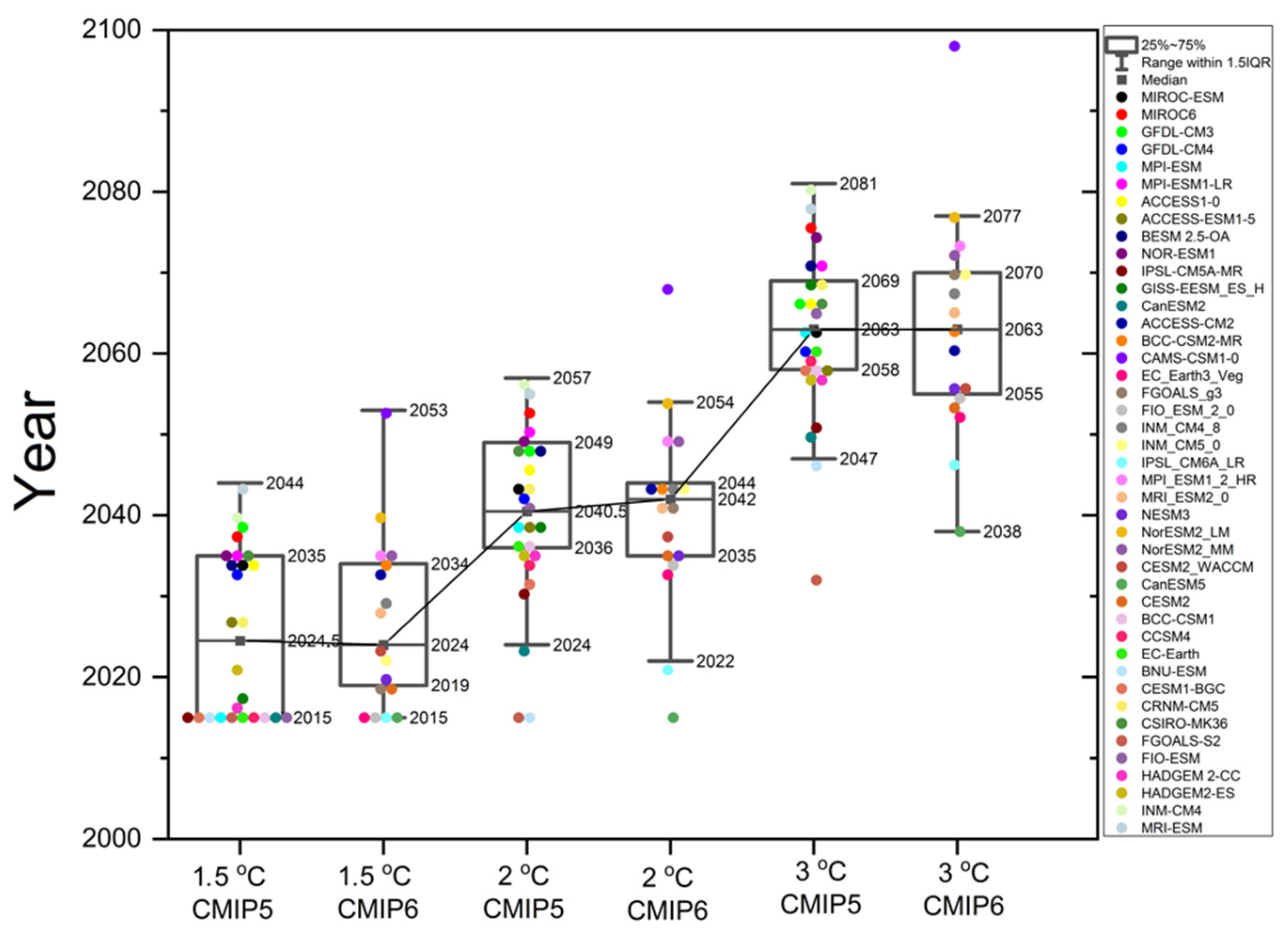
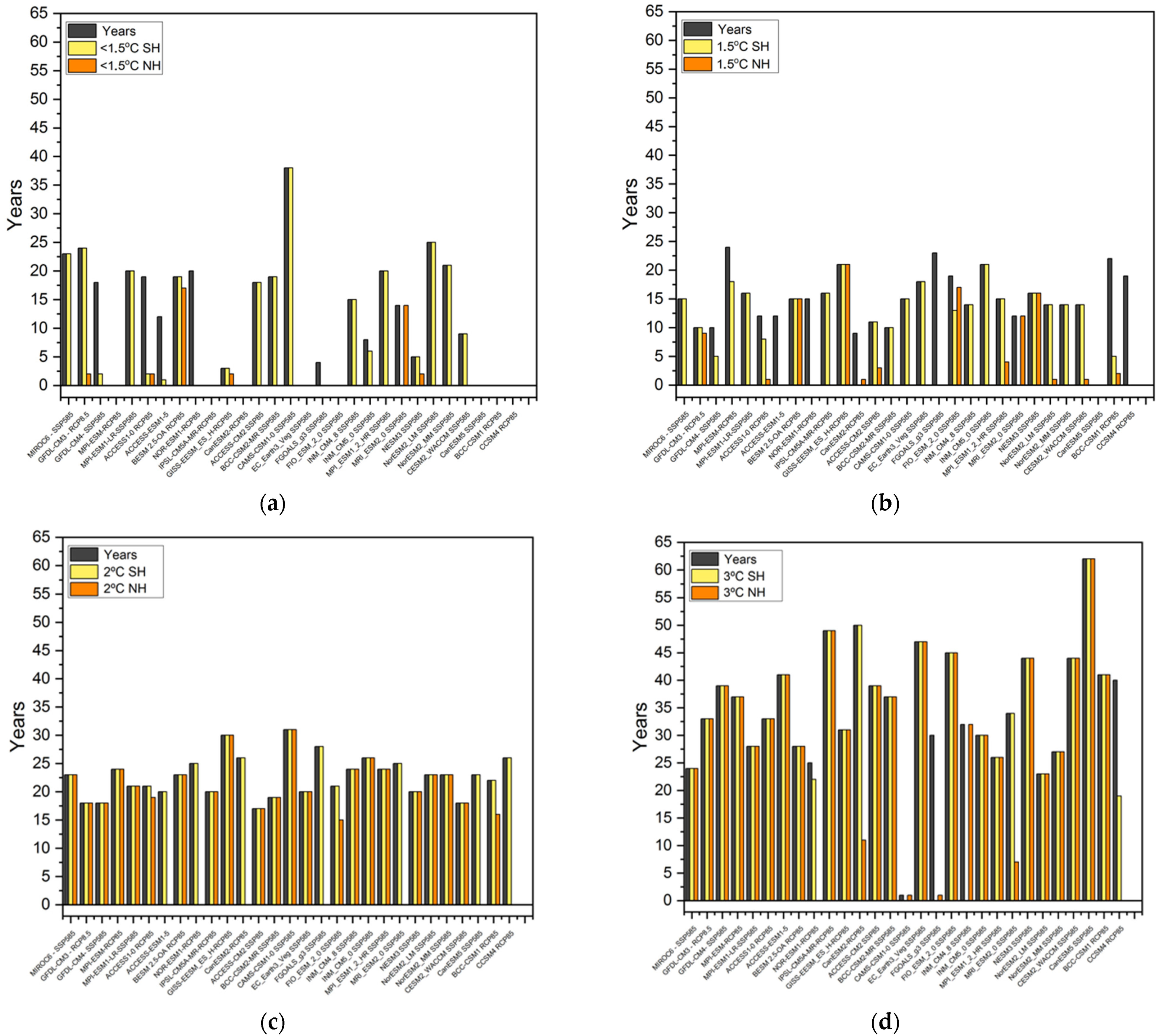
3.3. Initial Timing of 1.5, 2 and 3 °C Mean Global Warming

The effects of climate change at +1.5 °C, +2.0 °C and +3.0 °C of global warming above pre-industrial levels are investigated in this section. We specifically focus on the signature of polar amplification and sea ice extent changes. This approach has been widely taken on different perspectives, especially aiming to identify the most vulnerable regions in the planet to climate change. Even so, only few studies are available so far for describing the effects of climate change in polar regions [56,57,58,59]. Studying the effects of climate change in polar regions is also relevant in the political context, helping in identifying the benefits of potential mitigation efforts.

First, in order to assess the polar climate changes connected to a global mean temperature increase considering the Paris Agreement thresholds, we searched for the time frames when CMIP5 and CMIP6 global averaged, near-surface level air temperatures cross the limit of +1.5 °C, 2.0 °C and 3.0 °C global warming with respect to pre-industrial, global averaged levels as seen in each of the respective models.

Results are presented in Figure 3. The central 50% intermodal range (25–75%), the median, and upper and lower boundaries in the CMIP models are indicated by the box plot in Figure 3. Global warming crosses the +1.5 °C limit in the year 2024 in both CMIP5 and CMIP6 projections. This is alarming, for the world is likely to exceed the +1.5 °C threshold in the short range of the next coming years. This result corroborates with [56] even for the more optimistic scenario. The CMIP5 (CMIP6) interquartile range from the year 2015 to 2035 (2019 to 2034) and the upper boundary is found in 2044 (2053). We identified that MRI-ESM (RCP 8.5) and CAMS-CSM1-0 (SSP585) were the models that took the longest to reach the +1.5 °C global warming, which occurred in the years 2044 and 2053, respectively (Figure 3). The initial timing when the global warming crosses the +2.0 °C threshold was found close to 2040 (2042) for CMIP5 (CMIP6) projections, with interquartile ranging from the year 2036 to 2049 (2035 to 2044), and the upper boundary is close to 2057 (2054). The threshold +3.0 °C global warming was projected for the year 2063 for both CMIP5 and CMIP6 simulations. The +3 °C threshold interquartile ranges of CMIP5 (CMIP6) are 2058 to 2069 (2055 to 2070).

The models that took the longest to reach the temperature target of +2.0 °C were, as expected, the same models previously described here: MRI-ESM (RCP8.5), CAMS- CSM1-0 (SSP585) plus, additionally, INM-CM4 (RCP8.5) and NorESM2-LM (SSP585) in the years 2055, 2068, 2057 and 2054 (Figure 3). Figure 3 indicates that the models reaching fastest the target of +3.0 °C global warming are FGOALS-s2 (RCP8.5) and CanESM5 (SSP585) in the forthcoming years of 2032 and 2038. Both models also reach the 1.5 °C and 2.0 °C global warming threshold earlier in comparison to other CMIP models.

The global warming median values, for all temperature targets considered here, are similar to each other when comparing CMIP5 and CMP6 simulations. However, the effects of these warming thresholds are expected to vary widely in different regions of the planet, as well varying greatly inside each model. These results are in agreement with previous results presented by [56,59,60].

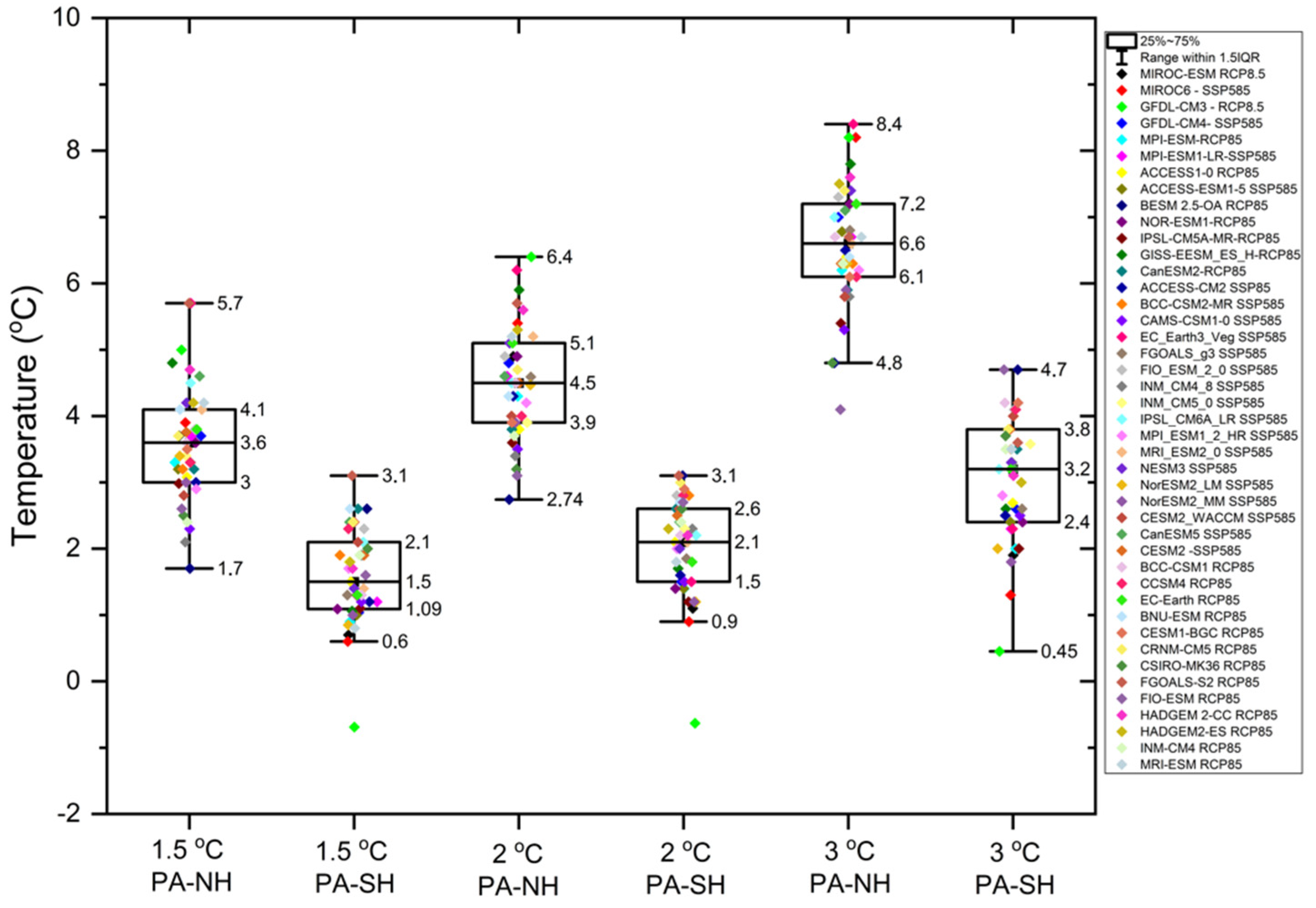
3.4. Polar Amplification under 1.5, 2 and 3 °C Mean Global Warming

In this session, we investigate the PA of climate models considering the temperature threshold of +1.5 °C, 2.0 °C and 3.0 °C global warming. To isolate the PA signal of global warming, we consider latitudes above 60° N and 60° S, following the methodology widely used in previous studies [10,12,33]. In Figure 4, the box plot indicates the central 50% intermodel range (25–75%), the median and upper and lower boundaries of each CMIP model for PA of climate change. Figure 5 shows the warming rate caused by the PA with respect to the Earth’s average global warming for the period when models reach the threshold of +1.5 °C, 2.0 °C and 3.0 °C global warming (previously calculated—Figure 4); thus, we have a measure of how amplified the polar regions were in relation to global warming. For example, a warming rate of 2 indicates that the polar warming (amplification) in the poles is two times larger than the global warming average.

Figure 4 and Figure 5 show the enhanced warming at high latitudes compared with the overall Earth’s global warming (Figure 3) considering the thresholds of +1.5 °C, 2.0 °C and 3.0 °C global warming. Clearly, this warming is not symmetric, with higher values in the high latitudes of the northern hemisphere. Results seen in Figure 4 show that for the +1.5 °C (+2.0 °C) Paris Agreement target, the simulated median warming at northern hemisphere high latitudes was 3.6 °C (4.5 °C), with interquartile ranging from 3.0 °C to 4.1 °C (3.9 to 5.1 °C) and the upper boundaries close to 5.7 °C (6.4 °C). Considering the +3.0 °C global warming threshold, the simulated median warming was close to 6.6 °C, and the interquartile ranged from 6.1 °C to 7.2 °C. The warming rate simulations shown in Figure 5, for all targets (+1.5 °C, 2.0 °C and 3.0 °C) are similar, presenting values more than twice as large as the global average (2.4, 2.3 and 2.2 times, respectively).

For the southern hemisphere high latitudes, the median warming simulated for the +1.5 °C (+2 °C) Paris Agreement target was 1.5 °C (2.1 °C), with interquartile range from 1.9 °C to 2.1 °C (1.5 °C to 2.6°C). The lower boundary was close to 0.6 °C (0.9 °C), that is, simulated values below the thresholds. Similar results were found for +3 °C global warming: the median simulated warming was 3.2 °C, the interquartile ranged from 2.4 °C to 3.8 °C, and the lower boundary was close to 0.45 °C. According to Figure 5, the simulated warming rate for all targets in the southern hemisphere was not as expressive as for the northern hemisphere; however, it cannot be neglected. The asymmetry in PA between the Arctic and Antarctica is still a subject for debate and lacks conclusive answers. Refs. [61,62] suggest that PA asymmetry is closely related to lapse rate feedback due to differences in surface elevation between the higher Antarctic ice sheet and the relatively lower Arctic ice sheet. According to the authors, over the Arctic, deep climatological inversions are maintained by the vertical profile of the atmospheric heat flux convergence, permitting strongly positive lapse-rate feedback under global warming. In contrast, the elevation of Antarctica’s ice sheet is above the local maximum in the atmospheric heat flux convergence, resulting in shallow climatological atmospheric inversions which, in turn, sustain strongly positive lapse-rate feedback.

The results of the present investigation suggest that the high latitudes of the northern hemisphere are more sensitive to climate change than the rest of the world, with enhanced warming expected to occur in the near coming decades. These results are in agreement with previous studies [10,12,13]. For both polar regions, however, the PA is expected to affect the melting of polar ice sheets with effects in sea level rise and promoting important changes in the rate of carbon uptake in the polar regions [10].

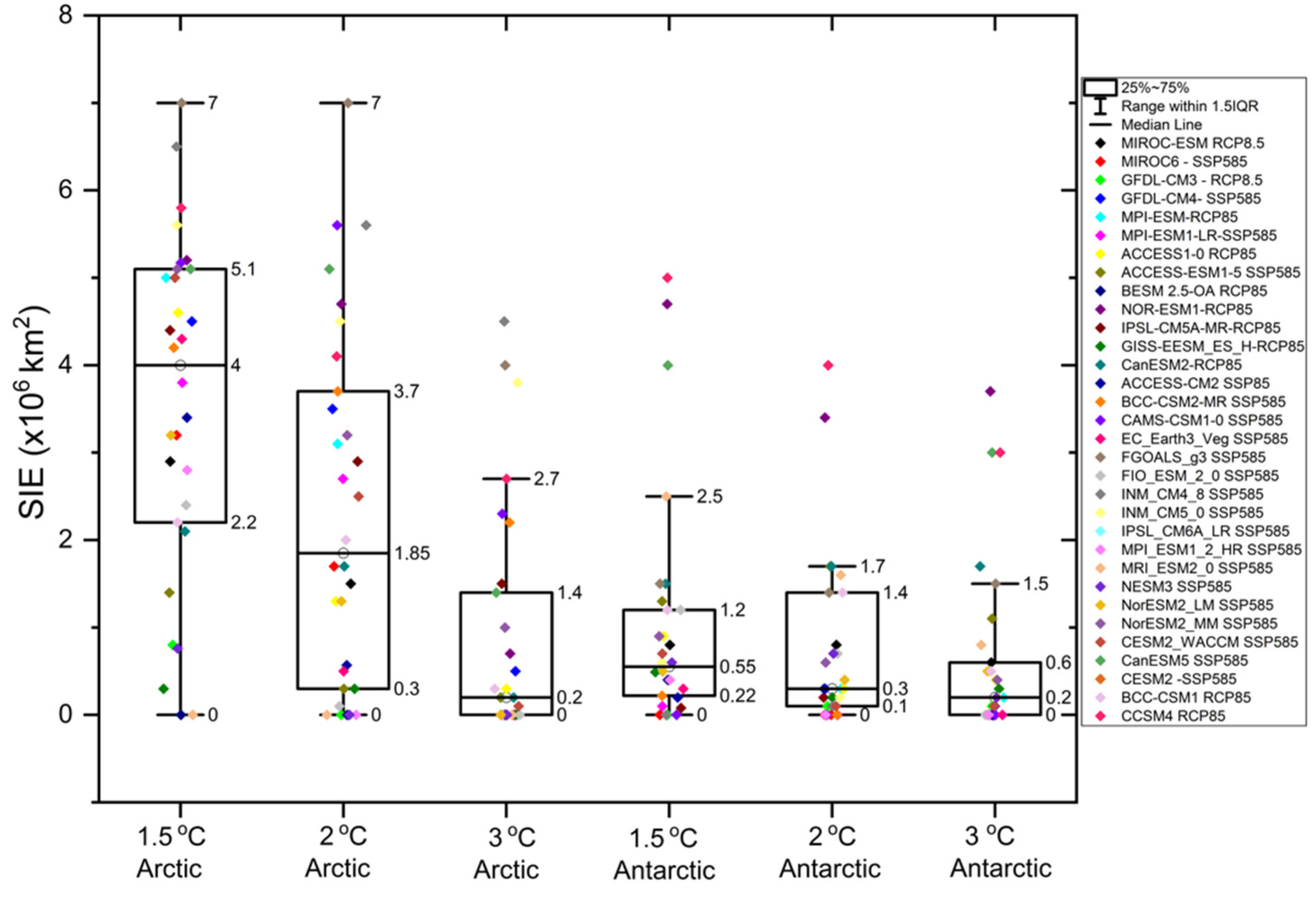
3.5. Projections of Future Ice-Free Conditions

Ice-free conditions are commonly defined as when the Arctic or Antarctica (the Southern Ocean) first becomes ice-free at the end of summer. Specifically, the first year when the average SIE in September (for the Arctic) or February (for Antarctica) falls below 1 million km². This concept has been widely used to evaluate the northern hemisphere polar regions’ sensibility to climate change. It is considered appropriate because it is expected that the north coasts of Greenland and Canada will remain with some sea ice for many years, even though the bulk of the Arctic Ocean will become ice-free, open water [5,37,45].

In this session, we investigate the SIE variability and the ice-free occurrence for each CMIP model, using RCP85 and SSP585, considering the interval time (years) between each level of warming +1.5 °C, 2.0 °C and 3.0 °C, as described in Figure 3. Therefore, we point out the number of years that each CMIP model takes to reach the warming threshold and the simulated SIE in this year and account for the numbers of the ice-free occurrence during this time interval (Figure 6 and Figure 7). In the last case and for simplification, we only analyzed the month of sea-ice minimum occurrence, that is, September for the Arctic and February for Antarctica.

Figure 6 shows the sea-ice minimum retrieved for each level of global warming in the Arctic and Antarctica. The boxes indicate the central 50% intermodal range (25–75%), the median, and upper and lower boundaries in each of the CMIP models used here. When the global warming crossed the +1.5 °C, in the time frame around the year of 2024 (Figure 3), the warming in the Arctic and Antarctica was more than twice the global warming (Figure 4 and Figure 5), and the simulated SIE minimum (Figure 6) was close to 4 × 10⁶ km² (0.55 × 10⁶ km²) for the Arctic (Antarctica). The simulated Arctic (Antarctic) sea ice interquartile ranged from 2.2 to 5.1 × 10⁶ km² (0.22 to 1.5⁵ × 10⁶ km²). The number of the years in Figure 7 indicates how many years each model takes to reach the global warming target. For instance, in Figure 7a, the CAMS-CSM1-0 model (SSP585) reached the +1.5 °C threshold after 38 years (year 2053, as shown in Figure 3). The absence of values for the Arctic ice-free occurrence (orange color bar) indicates that in this period, ice-free conditions did not occur. The opposite condition was found in simulations for Antarctica (yellow color bar): there, we have ice-free conditions in all years (since 2015) until 2053. In all February months of each year, Antarctica’s simulated SIE drops below 1 × 10⁶ km², considered the higher limit for ice-free conditions. The absence of values inside the black color bars (years) means that the respective model already reached this warming threshold at the first year of model run. For example, the models MPI-ESM (RCP85) CanESM5 (SSP585) reached the +1.5 °C threshold in 2015 (Figure 3).

For the high latitudes of the northern hemisphere, most of the models did not indicate ice-free conditions until 2024, despite the decreasing SIE values (Figure 6) compared to observed SIE (Figure 2). Only two models showed the largest occurrence of ice-free conditions in this period: BESM-OA V2.5 and MRI-ESM2-0, with respectively 17 and 14 occurrences. For high latitudes of the southern hemisphere, on the other hand, we found that SIE falls below the 1 × 10⁶ km² limit since the +1.5 °C global warming occurrence date and even before (Figure 7a,b). Therefore, for both RCP85 and SSP585 scenarios, we expect ice-free conditions in Antarctica for all Paris Agreement warming thresholds in February of every year after the global warming threshold of +1.5 °C is reached (Figure 6 and Figure 7).

Most CMIP models show an accelerating decline in the SIE summer minimum (Figure 6). The Arctic SIE minima for the +2.0 °C and 3.0 °C decrease drastically from the 4 × 10⁶ km² simulated for the +1.5 °C target to 1.85 and 0.2 × 10⁶ km², simulated in the +2.0 °C and 3.0 °C thresholds, respectively, when the Arctic Ocean becomes ice-free (Figure 6). The number of years between the +1.5 °C, 2.0 °C and 3.0 °C global warming thresholds and the respective occurrence of ice-free conditions is shown in Figure 7b–d. The ice-free occurrence gradually increased towards the warming of +3.0 °C (Figure 7c). After +2.0 °C, ice-free conditions became more frequent and evident, year after year. According to [45], ice-free conditions occur as function of the global mean temperature variability across the entire CMIP6 multi-model ensemble.

Results described in Figure 6 and Figure 7, considering RCP8.5 and SSP585, clearly suggest that both the Arctic and Antarctica will become ice-free in the forthcoming summers as a direct response to the increased atmospheric CO₂ concentrations. This is considered one of the most visible and dramatic signs of recent climate change with unknown effects not only local regions, but also far beyond the polar regions. We suggest that significant changes in the seasonal cycle of sea ice will occur. We will probably experience an earlier ending of the sea ice melting period in association with a large decrease in sea ice thickness. As a consequence, we will have a delay in the sea ice formation process. According to [37], the heat absorbed during the boreal summer as a result of sea ice shrinkage will be released during the boreal autumn, contributing to an increase in air temperatures. In this scenario, the Arctic Ocean will become covered only by “first year” sea ice, that is, the sea ice that does not survive the next summer melting season. This “first year” sea ice is thin and more vulnerable to melting, making the Arctic region even more sensitive, both dynamically and thermodynamically, to air temperature changes. We then expect to have a strong increase in leads and polynyas that promotes a very efficient heat energy exchange between the relatively warm ocean and cold atmosphere. It is worth mentioning that all our results are prone to uncertainty. The more frequent causes of the uncertainties related to the initial timing of ice-free summers for both the Arctic and Antarctica, very difficult to be directly measured and compared among the CMIP outputs, are largely related to the different physical parameterizations of each model and the natural variability [33,37,45].

4. Conclusions

State-of-the-art global climate models point out the fact that mean global air temperature is increasing and will increase further in the future, with enhanced consequences in the high latitudes of both hemispheres [7,10,13,17]. In the present paper, we investigate the effects of different warming levels, considering the Paris Agreement targets, in polar amplification and sea ice extent for both the Arctic and Antarctic regions. We showed that CMIP models are able to correctly capture the seasonal SIE cycle. However, we found a large spread in this variable among all CMIP models. We showed that this occurs all months but is relatively larger during the cold season. According to Figure 2, the Arctic SIE is better represented than the Antarctic SIE in both CMIP5 and CMIP6 simulations. The high sensitivity of the polar regions to the global atmospheric CO₂ concentration levels is described here. We showed that the Arctic region is warming faster than Antarctica and at levels at least twice as large as the global average (Figure 4 and Figure 5). Despite a smaller warming in Antarctica when compared with the Arctic (Figure 2), the warming in this region should not be neglected due to profound implications for the environment and its potential impact in modifying the ocean and the atmospheric circulations [21,23,24,27].

We found, in both CMIP5 and CMIP6 projections, that global warming crosses the +1.5 °C (+2.0 °C) around 2024 (2040). The threshold of +3.0 °C global warming is projected for the year 2063. For all targets, the global warming median values (representing the initial timing of global warming occurrence) are similar in CMIP5 and CMIP6 outputs. However, we suggest that the effects of the warming are expected to vary widely in different regions and also vary greatly in each model. We showed, clearly, that the warming signal is not symmetric, with higher values always found in the high latitudes of the northern hemisphere. The simulated warming in the Arctic was found to be close to 3.6 °C and 4.5 °C) for the respective +1.5 °C and +2.0 °C Paris Agreement targets. Considering the +3.0 °C global warming threshold, the simulated median warming was close to 6.6 °C. The equivalent warmings simulated for all Paris Agreement targets were similar, with values above twice as larger as the global mean (2.4, 2.3 and 2.2 times for the +1.5 °C, 2.0 °C and 3.0 °C global warming thresholds, respectively).

For Antarctica, the median warmings simulated for the +1.5 °C and 2.0 °C global warming thresholds were 1.5 °C and 2.1 °C, respectively (Figure 4). When global warming crosses the +1.5 °C threshold around the year 2024, the local warming was more than twice as large as the global warming (Figure 1, Figure 2, Figure 3, Figure 4 and Figure 5). In this situation, the simulated SIE minimum in Antarctica was close to 0.55 × 10⁶ km². In this time frame, the SIE minimum in the Arctic was 4 × 10⁶ km². For northern hemisphere high latitudes, most models did not indicate ice-free conditions until 2024 (Figure 6). On the other hand, around Antarctica, the SIE falls below the minimum limit of 1 × 10⁶ km² since the +1.5 °C global warming threshold was achieved and even before that. Consequently, for both RCP85 and SSP585 scenarios, we expect summer ice-free conditions in Antarctica for all global warming thresholds.

We showed that most CMIP models show an accelerating decline in the summer minimum SIE. The Arctic SIE minimum for the +2.0 °C and 3.0 °C global warming thresholds drastically decreases with respect to the 4 × 10⁶ km² simulated in +1.5 °C target to 1.85 × 10⁶ km² and 0.2 × 10⁶ km² simulated in the 2.0 °C and 3.0 °C thresholds, respectively, when the Arctic Ocean becomes ice-free. The ice-free occurrence gradually increases towards the warming of +3.0 °C. After the +2.0 °C threshold, the ice-free conditions become more frequent and evident throughout the years. Results presented in Figure 6 and Figure 7 clearly suggest that both the Arctic and Antarctica will become ice-free in summer in response to the imposed atmospheric CO₂ forcing.

The coupled ocean-atmosphere-sea ice physical processes sensible to the atmospheric CO₂ forcing in high latitudes are complex and act in multiple temporal and spatial scales [12,13,15,16,20]. This is considered a hot topic in the current scientific literature, for it represents one of the most visible signs of climate change in the planet, with yet unknown effects extending far behind the polar regions [10,11,13]. In the near future, more studies are needed to better understand these processes, especially including the physics of the ice sheet, a process still very poorly explored in CMIP simulations.

References

1. UNFCCC. The Paris Agreement. Available online: https://unfccc.int/process-and-meetings/the-paris-agreement/the-paris-agreement (accessed on 31 August 2021).
2. Farinosi, F.; Dosio, A.; Calliari, E.; Seliger, R.; Alfieri, L.; Naumann, G. Will the Paris Agreement protect us from hydro-meteorological extremes? Environ. Res. Lett. 2020, 15, 104037. [Google Scholar] [CrossRef]
3. Jacob, D.; Kotova, L.; Teichmann, C.; Sobolowski, S.P.; Vautard, R.; Donnelly, C.; Koutroulis, A.; Grillakis, M.; Tsanis, I.K.; Damm, A.; et al. Climate Impacts in Europe Under +1.5 °C Global Warming. Earth’s Future 2018, 6, 264–285. [Google Scholar] [CrossRef] [Green Version]
4. Lewis, S.C.; King, A.D.; Perkins-Kirkpatrick, S.; Mitchell, D. Regional hotspots of temperature extremes under 1.5 °C and 2 °C of global mean warming. Weather. Clim. Extremes 2019, 26, 100233. [Google Scholar] [CrossRef]
5. Screen, J.A.; Williamson, D. Ice-Free Arctic at 1.5 °C? Nat. Clim. Chang. 2017, 7, 230–231. [Google Scholar] [CrossRef] [Green Version]
6. King, A.D.; Harrington, L.J. The Inequality of Climate Change From 1.5 to 2 °C of Global Warming. Geophys. Res. Lett. 2018, 45, 5030–5033. [Google Scholar] [CrossRef]
7. IPCC. Climate Change 2014: Synthesis Report; Intergovernmental Panel on Climate Change (IPCC): Geneva, Switzerland, 2014; ISBN 9789291691432. [Google Scholar]
8. Sigmond, M.; Fyfe, J.C.; Swart, N.C. Ice-free Arctic projections under the Paris Agreement. Nat. Clim. Chang. 2018, 8, 404–408. [Google Scholar] [CrossRef]
9. Mitchell, D.; James, R.; Forster, P.M.; Betts, R.A.; Shiogama, H.; Allen, M. Realizing the impacts of a 1.5 °C warmer world. Nat. Clim. Chang. 2016, 6, 735–737. [Google Scholar] [CrossRef] [Green Version]
10. Smith, D.M.; Screen, J.A.; Deser, C.; Cohen, J.; Fyfe, J.C.; García-Serrano, J.; Jung, T.; Kattsov, V.; Matei, D.; Msadek, R.; et al. The Polar Amplification Model Intercomparison Project (PAMIP) contribution to CMIP6: Investigating the causes and consequences of polar amplification. Geosci. Model Dev. 2019, 12, 1139–1164. [Google Scholar] [CrossRef] [Green Version]
11. Serreze, M.C.; Barry, R. Processes and impacts of Arctic amplification: A research synthesis. Glob. Planet. Chang. 2011, 77, 85–96. [Google Scholar] [CrossRef]
12. Stuecker, M.F.; Bitz, C.M.; Armour, K.C.; Proistosescu, C.; Kang, S.M.; Xie, S.-P.; Kim, D.; McGregor, S.; Zhang, W.; Zhao, S.; et al. Polar amplification dominated by local forcing and feedbacks. Nat. Clim. Chang. 2018, 8, 1076–1081. [Google Scholar] [CrossRef]
13. Salzmann, M. The polar amplification asymmetry: Role of Antarctic surface height. Earth Syst. Dyn. 2017, 8, 323–336. [Google Scholar] [CrossRef] [Green Version]
14. Graversen, R.G.; Langen, P.L. On the Role of the Atmospheric Energy Transport in 2 × CO2–Induced Polar Amplification in CESM1. J. Clim. 2019, 32, 3941–3956. [Google Scholar] [CrossRef]
15. Pithan, F.; Mauritsen, T. Arctic amplification dominated by temperature feedbacks in contemporary climate models. Nat. Geosci. 2014, 7, 181–184. [Google Scholar] [CrossRef]
16. Screen, J.A.; Deser, C.; Simmonds, I. Local and remote controls on observed Arctic warming. Geophys. Res. Lett. 2012, 39. [Google Scholar] [CrossRef] [Green Version]
17. Serreze, M.C.; Francis, J.A. The Arctic Amplification Debate. Clim. Chang. 2006, 76, 241–264. [Google Scholar] [CrossRef] [Green Version]
18. Bekryaev, R.V.; Polyakov, I.V.; Alexeev, V. Role of Polar Amplification in Long-Term Surface Air Temperature Variations and Modern Arctic Warming. J. Clim. 2010, 23, 3888–3906. [Google Scholar] [CrossRef]
19. Hall, A. The Role of Surface Albedo Feedback in Climate. J. Clim. 2003, 17, 1550–1568. [Google Scholar] [CrossRef] [Green Version]
20. Vihma, T. Effects of Arctic Sea Ice Decline on Weather and Climate: A Review. Surv. Geophys. 2014, 35, 1175–1214. [Google Scholar] [CrossRef] [Green Version]
21. Parkinson, C.L. A 40-y record reveals gradual Antarctic sea ice increases followed by decreases at rates far exceeding the rates seen in the Arctic. Proc. Natl. Acad. Sci. USA 2019, 116, 14414–14423. [Google Scholar] [CrossRef] [Green Version]
22. Holland, P.R. The seasonality of Antarctic sea ice trends. Geophys. Res. Lett. 2014, 41, 4230–4237. [Google Scholar] [CrossRef] [Green Version]
23. Turner, J.; Phillips, T.; Marshall, G.J.; Hosking, J.S.; Pope, J.O.; Bracegirdle, T.J.; Deb, P. Unprecedented springtime retreat of Antarctic sea ice in 2016. Geophys. Res. Lett. 2017, 44, 6868–6875. [Google Scholar] [CrossRef] [Green Version]
24. Bintanja, R.; van Oldenborgh, G.; Katsman, C. The effect of increased fresh water from Antarctic ice shelves on future trends in Antarctic sea ice. Ann. Glaciol. 2015, 56, 120–126. [Google Scholar] [CrossRef] [Green Version]
25. Marshall, J.C.; Armour, K.C.; Scott, J.R.; Kostov, Y.K.; Hausmann, U.; Ferreira, D.; Shepherd, T.G.; Bitz, C. The ocean’s role in polar climate change: Asymmetric Arctic and Antarctic responses to greenhouse gas and ozone forcing. Philos. Trans. R. Soc. A Math. Phys. Eng. Sci. 2014, 372, 20130040. [Google Scholar] [CrossRef] [PubMed] [Green Version]
26. Swart, N.C.; Fyfe, J.C. The influence of recent Antarctic ice sheet retreat on simulated sea ice area trends. Geophys. Res. Lett. 2013, 40, 4328–4332. [Google Scholar] [CrossRef]
27. Bintanja, R.; Van Oldenborgh, G.J.; Drijfhout, S.S.; Wouters, B.; Katsman, C.A. Important role for ocean warming and increased ice-shelf melt in Antarctic sea-ice expansion. Nat. Geosci. 2013, 6, 376–379. [Google Scholar] [CrossRef]
28. Shu, Q.; Wang, Q.; Song, Z.; Qiao, F.; Zhao, J.; Chu, M.; Li, X. Assessment of Sea Ice Extent in CMIP6 With Comparison to Observations and CMIP5. Geophys. Res. Lett. 2020, 47, e2020GL087965. [Google Scholar] [CrossRef]
29. Roach, L.A.; Dörr, J.; Holmes, C.R.; Massonnet, F.; Blockley, E.W.; Notz, D.; Rackow, T.; Raphael, M.N.; O’farrell, S.; Bai-ley, D.A.; et al. Antarctic Sea Ice Area in CMIP6. Geophys. Res. Lett. 2020, 47. [Google Scholar] [CrossRef]
30. Shu, Q.; Song, Z.; Qiao, F. Assessment of sea ice simulations in the CMIP5 models. Cryosphere 2015, 9, 399–409. [Google Scholar] [CrossRef] [Green Version]
31. Turner, J.; Bracegirdle, T.; Phillips, T.; Marshall, G.J.; Hosking, S. An Initial Assessment of Antarctic Sea Ice Extent in the CMIP5 Models. J. Clim. 2013, 26, 1473–1484. [Google Scholar] [CrossRef]
32. Stroeve, J.C.; Kattsov, V.; Barrett, A.; Serreze, M.; Pavlova, T.; Holland, M.; Meier, W. Trends in Arctic sea ice extent from CMIP5, CMIP3 and observations. Geophys. Res. Lett. 2012, 39. [Google Scholar] [CrossRef] [Green Version]
33. Casagrande, F.; de Souza, R.B.; Nobre, P.; Marquez, A.L. An inter-hemispheric seasonal comparison of polar amplification using radiative forcing of a quadrupling CO2 experiment. Ann. Geophys. 2020, 38, 1123–1138. [Google Scholar] [CrossRef]
34. Diebold, F.X.; Rudebusch, G.D.; Barrett, A.; Goulet Coulombe, P.; Engle, R.; Göbel, M.; Hankel, C.; Hausfather, Z.; Hen-Dry, D.; Hillebrand, E.; et al. Nber Working Paper Series Probability Assessments of an Ice-Free Arctic: Comparing Statistical and Climate Model Projections. J. Econom. 2021. Available online: https://www.nber.org/papers/w28228 (accessed on 5 September 2021). [CrossRef]
35. Cohen, J.; Screen, J.A.; Furtado, J.; Barlow, M.; Whittleston, D.; Coumou, D.; Francis, J.A.; Dethloff, K.; Entekhabi, D.; Overland, J.E.; et al. Recent Arctic amplification and extreme mid-latitude weather. Nat. Geosci. 2014, 7, 627–637. [Google Scholar] [CrossRef] [Green Version]
36. Tang, Q.; Zhang, X.; Yang, X.; Francis, J.A. Cold winter extremes in northern continents linked to Arctic sea ice loss. Environ. Res. Lett. 2013, 8, 014036. [Google Scholar] [CrossRef]
37. Wang, M.; Overland, J.E. A sea ice free summer Arctic within 30 years? Geophys. Res. Lett. 2009, 36. [Google Scholar] [CrossRef] [Green Version]
38. Schleussner, C.-F.; Rogelj, J.; Schaeffer, M.; Lissner, T.; Licker, R.; Fischer, E.M.; Knutti, R.; Levermann, A.; Frieler, K.; Hare, W. Science and policy characteristics of the Paris Agreement temperature goal. Nat. Clim. Chang. 2016, 6, 827–835. [Google Scholar] [CrossRef] [Green Version]
39. Taylor, K.E.; Stouffer, R.J.; Meehl, G.A. An Overview of CMIP5 and the Experiment Design. Bull. Am. Meteorol. Soc. 2012, 93, 485–498. [Google Scholar] [CrossRef] [Green Version]
40. O’Neill, B.C.; Tebaldi, C.; van Vuuren, D.P.; Eyring, V.; Friedlingstein, P.; Hurtt, G.; Knutti, R.; Kriegler, E.; Lamarque, J.-F.; Lowe, J.; et al. The Scenario Model Intercomparison Project (ScenarioMIP) for CMIP6. Geosci. Model Dev. 2016, 9, 3461–3482. [Google Scholar] [CrossRef] [Green Version]
41. Eyring, V.; Bony, S.; Meehl, G.A.; Senior, C.A.; Stevens, B.; Stouffer, R.J.; Taylor, K.E. Overview of the Coupled Model Intercomparison Project Phase 6 (CMIP6) experimental design and organization. Geosci. Model Dev. 2016, 9, 1937–1958. [Google Scholar] [CrossRef] [Green Version]
42. Cavalieri, D.J.; Parkinson, C.L.; Gloersen, P.; Zwally, H.J. Sea Ice Concentrations from Nimbus-7 SMMR and DMSP SSM/I-SSMIS Passive Mi-Crowave Data; Version 1; 1996; Available online: https://doi.org/10.5067/8GQ8LZQVL0VL (accessed on 5 September 2021).
43. Sorteberg, A.; Kattsov, V.; Walsh, J.; Pavlova, T. The Arctic surface energy budget as simulated with the IPCC AR4 AOGCMs. Clim. Dyn. 2007, 29, 131–156. [Google Scholar] [CrossRef]
44. Karlsson, J.; Svensson, G. Consequences of poor representation of Arctic sea-ice albedo and cloud-radiation interactions in the CMIP5 model ensemble. Geophys. Res. Lett. 2013, 40, 4374–4379. [Google Scholar] [CrossRef]
45. Notz, D. SIMIP Community Arctic Sea Ice in CMIP6. Geophys. Res. Lett. 2020, 47, e2019GL086749. [Google Scholar] [CrossRef]
46. Skagseth, Ø.; Furevik, T.; Ingvaldsen, R.; Loeng, H.; Mork, A.; Orvik, A.; Ozhigin, V. Volume and Heat Transports to the Arctic Ocean via the Norwegian and Barents Seas; Springer: Dordrecht, The Netherland, 2008. [Google Scholar]
47. Previdi, M.; Janoski, T.P.; Chiodo, G.; Smith, K.L.; Polvani, L.M. Arctic Amplification: A Rapid Response to Radiative Forcing. Geophys. Res. Lett. 2020, 47, e2020GL089933. [Google Scholar] [CrossRef]
48. Stjern, C.W.; Lund, M.T.; Samset, B.H.; Myhre, G.; Forster, P.M.; Andrews, T.; Boucher, O.; Faluvegi, G.; Fläschner, D.; Iversen, T.; et al. Arctic Amplification Response to Individual Climate Drivers. J. Geophys. Res. Atmos. 2019, 124, 6698–6717. [Google Scholar] [CrossRef]
49. Singh, H.A.; Rasch, P.J.; Rose, B.E.J. Increased Ocean Heat Convergence Into the High Latitudes With CO2 Doubling Enhances Polar-Amplified Warming. Geophys. Res. Lett. 2017, 44, 10583–10591. [Google Scholar] [CrossRef]
50. Zhang, X.; Li, X.; Chen, D.; Cui, H.; Ge, Q. Overestimated climate warming and climate variability due to spatially homogeneous CO2 in climate modeling over the Northern Hemisphere since the mid-19th century. Sci. Rep. 2019, 9, 17426. [Google Scholar] [CrossRef]
51. Navarro, A.; Moreno, R.; Tapiador, F.J. Improving the representation of anthropogenic CO2 emissions in climate models: Impact of a new parameterization for the Community Earth System Model (CESM). Earth Syst. Dyn. 2018, 9, 1045–1062. [Google Scholar] [CrossRef] [Green Version]
52. Overland, J.E.; Wang, M. The 2020 Siberian heat wave. Int. J. Clim. 2020, 41, E2341–E2346. [Google Scholar] [CrossRef]
53. Hanna, E.; Nolan, J.E.; Overland, J.E.; Hall, R.J. Climate Change in the Arctic. Arct. Ecol. 2021, 168, 9. [Google Scholar] [CrossRef]
54. Bromwich, D.H.; Nicolas, J.P.; Monaghan, A.; Lazzara, M.; Keller, L.M.; Weidner, G.A.; Wilson, A.B. Central West Antarctica among the most rapidly warming regions on Earth. Nat. Geosci. 2012, 6, 139–145. [Google Scholar] [CrossRef] [Green Version]
55. Turner, J.; Dennis, P.; Vaughan, D.G.; Marshall, G.J.; Connolley, W.M.; Parkinson, C.; Mulvaney, R.; Hodgson, D.A.; King, J.C.; Pudsey, C.J. Recent Rapid Regional Climate Warming on the Antarctic Peninsula Related Papers Ice Core Evidence for Significant 100-Year Regional Warming on t He Ant Arct Ic Peninsula Recent Rapid Regional Cli-Mate Warming on the Antarctic Peninsula. Clim. Chang. 2003. Available online: https://link.springer.com/article/10.1023/A:1026021217991#citeas (accessed on 5 September 2021).
56. Pfeifer, S.; Rechid, D.; Reuter, M.; Viktor, E.; Jacob, D. 1.5°, 2°, and 3° Global Warming: Visualizing European Regions 722 Affected by Multiple Changes. Reg. Environ. Chang. 2019, 19, 1777–1786. [Google Scholar] [CrossRef] [Green Version]
57. Tobin, I.; Greuell, W.; Jerez, S.; Ludwig, F.; Vautard, R.; van Vliet, M.T.; Bréon, F.-M. Vulnerabilities and resilience of European power generation to 1.5 °C, 2 °C and 3 °C warming. Environ. Res. Lett. 2018, 13, 044024. [Google Scholar] [CrossRef]
58. Donnelly, C.; Greuell, W.; Andersson, J.; Gerten, D.; Pisacane, G.; Roudier, P.; Ludwig, F. Impacts of climate change on European hydrology at 1.5, 2 and 3 degrees mean global warming above preindustrial level. Clim. Chang. 2017, 143, 13–26. [Google Scholar] [CrossRef] [Green Version]
59. Kjellström, E.; Nikulin, G.; Strandberg, G.; Christensen, O.B.; Jacob, D.; Keuler, K.; Lenderink, G.; van Meijgaard, E.; Schär, C.; Somot, S.; et al. European climate change at global mean temperature increases of 1.5 and 2 °C above pre-industrial conditions as simulated by the EURO-CORDEX regional climate models. Earth Syst. Dyn. 2018, 9, 459–478. [Google Scholar] [CrossRef] [Green Version]
60. Vautard, R.; Gobiet, A.; Sobolowski, S.; Kjellström, E.; Stegehuis, A.I.; Watkiss, P.; Mendlik, T.; Landgren, O.; Nikulin, G.; Teichmann, C.; et al. The European climate under a 2 °C global warming. Environ. Res. Lett. 2014, 9, 034006. [Google Scholar] [CrossRef]
61. Hahn, L.C.; Armour, K.C.; Zelinka, M.D.; Bitz, C.M.; Donohoe, A. Contributions to Polar Amplification in CMIP5 and CMIP6 Models. Front. Earth Sci. 2021, 9. [Google Scholar] [CrossRef]
62. Hahn, L.C.; Armour, K.C.; Battisti, D.S.; Donohoe, A.; Pauling, A.G.; Bitz, C.M. Antarctic Elevation Drives Hemispheric Asymmetry in Polar Lapse Rate Climatology and Feedback. Geophys. Res. Lett. 2020, 47, e2020GL088965. [Google Scholar] [CrossRef]
Figure 1. (a) Arctic and (b) Antarctic SIE seasonal cycle as simulated by CMIP5 (light gray rectangle) and CMIP6 (dark gray rectangle), respectively related to the period 1980–2005 and 1980–2014. Satellite observations for the respective months are represented by the black lines. The boxplots indicate the central 50% intermodal range (25–75%), the median and the upper and lower limit in CMIP5 and CMIP6 under historical experiment. The green triangle shows the average value of the set of models. The black diamond represents the outline values.
Atmosphere 12 01494 g001
Figure 2. (a) Global map of the polar amplification measure obtained from long-term observations of the near-surface air temperature (°C) for the 2010–2020 period relative to the 1980–1990 period. (b) Zonal mean of the near-surface temperature (°C) for the 2010–2020 period relative to the 1980–1990 period.
Atmosphere 12 01494 g002
Figure 3. The central year at which CMIP models reach the temperature threshold of +1.5 °C, 2.0 °C and 3.0 °C global mean warming. The boxplots indicate the central 50% intermodal range (25–75%), the median and the upper and lower boundaries in CMIP5 and CMIP6 under RCP8.5 and SSP585 scenarios.
Atmosphere 12 01494 g003
Figure 4. Polar Amplification simulated by CMIP5 and CMIP6 climate models for the temperature thresholds of +1.5 °C, 2.0 °C and 3.0 °C global mean warming under RCP8.5 and SSP585 scenarios of northern and southern hemispheres high latitudes. The boxplot was defined by using two lines at the 25th percentile and 75th percentile. The 25th percentile is the value at which 25% of the data values are below this value. Thus, the middle 50% of the data values fall between the 25th percentile and the 75th percentile. The distance between the upper (75th percentile) and lower (25th percentile) lines of the box is the inter-quartile range.
Atmosphere 12 01494 g004
Figure 5. Warming rate of the Polar Amplification simulated by CMIP5 and CMIP6 climate models for the temperature thresholds of +1.5 °C, 2.0 °C and 3.0 °C global mean warming under RCP8.5 and SSP585 scenarios of northern (HN) and southern (SH) hemispheres high latitudes. The boxplot indicates the central 50% intermodal range (25–75%), the median and upper and lower boundaries in the CMIP models.
Atmosphere 12 01494 g005
Figure 6. Arctic and Antarctic SIE summer minimum considering the temperature threshold of +1.5 °C, 2.0 °C and 3.0 °C global mean warming under RCP8.5 and SSP585 scenarios. The Arctic’s (Antarctica’s) summer minimum occurs in September (March).
Atmosphere 12 01494 g006
Figure 7. Number of years that each model takes to reach the different global warming thresholds (black bars). The number of summer ice-free occurrences in the Arctic (Antarctica) for each CMIP model are represented by the orange (yellow) bars. (a) Up to +1.5 °C threshold; (b) the period between the +1.5 °C and +2 °C global warming thresholds; (c) the period between the +2 °C and +3 °C global warming thresholds; and (d) the period between the +3 °C global warming thresholds and onwards until 2100 (end of simulation).
Atmosphere 12 01494 g007
Publisher’s Note: MDPI stays neutral with regard to jurisdictional claims in published maps and institutional affiliations.