Abstract
In recent years, evidence of recent climate change has been identified in South America, affecting agricultural production negatively. In response to this, our study employs a crop modelling approach to estimate the effects of recent climate change on maize yield in four provinces of Ecuador. One of them belongs to a semi-arid area. The trend analysis of maximum temperature, minimum temperature, precipitation, wind speed, and solar radiation was done for 36 years (from 1984 to 2019) using the Mann–Kendall test. Furthermore, we simulated (using the LINTUL5 model) the counterfactual maize yield under current crop management in the same time-span. During the crop growing period, results show an increasing trend in the temperature in all the four studied provinces. Los Rios and Manabi showed a decreasing trend in radiation, whereas the semi-arid Loja depicted a decreasing precipitation trend. Regarding the effects of climate change on maize yield, the semi-arid province Loja showed a more significant negative impact, followed by Manabi. The yield losses were roughly 40 kg ha and 10 kg ha per year, respectively, when 250 kg N ha is applied. The simulation results showed no effect in Guayas and Los Rios. The length of the crop growing period was significantly different in the period before and after 2002 in all provinces. In conclusion, the recent climate change impact on maize yield differs spatially and is more significant in the semi-arid regions.
1. Introduction
Agriculture is an important sector of the Ecuadorian economy with a gross domestic product (GDP) share of 9.2% [1]. The sector specially offers several employment opportunities in the rural area, boosting food security and promoting exports. Maize occupies the fourth place by production area among all crops in Ecuador and is the second most-consumed item by the population after rice [2].
According to the fifth report of the Intergovernmental Panel on Climate Change (IPCC), the last three decades have been the warmest period of the last 1400 years, particularly in the North Hemisphere. The mean global temperature increased by 0.65 to 1.06 °C in the period from 1880 to 2012 [3]. Particularly, an increasing trend in temperature has been observed in South America since roughly 1975. The increment in the last four decades has been about 0.7–1 °C. Whereas, the precipitation has shown a spatial variability, increasing in some parts of southeastern South America and decreasing in other places around Central America. Furthermore, anomalies such as droughts and floods have been identified more frequently [3]. In Ecuador, authors have reported a warming trend in temperature from the mid-1940s to the mid-2000s, based on the observations of meteorological stations of the Ecuadorian Institute of Meteorology and Hydrology [4,5,6]. Moreover, semi-arid regions located in the southern part of Ecuador, where agriculture remains to be the main economic activity, characterized by low rainwater availability, are more prone to climate change effects [7,8,9].
The impact of recent climate change on specific crops in Ecuador has been marginally investigated. However, a study demonstrated that some maize farmers moved their cultivation areas to higher altitudes due to the temperature increase in low-altitude areas [10]. Another work reported that banana yield losses are correlated with decreasing rainfall. The temperature increment could potentially contribute to the expansion of production areas [11]. There is no work studying the effects of recent climate change on the maize yield in the most important production regions in Ecuador, including semi-arid areas, to the best of our knowledge.
However, it is not possible to assess the impact of climate change on the historical maize yield in Ecuador by analyzing the statistical yields of the Ecuadorian Ministry of Agriculture because the yield changes in the last 50 years are affected by both climate change and increasing N application rates. According to the Ecuadorian Ministry of Agriculture’s annual statistical report, the maize yield in Ecuador has risen by more than 100% in the last decade. A significant part of this improvement could be attributed to the subsidized certified seeds, fertilizers, and pesticides by the local government [12]. Nonetheless, the increase in the maize yield shown by these Ecuadorian institutions is not consistent with the observed impact of recent climatic change at the global scale, where the maize yield decline was estimated to 3.8% compared with its counterfactual scenario of no climate change [13]. For that reason, in this study, we investigate whether the recent climate change has affected maize yields and its growing period length in four provinces of Ecuador, and we try to quantify the climate change impact. A crop model approach was required to build the counterfactual yield.
2. Materials and Methods
2.1. Study Area and Simulation Units
This crop model-based study was conducted across four administrative zones (called provinces) of Ecuador, a South-American country located between the Pacific Ocean and the Amazon rainforest. The geographical locations subject to the study are depicted in Figure 1. Due to its tropical location, Ecuador is characterized by two seasons: the wet season or winter, and the dry season or summer.
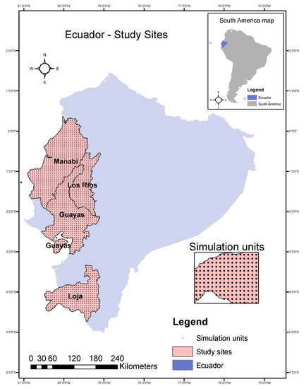
Figure 1.
Four provinces of Ecuador where maize yield was simulated: Guayas, Los Rios, Loja, and Manabi. Each dot represents a simulation unit, in grid cells at 0.05° × 0.05°.
Furthermore, the duration of each season varies regionally. For instance, in the coastal region, the wet season lasts from December to May, and the dry season from June until November. Besides the corresponding climate patterns, in this study, we analyzed the effects of recent climate change on maize yield for the provinces of Guayas, Manabi, Los Rios, and the semi-arid province Loja.
Guayas is an administrative zone of 15,430 km [14] located on the coast of Ecuador between the longitudes 79°05′ W and 80°33′ W and latitudes between 0°50′ S and 3°04′ S. The altitude varies between 0 and 100 MASL, which comprises mainly a flat relief. The average temperature lies between 24 °C to 27 °C. The mean monthly precipitation in the rainy season is between 100 and 500 mm, and during the dry season is between 4 and 30 mm [15]. Guayas has alluvial and fluvial-marine plains with a diverse range of soils derived from alluvial sands, silts, and clays [16].
Manabi is also located on the Ecuadorian coast and lies between longitudes 79°26′ W and 80°56′ W, and latitudes between 0°22′ S and 1°56′ S. It has a surface area of 18,940 km and is bordered to the north by Esmeraldas, south by Santa Elena, east by Los Rios and Guayas, and west by the Pacific Ocean. Its altitude lies between 0 and 500 MASL, and the average daily temperature varies from 24 °C to 26 °C. The mean monthly rainfall in the wet season lies between 80 and 190 mm, and during the dry season is from 9 mm to 60 mm [17]. Geographically, Manabi has hills, plateaus, and gentle slope hills with vertic soils composed of silty clay to clay texture [18].
Los Rios, with a surface area of 7205 km and altitude between 0 and 500 MASL, lies between the latitudes 0°31′ S and 2°08′ S and longitudes from 79°14′ W and 79°53′ W. Its border lies directly at the foot of the Andean Mountains, which produces particular climate conditions. During the wet season, the mean monthly precipitation stays between 150 and 460 mm, and during the dry season between 12 and 54 mm. The daily average temperature ranges from 24 °C to 26.5 °C [19]. This province is highly productive for agriculture because of its fertile soils such as andisols, which have high humus content [18].
Loja is located in the south Andean region of Ecuador and borders Peru. It is characterized by its semi-arid conditions [8]. Geographically, its territory comprises highlands and lowlands. It lies between the latitudes 3°19′ S and 4°44′ S and longitudes from 79°05′ W and 80°29′ W. Its altitude ranges from 100 MASL to 2000 MASL, and the total surface area is 11,063 km [14]. The mean monthly precipitation during the wet season is between 90 and 190 mm, and during the dry season ranges from 12 to 70 mm. The daily average temperature lies between 20 °C and 21 °C [20]. Due to its topography, Loja has diverse soils such as non-colluvial black, silty andosols with high humus content, and ferralitic soils [18].
2.2. Climate and Soil Data
For this study, we used climate data from the publicly available repository Nasa Power [21]. These data are available at a spatial resolution of 0.5° latitude by 0.5° longitude. The dataset is based on a single assimilation model from Goddard’s Global Modelling and Assimilation Office (GMAO). The meteorological data comes from the GMAO Modern-Era Retrospective-Analysis for Research and Applications (MERRA-2) assimilation model products [22]. The used data in this study spans the period from 1984 to 2019 on a daily scale. The following parameters were considered: maximum and minimum air temperature at 2 m (°C), wind speed at 10 m (m s), precipitation (mm), and solar radiation on the horizontal surface (MJ m).
For soil input data, we leveraged the soil property worldwide maps of the SoilGrids database available in the ISRIC Data Hub [23], which have an original resolution of 250 × 250 m. However, we extracted the soil parameters at the resolution of our simulation units (0.05° × 0.05°). Specifically, the parameters extracted from the dataset are sand, silt, clay, organic carbon, and bulk density at six distinct depths (0.5, 0.15, 0.30, 0.60, 1.0, 2.0 m). Based on these parameters, we computed the soil water content at field capacity, wilting point and saturation point using the Van-Genuchten parameters according to Rawls et al. (1993) [24].
Finally, the model simulations were carried out for each simulation unit (refer Figure 1), which is a combination of climate data at ° resolution and the soil data at ° resolution. It implies that we ran the simulation at each ° grid point and aggregated the final simulation outputs to the province level.
2.3. Climate Change Analysis
Our work analyzes a time-series of climate parameters for each simulation unit in Ecuador (see Figure 1) for each year from 1984 to 2019. Specifically, the parameters under study are maximum temperature, minimum temperature, precipitation, wind speed, and radiation at a daily time scale. Solar radiation was assessed only from 1984 to 2007 since Nasa Power used different data sets to get a long time series of radiation (until 2019) and it is not recommended to assess trends across the breaks in the data source.
The average of each parameter was plotted and analyzed on a monthly basis, full-year basis, and during the maize crop growing period (January to May). For our study, the crop growing period is the time-span when the maize is cultivated in Ecuador that belongs to the wet season (higher precipitation) from January to May.
To assess the existence of climate change, we used the Mann–Kendall trend test (see Appendix A for more details). This statistical test is one of the most frequently used non-parametric test for non-normal distributed data. Since Ecuador is commonly affected by ENSO phenomenon, climate data is prone to contain anomalies, further referred to as outliers by the statistical test. It is another powerful reason to rely on the robustness of the Mann–Kendall test, as it allows effective treatment of outliers [25,26].
For our study, we considered a yearly temporal resolution of the time series from 1984 to 2019. The evaluated time series was the average of each climate parameter over the full-year and maize crop growing period (January to June). Regarding the spatial reference, each grid cell’s means were aggregated over each province to have a unique value per year and calculate the delta.
Furthermore, the Seasonal Mann–Kendall was applied in the monthly time series. It is a particular case of the general Mann–Kendall, which runs the test on each of n seasons separately, where n is the number of seasons. In our case, the Seasonal Mann–Kendall was set up to compare each parameter for the same month every year (e.g., January value of one year compared with the following year’s January value).
In our study, the null hypothesis (H0) indicates no trend in the historical climate records, and the alternative hypothesis (H1) is a strong indication for a positive or negative trend. The level of significance to accept or reject the H0 was . Based on the Mann–Kendall test results, all the regions with at least one significant trend in any of the climate parameters are considered a location with the presence of climate change.
To assess the trend magnitude, we computed the Sen’s slope over the analyzed parameters’ data series. It allows us to quantitatively assess the climate change expressed as the rate of variation of the corresponding slope. This value is computed for a data series as the median of the output of Equation (1).
2.4. Crop Model Description
The crop simulations were carried out through the LINTUL5 model within the SIMPLACE (Scientific Impact Assessment and Modelling Platform for Advanced Crop and Ecosystem Management). This model mimics the plant growth and calculates the biomass production depending on the photosynthetically active radiation (PAR) and the radiation use efficiency (RUE). In LINTUL5, each phenological development stage depends on the heat units (temperature sum), which is the cumulative daily effective temperature specific for each crop [27].
Additionally, LINTUL5 model simulates water and nutrient-limited crop production. Water stress is exhibited when the available soil water exceeds the field capacity or between the critical and wilting points. It is expressed via a growth reduction factor, which limits the growth and biomass production. A reduction factor can also express the limitation of nutrients, so in case of sub-optimal nitrogen availability for the crop, the model applies a stress factor that reduces the rate of biomass production [28].
The climate parameters (precipitation, minimum and maximum temperature, wind speed, radiation, concentration), applied nutrients (N, P, K), and soil properties (texture, organic carbon, bulk density, field capacity, wilting point) are the input for the model. They will also define biomass’s daily production, leaf area index development, root growth, and yield. The biomass is partitioned within various organs (leaves, stems, roots, and grains), and its allocation works as a function of a fraction dependent on the development stage.
LINTUL5 model has been widely used to assess the cropping systems, determine yield gaps and, evaluate the effects of climate change. For example, a study investigated the impact of grid-based time series of climate variables assembled from the same data source and several sources on maize yield in Ghana, Ethiopia, and Nigeria [29]. Another study evaluated heat stress responses on maize crops in Argentina, and Spain [30]. Srivastava et al. studied the effects of climate variables on potential maize productivity, and an assessment of future climate scenarios (RCP 4.5 and RCP 8.5) in central Ghana [31].
Furthermore, two components, SlimWater and SoilCN, were coupled to LINTUL5. The former enables the soil-water balance, and the latter simulates the soil organic matter dynamics and works for transferring the crop residues to the soil. We denote the resulting framework with all the components as SIMPLACE<LINTUL5-SlimWater-SoilCN>.
SlimWater applies the water balance of multiple layer soil profiles instead of the two-layer provided by default in LINTUL 5. The changes in soil waters depend on the uptake by the crop, evaporation, surface run-off, and seepage below the root zone [32]. Meanwhile, SoilCN is in charge of soil organic carbon and nitrogen’s turnover process after the multiple-layer soil depth harvest [33].
We also included a precipitation dependent rule-based planting and re-sowing management in the modelling solution. It determines the sowing or re-sowing date based on the precipitation of the previous days. We establish 40 days after the start where (re)sowing is possible, 7 days of accumulation of precipitation to decide to sow, 20 mm of cumulative precipitation during the last days, 7 days of drought as the maximum allowed to decide re-sowing, and a drought day when the precipitation is below 0.1 mm.
2.5. Crop Model Calibration
According to the Ministry of Agriculture of Ecuador, the variety of maize widely used in Guayas and Los Rios is a hybrid called EMBLEMA. In Loja, the variety DK7088 is predominant. Lastly, the variety TRUENO is the most widely used in Manabi. Thus, the calibration model of our study considered these three hybrid maize varieties. For the calibration, we employed observed experimental data produced on-site in Ecuador. However, due to the lack of information at the specific resolution, the soil properties, and weather data during the experiment were retrieved from ISRIC and Nasa Power, respectively, ref. [22].
To calibrate the data corresponding to the EMBLEMA variety, we used the observed data presented in the study conducted by Campuzano (2019) [34]. They correspond to the wet season of 2019 at the village of Pichilingue (Los Rios) and Tosagua (Manabi). The maize cultivation was made under rainfed conditions only, that is, without irrigation. For both locations, 8 kg N ha was used at sowing, and three more doses of kg N ha−1 were applied at 15, 30, and 45 days after sowing (DAS). Moreover, kg P ha and 29 kg K ha were applied at sowing. Anthesis was reached at 55 DAS in Pichilingue and 54 DAS in Tosagua. The physiological maturity was reached at 120 DAS for both locations. In Pichilingue, the reported yield was Mg ha, and in Tosagua was Mg ha.
For the TRUENO variety, we leverage the observed data presented in the study of Toledo (2017) [35]. This work refers to the wet season of 2017 in Jipijapa (Manabi). Without irrigation, a nitrogen level of kg N ha was applied at 21 and 40 DAS. Anthesis occurred at 54 DAS, the physiological maturity at 120 DAS, and the reported yield was Mg ha.
The set of values presented by Silva (2014) [36] and Campuzano (2019) [34] were used to calibrate the simulation for the DK7088 variety. The study took place in Babahoyo (Los Rios) during the wet season of 2014 under rainfall conditions. Three doses of 53 kg N ha were applied at sowing at 40 and 45 DAS. At seeding, 5 kg P ha and 16 kg K ha were applied. The anthesis was reached at 56 DAS and maturity at 120 DAS. The reported yield was Mg ha−1. As an additional reference for further calibration, we used the data provided for the EMBLEMA variety [34]. In this case, anthesis was reached at 54 DAS and physiological maturity at 121 DAS. The reported yield was Mg ha.
As a starting point, all varieties’ crop parameters were configured according to the default parameters for maize (Zea mays L.) of LINTUL5. Then, we adjusted all parameters using the observed references and the WOFOST [37] model. Through systematic evaluations, we carefully selected the parameters that resulted in the minor mean residual error as the final calibrated values.
2.6. Crop Model Validation at Regional Scale
After calibrating, we assess how well the crop model calibrated at field scale performs at a regional scale. To this end, we run the model in each province for the wet season from 2002 to 2018. The climate and soil data from Nasa Power and ISRIC, respectively, were used on each simulation. For the management practices, the nitrogen application data provided in the study of Borbor-Cordova et al. [38] was considered from 2002 to 2011. For the time-span 2012–2018, the data of the Ministry of Agriculture [39] was used. Table 1 shows the nitrogen fertilization rate in kg N ha per year and province.

Table 1.
Nitrogen application rate kg ha used in the model from 2002 to 2018 by province. The simulated yield was compared with the observed yield to validate the solution model.
Finally, to conclude our model’s validation, the simulation results were compared with the yields of wet season reported by the Ministry of Agriculture for each province and each year [40]. We assumed that the extension of irrigated maize production in the studied period (from January to May) does not impact our results because the share of rainfed production is 97%, whereas the irrigated cropland is 3% at national level [12].
2.7. Simulations at Different Nitrogen Application Levels
To assess the climate change impact over time, we run the model between 1984 and 2019 for several nitrogen application levels in the four studied regions. The levels of N application were biased-randomly selected between (0 kg N ha) and (250 kg N ha), and always in ascending order. The beginning of the growing period was between January and February until reaching maturity between May and July. The time of sowing and maturity was variable across the years due to the sowing rule introduced in the model.
2.8. Statistical Tools Used
To assess the model performance, the evidence of climate change, and the magnitude of phenology variations, we use R and Phyton’s statistical and visualization packages, and we rely on the following statistical indicators.
2.8.1. Accuracy of the Model
To measure the accuracy of the model, the simulated and observed data were compared through the mean relative error (MRE) described in Equation (2), the mean absolute error (MAE) described in Equation (3), and the root mean square error (RMSE) describe in Equation (4).
For all equations, n is the sample size, x is the observed value, and y is the simulated value.
A close-to-zero MAE value means that the model is robust and no visible bias is present. The MRE represents the magnitude of the error based on the observed values. In this case, values close to zero give more accuracy between the simulated and observed data. For RMSE, the lower, the better, i.e., the model’s prediction ability is more accurate if the RMSE is closer to zero.
2.8.2. Analysis of the Trend of Simulated Yields
The linear regression of the simulated yields was calculated to analyze the simulated yields’ trend under different nitrogen rates. The regressions’ slopes were plotted, which show either a systematic increase or decrease of the time series data. The trend is considered a combined effect of soil fertility loss and climate change at a lower nitrogen application rate, whereas the slope at a high rate of nitrogen application may be considered mainly an effect of climate change.
2.8.3. Effects on the Growing Period Length
Using the simulated data, we analyzed the values in two time periods: before 2001 and after 2002. We compared the results of those two-time intervals through a Paired Samples Wilcoxon Test, as the difference was not normally distributed, thereby requiring a non-parametric method. The resulting difference was considered statistically significant when p was smaller than 0.05.
3. Results
3.1. Climate Change Evaluation
3.1.1. Guayas
Figure 2 shows the historical minimum temperature in Guayas. Whilst in the appendix section, Figure A1, Figure A2, Figure A3 and Figure A4 show the fluctuation in the climate parameters: maximum temperature, precipitation, wind speed and radiation, correspondingly, in Guayas province from 1984 to 2019.
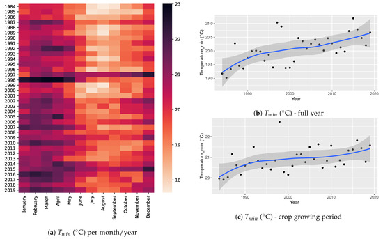
Figure 2.
Time series of average minimum temperature (°C) in Guayas from 1984 to 2019. (a) Heat-map of (°C) per each month and year. The color scale represents the temperature in °C. (b) (°C) averaged during the full year. (c) (°C) averaged during the maize crop growing period in Ecuador (January–May). Each dot represents one record, the blue line shows the smoothed time series and the shaded area represents the 95% confidence interval.
The fluctuated between 26 °C and over 33 °C, and the highest values occur during the dry season (June to November) of each year, similar to the other provinces. Notably, we note a significant increase in in Guayas from 2009; meanwhile, the lowest annual values were reported in 1997, 1998, and 1999. Moreover, an unusual warm growing period was observed in 2005 and 2007. shows a general increase. However, this change is greater during the wet season between January and May. The mean daily precipitation (mm) reaches the highest values during the wet season (January to May); the rest of the year, this province presents arid conditions (see Figure 2). The driest years were between 2005 and 2007. Concerning wind speed, the highest values are reported during the dry season in the second semester of each year, but they do not show any noticeable trend. Finally, the daily radiation values lie between 11.5 and 19.0 MJ m, noticing the higher values during the growing period.
The Mann–Kendall test identified a significant upward trend in during the full-year, crop growing period, and seasonal approach. Meanwhile, the has a significantly increasing trend in the full-year and seasonal analysis. Precipitation and wind speed do not have a significant trend and, the radiation (evaluated only until 2007) has a significantly negative trend in the seasonal Mann–Kendall test.
3.1.2. Los Rios
Maximum temperature records in Los Rios are shown in Figure 3. A similar analysis of the other climate parameters can be observed in Figure A5, Figure A6, Figure A7 and Figure A8.
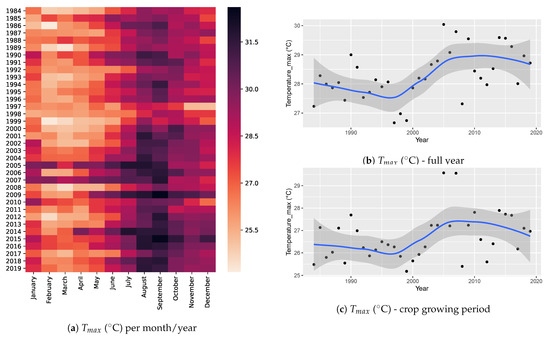
Figure 3.
Time series of average maximum temperature (°C) in Los Rios from 1984 to 2019. (a) Heat-map of (°C) per each month and year. The color scale represents the temperature in °C. (b) (°C) averaged during the full year. (c) (°C) averaged during the maize crop growing period in Ecuador (January–May). Each dot represents one record, the blue line shows the smoothed time series and the shaded area represents the 95% confidence interval.
According to the Mann–Kendall test, Los Rios has an upward trend in and in the full-year, crop growing period and seasonal approach. Moreover, during the year 1997, 1998, 2005, 2007, 2014, and 2015, an unusual temperature pattern was observed (see Figure 3 for minimum temperature). However, there is no significant trend for the precipitation and wind speed. Only stochastic changes can be noticed. On the other hand, the radiation showed a decreasing trend during the crop growing period, including the Mann–Kendall test’s seasonal approach.
3.1.3. Loja
The climate parameters fluctuations in Loja are shown in Figure A9, Figure A10, Figure A11 and Figure A12. An increasing trend in the values for the full year and growing period in Loja can be observed. This province shows lower and values than Guayas and Los Rios. Additionally, there are visible temperature anomalies for 2005, 2010 (high), and 1984, 1989 (low). In the last 15 years, Loja reported overall warmer than before 2005.
As for all studied provinces, the Loja precipitation has a high temporal variation (e.g., the wet period occurs during the earliest periods of record). Loja is the driest province between all provinces considered in this study, showing the lowest point in 2005 and 2007, and the higher before 2000 (see Figure 4).
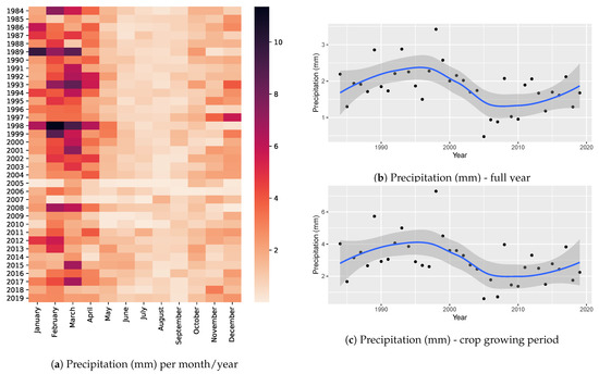
Figure 4.
Time series of daily average precipitation (mm) in Loja from 1984 to 2019. (a) Heat-map of daily precipitation (mm) per each month and year. The color scale represents the precipitation in mm. (b) Daily precipitation averaged during the full year. (c) Daily precipitation averaged during the maize crop growing period in Ecuador (January–May). Each dot represents one record, the blue line shows the smoothed time series and the shaded area represents the 95% confidence interval.
The Mann–Kendall test depicts Loja as the province with the most substantial evidence of climate change. During all the assessed periods (full-year, growing season, and seasonal), and values had a significant upward trend, while the precipitation had a downward trend. According to the seasonal Mann–Kendall, the wind speed had a drastic increasing trend, and the radiation values did not show any trend (between 1984 and 2007).
3.1.4. Manabi
A warmer period according to the climate variables and over the recent years is observed in Manabi (see Figure 5 for minimum temperature records). This change is more intensive during the dry season (June to December). Furthermore, unusual high values of occurred in 2005, 2007 and, of during 1997 and 1998. The precipitation was exceptionally high during 1997 and 1998. Regarding the wind speed, the fluctuation between the highest and lowest value, especially during the growing period, is low. Plots of the other climate parameters in Manabi are shown in the appendix section in Figure A13, Figure A14, Figure A15 and Figure A16.
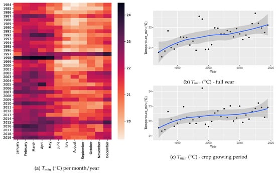
Figure 5.
Time series of average minimum temperature (°C) in Manabi from 1984 to 2019. (a) Heat-map of (°C) per each month and year. The color scale represents the temperature in °C. (b) (°C) averaged during the full year. (c) (°C) averaged during the maize crop growing period in Ecuador (January–May). Each dot represents one record, the blue line shows the smoothed time series and the shaded area represents the 95% confidence interval.
The Mann–Kendall test showed a significant monotonic upward trend in in all studied periods. Meanwhile, the had a significantly increasing trend in the full-year and seasonally, but not in the growing period. The radiation shows a significant downward trend in the full-year and seasonal approach. Moreover, the precipitation and wind speed did not present any significant trend.
3.1.5. Spatial Variability
We applied the Sen’s slope technique over our data series to know the magnitude of the trend previously calculated by the Mann–Kendall test. This analysis was done for the significant trend during the full-year period and during the crop growing period, summarized in Table 2. The magnitude of the significant trends during the crop growing period is essential because this will directly affect the maize yield, as shown in Section 3.3.
Table 2.
Summary of the Sen’s Slope test. The values represent the magnitude of the variation of each parameter per year. The sign + means a increasing trend, whereas − means a decreasing trend. The ns means “not significant” and refers to the lack of significant trend for that climate parameter. FY refers to the full year approach and GP refers to the crop growing period approach.
3.2. Calibration and Validation of the Model
The calibration was done for three of the most grown variety in Ecuador. Specifically, EMBLEMA is the most used in Guayas and Los Rios, DK7088 is widely grown in Loja, and TRIUNFO is largely used in Manabi. As a starting point for the calibration, we used the dataset for maize provide by the LINTUL5 model, and then, they were changed accordingly. Table 3 shows the final parameters configured for our calibration.
Table 3.
Adjusted values for crop parameters calibration of the model. The variety EMBLEMA was used in Guayas (G) and Los Rios (LR), DK7088 was used in Loja (L), and TRUENO was used in Manabi (M).
For validating the model, we simulate maize yield in the four provinces using the management data provided by literature references and the Ministry of Agriculture data since 2012. The simulation was done from 2002 to 2018 to compare the simulated yield with observed yield reported for the Ministry of Agriculture of Ecuador [38,39].
Figure 6 shows the simulated yields against the observed yield in Guayas (a) and Los Rios (b), Loja (a) and Manabi (b). The relative mean error (MR) of the averaged simulated yield in relation with the averaged observed yield from 2002 to 2018 was of ( Mg ha, Mg ha) in Guayas, ( Mg ha, Mg ha) in Los Rios, ( Mg ha, 3.9 Mg ha) in Loja and, ( Mg ha, Mg ha) in Manabi. However, for the evaluation of the model it is better to look at the standard deviation of the residuals.
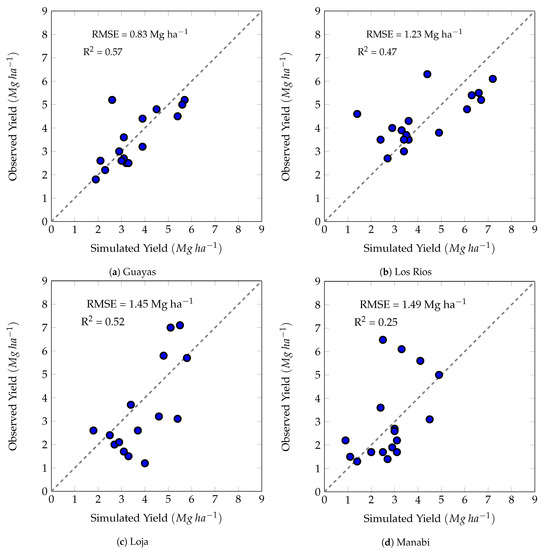
Figure 6.
Observed vs. Simulated Yields (Mg ha) from 2002 to 2018 in (a) Guayas, (b) Los Rios, (c) Loja and, (d) Manabi.
3.3. Climate Change Effects over Maize Yield
After the calibration of the model, we ran simulations on the four studied provinces. We used different amounts of nitrogen in our simulations to realistically represent the yield under rainfed and fertilizer conditions.
We applied the linear regression analysis in all the simulated yields to obtain the corresponding fitted values (trend) and each one’s slope. The slope is considered a combined effect of soil fertility and climate change at a lower rate of nitrogen application (<150 kg N ha), whereas the slope at a high rate of nitrogen application (>150 kg N ha) may be considered mainly an effect of climate change.
Figure 7 shows, for Guayas (a), Los Rios (b), Loja (c), and Manabi (d), the slopes of the trends of the simulated yields under different scenarios of Nitrogen application (a). We can see that in Guayas and Los Rios (Figure 7a,b) at lower rates of nitrogen application, the trend is negative. On the other hand, while more nitrogen is applied, the slope becomes zero.
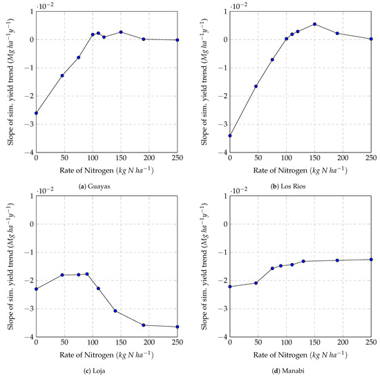
Figure 7.
The slopes of the simulated yield trends under different rates of Nitrogen application for (a) Guayas, (b) Los Rios, (c) Loja and (d) Manabi. Each dot represents the value of the slope (Mg ha year) of each scenario of nitrogen application. At lower rates of nitrogen application (<150), the effect is due to the loss of soil fertility and climate change and, at higher rates of nitrogen application (>150), the effect is mainly due to climate change.
As shown in Figure 7c, the negative impact increases in the semi-arid province Loja for more significant amounts of nitrogen application. At 100 kg N ha, the long-term decreased effect is roughly 0.02 Mg ha per year, and it is about Mg ha (negative) per year, when 250 kg N ha is applied.
Figure 7d shows the contrasting effects in Manabi province. Results show more significant negative effects at lower levels of Nitrogen application. For a higher N ratio, the effects become smaller (in magnitude) but are still negative. It shows a decreasing effect of N application and climate change on maize yield. Low values in Manabi are due to substantial yield underestimation by the model in 2016 and 2017.
3.4. Climate Change Effects on the Phenology
The effects of climate change on the length of the growing period were assessed in the simulated yields. The period 1984 to 2001 was taken as a baseline to compare with the period after 2002 until 2019. The non-parametric test Wilcox was used to find whether the difference in the median was significant or not. The results of each simulation unit were paired for these two periods.
Figure 8 shows the boxplots of the length of the growing period before 2001 and after 2002 in Guayas (a) and Los Rios (b), Loja (a), and Manabi (b). In Guayas, the median before 2001 was 128 days, and 125 days after 2002 (3 days less). The interquartile range (IQR) was 11.8 days before 2001 and 10.2 days after 2002. In Los Rios, the median before 2001 was 170 days (), and in the period after 2002 was 162 days (). In Loja, the median was 117 days () before 2001 and 109 days () after 2002. In Manabi, the median of the period before 2001 was 129 days (), while the period after 2002 had a median of 126 days (). The Wilcox text for the difference in the length of the growing period in all four provinces was highly significant ().
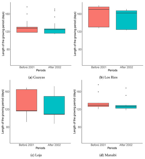
Figure 8.
Boxplot of the simulated length of crop growing period (days)—period from sowing to maturity—of each simulation unit in (a) Guayas, (b) Los Rios, (c) Loja and (d) Manabi. The red column shows the average from 1984 to 2001 of each simulation unit and the green column shows the average from 2002 to 2019 of each simulation unit for (a) Guayas, (b) Los Rios, (c) Loja and (d) Manabi.
4. Discussion
This study aims to assess recent climate change effects on the maize yield in different Ecuador provinces. One of them belongs to a semi-arid region. Our first hypothesis is the existence of climate change in the provinces of primary maize production.
4.1. Climate Change
Our results show that provinces in spatial proximity do not necessarily exhibit similar climate behavior, showing that location-specific climate data must be examined case by case. However, there are some similarities, such as the pattern in the precipitation concentrated between January and May. Previous works also confirm this finding [41]. A reason for this seasonality variation may be the Hadley circulation effect (Ecuador is part of the South Hadley cell). These cells are the low-latitude overturning circulations, where the air rises at the equator and sinks at approximately 30° latitude. It has seasonal variability, and it is dynamic [42]. All these seasonality variations cause a greater rainfall in the wet season. Therefore, farmers choose this season as they do not have access to an irrigation system to grow short term crops like maize [12].
The climate parameters in the coastal provinces (Guayas, Los Rios, and Manabi) are characterized by high temperatures and enough precipitation and radiation to grow maize. However, some unusual patterns were found during the years 1997, 1998. In this period, high temperatures, high precipitation (from November 1997 to June 1998), low wind speed and, high radiation were reported. Some of the described effects are characteristics of the el Niño phenomena [43].
Institutions in charge of monitoring the climate reported peaks in the rainfall patterns in 1997 and 1998 and classified them as an El Niño phenomenon. Furthermore, other works [44,45] used the ICEN index (Coastal El Niño Index, Indice Costero El Niño) and ONI index (Oceanic Niño Index), respectively, to confirm the presence of this phenomenon in the years 1997 and 1998. The United Nations Office for the Coordination of Humanitarian Affairs reports some negative impacts in agriculture due to this increase in rainfall. Thus, El Niño directly affected provinces in Ecuador’s coastal plain like Guayas, Los Rios, and Manabi [46].
Meanwhile, the La Niña phenomenon, which is characterized by frigid ocean temperatures in the Equatorial Pacific, tends to have an opposite impact than El Niño. It has been observed that La Niña had a strong impact during 1988–1989 and, with moderate effects during 1999, 2000, 2007, 2010 [47]. However, our results only show an impact on the precipitation (notably less) in 2007 for all provinces and anomalies in Loja temperature in 1988–1989. Nevertheless, a study [48] found that the drought in the Amazon basin caused the dry period in 2005 in Loja.
Our results also showed considerable differences in the climate patterns among the studied provinces. A possible explanation for this is the elevation gradients, which control the spatial and temporal variability of climate and greatly influence atmospheric circulation mechanisms among the country. These topographic differences could cause notable precipitation variability among the provinces even within a short distance [48].
The results of this study show a significant upward trend in temperature in all the provinces. These results are consistent with the findings in previous studies [4]. The authors used some data from meteorological stations of National Institute of Meteorology and Hydrology of Ecuador (INHAMI) to determine the temperature and precipitation trend of Ecuador from 1966 to 2011. They concluded that the minimum temperature had a strong trend of increase in the coastal provinces. The trends in maximum temperature showed a spatial variability, and the precipitation did not show a trend in the coastal region, but there were different effects in the precipitation among the whole country. However, in the provinces of the Highlands, they found an increasing trend in precipitation. That result differs from our findings in Loja, which belongs to the Highlands provinces. This difference could be due to the studied period and also due to the different considered locations. Contrary to us, their study is biased to stations located to the north, and Loja is indeed placed more to the south. Nevertheless, other authors found a declining trend in precipitation in the coast [49] and in some meteorological stations of the highlands [50].
The evidence of climate change in Ecuador was also mentioned by the Working Group II into the Fourth Assessment Report-WGII AR4 [3]. They found unusual extreme weather events in Latin America, and the mean increasing temperature trend was about 0.1 °C per decade. They also predicted more prominent rainfall anomalies (upward or downward) and more frequent climate extremes events for the 21st century. Our results also show an increasing trend in temperature of about 0.3 °C per decade, but during the growing period.
There is a lack of studies about the trend in radiation and wind speed. Therefore, further research is required to show the actual trend in these critical parameters for crop development. However, at a global scale, some studies showed a decreasing trend in solar radiation of about 1.4–2.7% per decade [51].
4.2. Effects of Climate Change over Maize Yield
Once the existence of recent climatic change has been proved, the impact on maize yields were investigated. This study’s results show significant effects on maize yield in Loja and Manabi, but not in Guayas and Los Rios. The effects of the recent climate change on maize yield in Ecuador have not been widely studied. An available study [10] showed that the changes in climate and environment had caused a shift in the establishment of maize croplands. Some maize farmers have started cultivating maize at higher altitudes in the Andes to compensate for the increase in temperature in the lower regions.
Our results concerning the yield changes in Guayas are shown in Figure 7. We can observe that at the lower amount of fertilizer application, the yield decreased from 1984 to 2019. Contrary, at greater rates of nitrogen, the trend became roughly zero. This unexpected result is plausible since Guayas is the less affected province by climate change (only the has a significant decrease). The decreased trend of the yields at lower rates of nitrogen could be due to loss of nutrients (mainly nitrogen) and a loss of soil fertility. This lack of nutrient availability affects crop growth. Our findings were also found in the study conducted by Chen et al. (2017) [52], who has found that at zero nitrogen application, the maize yield reduces in the long-term.
A similar scenario is shown in Los Rios province (Figure 7). However, those results were unforeseen because this province showed a significant warming climate in both , and a downward trend in radiation. One explanation may be that these temperatures were not critical in the critical stages of development (e.g., near to anthesis). Additionally, the range of temperatures has never exceeded 30 °C, set as maximum temperature for the emergence and as optimum temperature for crop growth in the model. Other authors also found this value as the upper maximum of the optimum temperature [53,54].
Regarding the radiation, it is well known that this parameter is a driver for photosynthesis and biomass growth in plant organs. Therefore, we could expect a decrease in the yield in Los Rios due to the downward trend in radiation, like some studies, previously reported [51,55]. However, the genotype could play a crucial role in decreasing radiation-sensitive [51], such as shading conditions and light use efficiency characteristics for each crop. The variety properties may explain the non-existing effect of the decreasing trend in radiation on yield in Los Rios since the variety used in Guayas and Los Rios (EMBLEMA) was calibrated at high radiation use efficiency values. This is different from other maize varieties used in Nigeria [56], and Etiophia [57], in which a lower radiation use efficiency in all the development stages was set up. Since the variety simulated was the same for Guayas and Los Rios, further research can be done taking into account this condition to have a more profound knowledge of the adaptability of this variety to the decrease of radiation.
The climate change effect in Manabi can be seen in Figure 7. Despite the increasing of Nitrogen application the yield trend still remains negative ( Mg ha per year at 250 kg N ha). It can confirm the hypothesis of the evidence of climate change on maize yield in Manabi. This province showed an increasing trend in the temperature, decreasing trend in radiation, and a greater compared to the other provinces. Although the temperature range in Manabi does not exceed the critical temperature, the mixture of temperature and radiation could explain the yield changes. On the one hand, the increase in the temperature reduces the length of the growing period. On the other hand, decreasing radiation affects the growth rate. This finding agrees with the study conducted by Shi et al. (2014) [58] who investigated maize yield’s vulnerability to climate change in Africa during 1961–2010. They found that each 1 °C of mean temperature increase resulted in yield losses of over 10% in eight countries and 5–10% in 10 countries of Africa.
An even more interesting finding is the impact of climate change in the semi-arid province Loja. Here, at high rates of applied nitrogen, the yield shows a clear downward trend, as can be seen in Figure 7. In this province, not only the , had an increasing trend during the growing period, but the precipitation also decreased due to climate change. Furthermore, this province is the driest compared with all the studied provinces. The water stress could explain the decrease in the yield in recent years that the maize suffered. These events are more frequent after 2005. According to the simulated yield results, the water stress was particularly critical in the phase of anthesis. Moreover, this more substantial decrease at high nitrogen application rates could be explained by the higher potential transpiration demand caused by higher temperatures and higher LAI levels [59,60]. At lower levels of nitrogen application, the LAI decreased due to nutrient deficiency, and the potential crop water demand is lower than at higher which occurs at higher levels of nitrogen application (LAI). A greater LAI needs more water, and the potential crop transpiration increases. It caused water stress and corresponding yield reduction that can be noticed clearly at large amounts of nitrogen. The combined trends in precipitation (decreasing) and temperature (increasing) might have caused a more substantial reduction of the yield due to a shorted crop growing period [61], which was about eight days less in the period after 2002, according to our results.
Additionally, the changes mentioned above in Loja (more temperature and less precipitation) could affect the soil moisture available for the crop uptake due to an increase in soil evaporation. Parry et al. (1990) [61] reported that at mid-latitudes, evaporation increases roughly 5% for each °C of mean annual temperature. A strongly positive relationship between lack of water availability and temperature can be seen in the results. It is also mentioned in Reddy (2015) [62], in a dry zone of the Volga Basin, where an increasing change of 0.5–1 °C without a change in precipitation had little effect on spring-wheat yield, while a decrease of 20% in precipitation (with the exact change in temperature) reduce yields by approximately 10%.
4.3. Climate Change Effects on Phenology
We found a significantly longer length of crop growing period in all provinces from 1984 to 2001 compared with the period from 2002 to 2019. This change may be explained by the significant increase in temperature that all the provinces showed. Each development stage’s length is a function of the cumulative daily effective temperature, which is the average temperature above a crop-specific base temperature. In our study, the base temperature was set to 8 °C. Thus, when the temperature increases, this heat sum is achieved in less time, and the maturity is reached faster. Furthermore, a study [61] mentions that temperature increase shortens the reproductive phase, limiting the canopy’s duration and consequently, the period for the interception of light (with the canopy) to produce biomass reduces, as well.
However, our study shows that the length of the crop growing period differs across each province. The variability of this duration in Los Rios and Loja is greater than in Guayas and Manabi. It may be explained by the differences in elevation and mean temperature over the growing period in these provinces.
Spatial variability in length of growing period (LGP) was also found by Vrieling et al. (2013) [63], who studied this parameter from 1981 to 2011 in Africa. They found high variability in LGP in arid and semi-arid zones. Significant negative trends in LGP were also depicted in Tanzania, north of Mozambique, and North of the Sahel. In our study, Loja, considered a province with a predominantly semi-arid climate, showed significant variability.
4.4. Uncertainties of the Methodology
In simulation studies, some uncertainties may cause differences between reality and simulation output. We use inputs such as climate data, soil properties, crop variety properties, and management information. The radiation was not taken from the same source in the total time-span by Nasa Power, which could cause a relevant break in the time series.
In our study, the field observations used to calibrate the model contained only phenology and final grain yield observations. There was a lack of information about sequential measurements of biomass, leaf area index, and observed soil properties. This limitation in the calibration could be one reason for the values of RMSE shown in Figure 6 for the validation of the model at province scale.
Finally, the decrease of the yield in a particular year could be due to pests or diseases, but LINTUL5 cannot include them in the final simulated yield.
5. Conclusions
Our study’s objective was to assess whereas the recent climate change had an impact on the historical maize yields in four provinces of Ecuador using a crop modelling approach. The results showed that the crop model LINTUL5 performed better in Guayas, Los Rios, and Loja, but it did not fit Manabi accurately ( Mg ha). The accuracy of the model performance may be enhanced using more precise information of the soil, weather, and management practices during the calibration. Regarding the climate change impact on maize yield, our counterfactual yield results showed a lack of effects in Guayas and Los Rios, but a loss yield in the semi-arid province Loja. The crop growing period length was shortened in all provinces. Our study has evaluated the applicability of the model LINTUL5 (embedded into the SIMPLACE modelling framework) using high-resolution climate data for estimating the effect of climate change on maize yield in the provinces of primary maize production of Ecuador. Further studies are necessary to investigate the impact of climate change in future scenarios.
Author Contributions
Conceptualization, A.S., G.L. and T.G.; Methodology, A.S., G.L. and T.G.; Software, G.L.; Validation, A.S.; Formal Analysis, G.L.; Writing—Original Draft Preparation, G.L.; Writing—Review and Editing, A.S., T.G., F.E. All authors have read and agreed to the published version of the manuscript.
Funding
This study was funded by Federal Ministry of Education and Research (BMBF) of Germany. Furthermore, this work was partly funded by the Deutsche Forschungsgemeinschaft (DFG, German Research Foundation) under Germany’s Excellence Strategy—EXC 2070—390732324 (PhenoRob) and by the German Federal Ministry of Education and Research (BMBF) in the framework of the funding measure ‘Soil as a Sustainable Resource for the Bioeconomy—BonaRes’, project BonaRes (Module A): BonaRes Center for Soil Research, subproject ‘Sustainable SubsoilManagement—Soil3’ (grant 031B0151A).
Institutional Review Board Statement
Not applicable.
Informed Consent Statement
Not applicable.
Acknowledgments
We would like to thank Andreas Enders and Gunther Krauss for their support in SIMPLACE framework.Climate data were obtained from the NASA Langley Research Center (LaRC) POWER Project funded through the NASA Earth Science/Applied Science Program.
Conflicts of Interest
The authors declare no conflict of interest.
Appendix A. Mann–Kendall Trend Test
The Mann–Kendall trend test is based on the correlation between the values of an ordered time series, and it is conducted as follows [64]:
- The data must be sorted in the order in which they were collected over time, , which denote the measurements obtained at times , respectively.
- Determine the sign of all possible differences , where . These differences are .
- Let be an indicator function that takes on the values 1, 0, or according to the sign of , that is,
Then the Mann–Kendall Score (S) is compute as Equation (A2) shows.
If S is a positive number, observations obtained later in time tend to be larger than observations made earlier. If S is a negative number, then observations made later in time tend to be smaller than observations made earlier [64].
Appendix B. Climate Parameters in Guayas, Los Rios, Loja and Manabi
Appendix B.1. Guayas

Figure A1.
Time series of average maximum temperature (°C) in Guayas from 1984 to 2019. (a) Heat-map of (°C) per each month and year. The color scale represents the temperature in °C. (b) (°C) averaged during the full year. (c) (°C) averaged during the maize crop growing period in Ecuador (January–May). Each dot represents one record, the blue line shows the smoothed time series and the shaded area represents the 95% confidence interval.


Figure A2.
Time series of daily average precipitation (mm) in Guayas from 1984 to 2019. (a) Heat-map of daily precipitation (mm) per each month and year. The color scale represents the precipitation in mm. (b) Daily precipitation averaged during the full year. (c) Daily precipitation averaged during the maize crop growing period in Ecuador (January–May). Each dot represents one record, the blue line shows the smoothed time series and the shaded area represents the 95% confidence interval.


Figure A3.
Time series of average wind speed (m s) in Guayas from 1984 to 2019. (a) Heat-map of wind speed (m s) per each month and year. The color scale represents the wind speed in m s. (b) Wind speed averaged during the full year. (c) Wind speed averaged during the maize crop growing period in Ecuador (January–May). Each dot represents one record, the blue line shows the smoothed time series and the shaded area represents the 95% confidence interval.


Figure A4.
Time series of average radiation (MJ m) in Guayas. (a) Heat-map of radiation (MJ m) per each month and year from 1984 to 2019. The color scale represents the radiation (MJ m). (b) Radiation averaged during the full year from 1984 to 2007. (c) Radiation averaged during the maize crop growing period in Ecuador (January–May) from 1984 to 2007. Each dot represents one record, the blue line shows the smoothed time series and the shaded area represents the 95% confidence interval.

Appendix B.2. Los Rios

Figure A5.
Time series of average minimum temperature (°C) in Los Rios from 1984 to 2019. (a) Heat-map of (°C) per each month and year. The color scale represents the temperature in °C. (b) (°C) averaged during the full year. (c) (°C) averaged during the maize crop growing period in Ecuador (January–May). Each dot represents one record, the blue line shows the smoothed time series and the shaded area represents the 95% confidence interval.


Figure A6.
Time series of daily average precipitation (mm) in Los Rios from 1984 to 2019. (a) Heat-map of daily precipitation (mm) per each month and year. The color scale represents the precipitation in mm. (b) Daily precipitation averaged during the full year. (c) Daily precipitation averaged during the maize crop growing period in Ecuador (January–May). Each dot represents one record, the blue line shows the smoothed time series and the shaded area represents the 95% confidence interval.


Figure A7.
Time series of average wind speed (m s) in Los Rios from 1984 to 2019. (a) Heat-map of wind speed (m s) per each month and year. The color scale represents the wind speed in m s. (b) Wind speed averaged during the full year. (c) Wind speed averaged during the maize crop growing period in Ecuador (January–May). Each dot represents one record, the blue line shows the smoothed time series and the shaded area represents the 95% confidence interval.


Figure A8.
Time series of average radiation (MJ m) in Los Rios. (a) Heat-map of radiation (MJ m) per each month and year from 1984 to 2019. The color scale represents the radiation (MJ m). (b) Radiation averaged during the full year from 1984 to 2007. (c) Radiation averaged during the maize crop growing period in Ecuador (January–May) from 1984 to 2007. Each dot represents one record, the blue line shows the smoothed time series and the shaded area represents the 95% confidence interval.

Appendix B.3. Loja

Figure A9.
Time series of average maximum temperature (°C) in Loja from 1984 to 2019. (a) Heat-map of (°C) per each month and year. The color scale represents the temperature in °C. (b) (°C) averaged during the full year. (c) (°C) averaged during the maize crop growing period in Ecuador (January–May). Each dot represents one record, the blue line shows the smoothed time series and the shaded area represents the 95% confidence interval.


Figure A10.
Time series of average minimum temperature (°C) in Loja from 1984 to 2019. (a) Heat-map of (°C) per each month and year. The color scale represents the temperature in °C. (b) (°C) averaged during the full year. (c) (°C) averaged during the maize crop growing period in Ecuador (January–May). Each dot represents one record, the blue line shows the smoothed time series and the shaded area represents the 95% confidence interval.


Figure A11.
Time series of average wind speed (m s) in Loja from 1984 to 2019. (a) Heat-map of wind speed (m s) per each month and year. The color scale represents the wind speed in m s. (b) Wind speed averaged during the full year. (c) Wind speed averaged during the maize crop growing period in Ecuador (January–May). Each dot represents one record, the blue line shows the smoothed time series and the shaded area represents the 95% confidence interval.


Figure A12.
Time series of average radiation (MJ m) in Loja. (a) Heat-map of radiation (MJ m) per each month and year from 1984 to 2019. The color scale represents the radiation (MJ m). (b) Radiation averaged during the full year from 1984 to 2007. (c) Radiation averaged during the maize crop growing period in Ecuador (January–May) from 1984 to 2007. Each dot represents one record, the blue line shows the smoothed time series and the shaded area represents the 95% confidence interval.

Appendix B.4. Manabi

Figure A13.
Time series of average maximum temperature (°C) in Manabi from 1984 to 2019. (a) Heat-map of (°C) per each month and year. The color scale represents the temperature in °C. (b) (°C) averaged during the full year. (c) (°C) averaged during the maize crop growing period in Ecuador (January–May). Each dot represents one record, the blue line shows the smoothed time series and the shaded area represents the 95% confidence interval.


Figure A14.
Time series of daily average precipitation (mm) in Manabi from 1984 to 2019. (a) Heat-map of daily precipitation (mm) per each month and year. The color scale represents the precipitation in mm. (b) Daily precipitation averaged during the full year. (c) Daily precipitation averaged during the maize crop growing period in Ecuador (January–May). Each dot represents one record, the blue line shows the smoothed time series and the shaded area represents the 95% confidence interval.


Figure A15.
Time series of average wind speed (m s) in Manabi from 1984 to 2019. (a) Heat-map of wind speed (m s) per each month and year. The color scale represents the wind speed in m s. (b) Wind speed averaged during the full year. (c) Wind speed averaged during the maize crop growing period in Ecuador (January–May). Each dot represents one record, the blue line shows the smoothed time series and the shaded area represents the 95% confidence interval.


Figure A16.
Time series of average radiation (MJ m) in Manabi. (a) Heat-map of radiation (MJ m) per each month and year from 1984 to 2019. The color scale represents the radiation (MJ m). (b) Radiation averaged during the full year from 1984 to 2007. (c) Radiation averaged during the maize crop growing period in Ecuador (January–May) from 1984 to 2007. Each dot represents one record, the blue line shows the smoothed time series and the shaded area represents the 95% confidence interval.

References
- World-Bank. Agriculture, Forestry, and Fishing, Value Added (% of GDP)\Data. 2020. Available online: https://data.worldbank.org/indicator/NV.AGR.TOTL.ZS (accessed on 25 February 2020).
- MAG. General Information of Agriculture-Ecuador. 2020. Available online: https://www.g-fras.org/en/world-wide-extension-study/south-america/south-america/ecuador.html (accessed on 25 February 2020).
- IPCC. Chapter: Central and South America. In AR5 Climate Change 2014: Impacts, Adaptation, and Vulnerability; 2014; p. 68. Available online: https://www.ipcc.ch/report/ar5/wg2/ (accessed on 25 February 2020).
- Morán-Tejeda, E.; Bazo, J.; López-Moreno, J.I.; Aguilar, E.; Azorín-Molina, C.; Sanchez-Lorenzo, A.; Martínez, R.; Nieto, J.J.; Mejía, R.; Martín-Hernández, N.; et al. Climate trends and variability in Ecuador (1966–2011). Int. J. Climatol. 2016, 36, 3839–3855. [Google Scholar] [CrossRef]
- Burke, E.; Goldenson, N.; Moon, T.; Po-Chedley, S. Climate and Climate Change in Ecuador: An Overview. Atmos. Sci. 2009, 57. [Google Scholar]
- Ontaneda, G.; Caceres, L.; Mejia, R. Evidencias del Cambio Climático en Ecuador. Bulletin de l’Institut Français D’études Andines 1998, 27. [Google Scholar]
- Prăvălie, R. Recent changes in global drylands_ Evidences from two major aridity databases. Catena 2019, 178, 209–231. [Google Scholar] [CrossRef]
- FAO. Trees, Forests and Land Use in Drylands: The First Global Assessment—Full Report. Technical Report. 2019. Available online: https://www.google.com.hk/url?sa=t&rct=j&q=&esrc=s&source=web&cd=&cad=rja&uact=8&ved=2ahUKEwj7hsKkn4fvAhWrIqYKHSo_DIgQFjAAegQIAhAD&url=http%3A%2F%2Fwww.fao.org%2F3%2Fca7148en%2Fca7148en.pdf&usg=AOvVaw16GV9LfxEo9eAfZTGgL6Nh (accessed on 25 February 2020).
- Fries, A.; Silva, K.; Pucha-Cofrep, F.; Oñate-Valdivieso, F.; Ochoa-Cueva, P. Water Balance and Soil Moisture Deficit of Different Vegetation Units under Semiarid Conditions in the Andes of Southern Ecuador. Climate 2020, 8, 30. [Google Scholar] [CrossRef]
- Skarbø, K.; VanderMolen, K. Maize migration: Key crop expands to higher altitudes under climate change in the Andes. Clim. Dev. 2016, 8, 245–255. [Google Scholar] [CrossRef]
- Carvajal Calderón, M. Impactos de la Variabilidad y el Cambio Climático Sobre el Cultivo de Banano (Musa Spp) en Tres Países Productores de América Latina. Bachelor Thesis, University Autónoma De Occidente, Cali, Colombia, 2016. [Google Scholar]
- MAG. Rendimiento Informe de Maíz 2019. 2019. Available online: https://www.google.com.hk/url?sa=t&rct=j&q=&esrc=s&source=web&cd=&cad=rja&uact=8&ved=2ahUKEwis88HXn4fvAhUKyosBHU-_CxwQFjAAegQIARAD&url=http%3A%2F%2Fwww.mag.go.cr%2Fbibliotecavirtual%2FF01-4042.pdf&usg=AOvVaw3lDBh5aDKFrJoKcccgcUCL (accessed on 25 February 2020).
- Lobell, D.B.; Schlenker, W.; Costa-Roberts, J. Climate Trends and Global Crop Production Since 1980. Science 2011, 333, 616–620. [Google Scholar] [CrossRef] [PubMed]
- INEC. Features of Provinces in Ecuador. 2019. Available online: https://www.inec.cr/ (accessed on 25 February 2020).
- Climate-Data.org. Clima Guayas: Temperatura, Climograma y Tabla Climática Para Guayas—Climate-Data.Org. 2019. Available online: https://es.climate-data.org/america-del-sur/ecuador/provincia-del-guayas/guayaquil-2962/ (accessed on 25 February 2020).
- Moreno, J.; Sevillano, G.; Valverde, O.; Loayza, V.; Haro, R.; Zambrano, J. Soil from the Coastal Plane. In The Soils of Ecuador; World Soils Book Series; Springer: Berlin/Heidelberg, Germany, 2018. [Google Scholar]
- Eglitis-Media. Climate in Manabí, Ecuador. 2020. Available online: https://www.worlddata.info/america/ecuador/climate-manabi.php (accessed on 25 February 2020).
- Moreno, J.; Bernal, G.; Espinoza, J. Introduction. In The Soils of Ecuador; World Soils Book Series; Springer: Berlin/Heidelberg, Germany, 2018. [Google Scholar]
- Climate-Data.org. Clima Los Rios: Temperatura, Climograma y Tabla Climática Para Guayas—Climate-Data.org. 2019. Available online: https://es.climate-data.org/america-del-sur/ecuador-63/ (accessed on 25 February 2020).
- Climate-Data.org. Clima Loja: Temperatura, Climograma y Tabla climática para Guayas—Climate-Data.org. 2019. Available online: https://es.climate-data.org/america-del-sur/ecuador-63/ (accessed on 25 February 2020).
- NASA POWER. POWER Data Access Viewer; 2020. Available online: https://power.larc.nasa.gov/ (accessed on 25 February 2020).
- Stackhouse, P.W.; Zhang, T.; Westberg, D.; Barnett, A.J.; Bristow, T.; Macpherson, B.; Hoell, J.M. POWER Release 8.0.1 (with GIS Applications) Methodology (Data Parameters, Sources, & Validation) Documentation Date December 12, 2018 (All previous versions are obsolete) (Data Version 8.0.1; Web Site Version 1.1.0); 2018; p. 99. Available online: https://power.larc.nasa.gov/documents/POWER_Data_v8_methodology.pdf (accessed on 25 February 2020).
- ISRIC. SoilGrids—Global Gridded Soil Information. 2020. Available online: https://www.isric.org/explore/soilgrids (accessed on 25 February 2020).
- Rawls, W.; Ahuja, L.; Maidment, D. Handbook of Hydrology; McGraw-Hill: New York, NY, USA, 1993. [Google Scholar]
- Atta-ur-Rahman; Dawood, M. Spatio-statistical analysis of temperature fluctuation using Mann–Kendall and Sen’s slope approach. Clim. Dyn. 2017, 48, 783–797. [Google Scholar] [CrossRef]
- Hamed, K.H. Trend detection in hydrologic data: The Mann–Kendall trend test under the scaling hypothesis. J. Hydrol. 2008, 349, 350–363. [Google Scholar] [CrossRef]
- Shibu, M.; Leffelaar, P.; van Keulen, H.; Aggarwal, P. LINTUL3, a simulation model for nitrogen-limited situations: Application to rice. Eur. J. Agron. 2010, 32, 255–271. [Google Scholar] [CrossRef]
- Wolf, J. LINTUL5: Simple Generic Model for Simulation of Crop Growth under Potential, Water Limited and Nitrogen, Phosphorus and Potassium Limited Conditions; Technical Report; Wageningen UR: Wageningen, The Netherlands, 2012. [Google Scholar]
- Srivastava, A.K.; Ceglar, A.; Zeng, W.; Gaiser, T.; Mboh, C.M.; Ewert, F. The Implication of Different Sets of Climate Variables on Regional Maize Yield Simulations. Atmosphere 2020, 11, 180. [Google Scholar] [CrossRef]
- Gabaldón-Leal, C.; Webber, H.; Otegui, M.E.; Slafer, G.A.; Ordóñez, R.A.; Gaiser, T.; Lorite, I.J.; Ruiz-Ramos, M.; Ewert, F. Modelling the impact of heat stress on maize yield formation. Field Crops Res. 2016, 198, 226–237. [Google Scholar] [CrossRef]
- Srivastava, A.K.; Gaiser, T.; Paeth, H.; Ewert, F. The impact of climate change on Yam (Dioscorea alata) yield in the savanna zone of West Africa. Agric. Ecosyst. Environ. 2012, 153, 57–64. [Google Scholar] [CrossRef]
- SIMPLACE. SlimWater Simplace Documentation. 2019. Available online: https://simplace.ipf.uni-bonn.de/doc/4.2/simplace_run/class_net.simplace.usermodules.thomas.SlimWater.html (accessed on 25 February 2020).
- SIMPLACE. SoilCN Simplace Documentation. 2019. Available online: https://simplace.net/doc/simplace_modules/class_net.simplace.sim.components.soil.soilcn.SoilCN.html (accessed on 25 February 2020).
- Campuzano, M. Evaluación del Comportamiento Agronómico de dos Híbridosexperimentales Promisorio de Maíz en Tres Localidades del Litoralecuatoriano y Una en los Valles sub Tropicales de la Provincia de Loja. Bachelor Thesis, Universidad Técnica de Babahoyo, Babahoyo, Ecuador, 2019. [Google Scholar]
- Toledo Ronquillo, B. Evaluación Agronómica de dos Híbridos de Maíz (Zea Mays L.) en Condición de Siembras Comerciales, en la Granja Experimental “Limoncito”, en época Lluviosa. Bachelor Thesis, Universidad Católica de Santiago de Guayaquil, Guayaquil, Ecuador, 2017. [Google Scholar]
- Bayas Silva, M.; Castillo Vera, H. Determinación de la Respuesta de Cuatro Enraizantes Aplicados Sobre la Semilla de Maíz (Zea Maíz) del Hibrido Dekalb 7088 en época Lluviosa en la Zona de Febres Cordero—Los Ríos. Bachelor Thesis, Universidad Técnica Estatal de Quevedo, Quevedo, Ecuador, 2014. [Google Scholar]
- Boogaard, H.L.; Diepen, C.A.v.; Rotter, R.P.; Cabrera, J.M.C.A.; Laar, H.H.v. WOFOST 7.1; User’s Guide for the WOFOST 7.1 Crop Growth Simulation Model and WOFOST Control Center 1.5; Technical Report 52; SC-DLO: Wageningen, The Netherlands, 1998. [Google Scholar]
- Borbor-Cordova, M.J.; Boyer, E.W.; McDowell, W.H.; Hall, C.A. Nitrogen and phosphorus budgets for a tropical watershed impacted by agricultural land use: Guayas, Ecuador. Biogeochemistry 2006, 79, 135–161. [Google Scholar] [CrossRef]
- MAG. Reports of Maize Yield in Ecuador. 2019. Available online: https://www.statista.com/statistics/955406/ecuador-corn-production-volume/ (accessed on 25 February 2020).
- MAG. Technical Report of Maize (Zea Mays L.) Crop in Ecuador. 2020. Available online: https://www.statista.com/statistics/955406/ecuador-corn-production-volume/ (accessed on 25 February 2020).
- Vicente-Serrano, S.M.; Aguilar, E.; Martínez, R.; Martín-Hernández, N.; Azorin-Molina, C.; Sanchez-Lorenzo, A.; El Kenawy, A.; Tomás-Burguera, M.; Moran-Tejeda, E.; López-Moreno, J.I.; et al. The complex influence of ENSO on droughts in Ecuador. Clim. Dyn. 2017, 48, 405–427. [Google Scholar] [CrossRef]
- Piana, M. Hadley Cells. 2020. Available online: https://www.seas.harvard.edu/climate/eli/research/equable/hadley2.html (accessed on 25 February 2020).
- NOAA. What is El Niño?\El Nino Theme Page—A Comprehensive Resource; 2020. Available online: https://www.pmel.noaa.gov/elnino/ (accessed on 25 February 2020).
- ENFEN. Definición Operacional de los Eventos El Niño y La Niña y Sus Magnitudes en la Costa del Peru. Technical Report. 2012. Available online: https://www.dhn.mil.pe/nota_tecnica_enfen (accessed on 25 February 2020).
- NOAA. What is La Niña?\El Nino Theme Page—A Comprehensive Resource; 2020. Available online: https://www.pmel.noaa.gov/elnino/what-is-la-nina (accessed on 25 February 2020).
- OCHA. Ecuador El Niño Floods Situation Report No. 6—Ecuador. 1998. Available online: https://reliefweb.int/report/ecuador/ecuador-el-ni%C3%B1o-floods-situation-report-no-6 (accessed on 25 February 2020).
- NOAA. NOAA’s Climate Prediction Center; 2020. Available online: https://www.cpc.ncep.noaa.gov/ (accessed on 25 February 2020).
- Rollenbeck, R.; Bendix, J. Rainfall distribution in the Andes of southern Ecuador derived from blending weather radar data and meteorological field observations. Atmos. Res. 2011, 99, 277–289. [Google Scholar] [CrossRef]
- World-Bank. Vulnerability, Risk Reduction, and Adaptation to Climate Change ECUADOR. Technical Report. 2011. Available online: https://openknowledge.worldbank.org/handle/10986/12744 (accessed on 25 February 2020).
- Tobar, V.; Wyseure, G. Seasonal rainfall patterns classification, relationship to ENSO and rainfall trends in Ecuador. Int. J. Climatol. 2018, 38, 1808–1819. [Google Scholar] [CrossRef]
- Yang, Y.; Xu, W.; Hou, P.; Liu, G.; Liu, W.; Wang, Y.; Zhao, R.; Ming, B.; Xie, R.; Wang, K.; et al. Improving maize grain yield by matching maize growth and solar radiation. Sci. Rep. 2019, 9, 3635. [Google Scholar] [CrossRef] [PubMed]
- Chen, P.; Du, Q.; Liu, X.; Zhou, L.; Hussain, S.; Lei, L.; Song, C.; Wang, X.; Liu, W.; Yang, F.; et al. Effects of reduced nitrogen inputs on crop yield and nitrogen use efficiency in a long-term maize-soybean relay strip intercropping system. PLoS ONE 2017, 12. [Google Scholar] [CrossRef] [PubMed]
- Gilmore, E.C.; Rogers, J.S. Heat Units as a Method of Measuring Maturity in Corn1. Agron. J. 1958, 50, 611–615. [Google Scholar] [CrossRef]
- Tollenaar, M.; Daynard, T.B.; Hunter, R.B. Effect of Temperature on Rate of Leaf Appearance and Flowering Date in Maize1. Crop Sci. 1979, 19. [Google Scholar] [CrossRef]
- Tao, Z.Q.; Chen, Y.Q.; Li, C.; Zou, J.X.; Yan, P.; Yuan, S.F.; Wu, X.; Sui, P. The causes and impacts for heat stress in spring maize during grain filling in the North China Plain—A review. J. Integr. Agric. 2016, 15, 2677–2687. [Google Scholar] [CrossRef]
- Lopez, G.; Kolem, H.B.; Srivastava, A.K.; Gaiser, T.; Ewert, F. A Model-Based Estimation of Resource Use Efficiencies in Maize Production in Nigeria. Sustainability 2019, 11, 5114. [Google Scholar] [CrossRef]
- Srivastava, A.K.; Mboh, C.M.; Gaiser, T.; Kuhn, A.; Ermias, E.; Ewert, F. Effect of mineral fertilizer on rain water and radiation use efficiencies for maize yield and stover biomass productivity in Ethiopia. Agric. Syst. 2019, 168, 88–100. [Google Scholar] [CrossRef]
- Shi, W.; Tao, F. Vulnerability of African maize yield to climate change and variability during 1961–2010. Food Secur. 2014, 6, 471–481. [Google Scholar] [CrossRef]
- Kirschbaum, M.U.F.; McMillan, A.M.S. Warming and Elevated CO2 Have Opposing Influences on Transpiration. Which is more Important? Curr. For. Rep. 2018, 4, 51–71. [Google Scholar] [CrossRef]
- Stuart Chapin, F. 16—Functional Role of Growth Forms in Ecosystem and Global Processes. In Scaling Physiological Processes; Ehleringer, J.R., Field, C.B., Eds.; Physiological Ecology; Academic Press: San Diego, CA, USA, 1993; pp. 287–312. [Google Scholar] [CrossRef]
- Parry, M. Climate Change and World Agriculture; Earthscan Publications: London, UK, 1990. [Google Scholar]
- Reddy, P.P. Climate Resilient Agriculture for Ensuring Food Security; Springer: New Delhi, India, 2015. [Google Scholar] [CrossRef]
- Vrieling, A.; de Leeuw, J.; Said, M. Length of Growing Period over Africa: Variability and Trends from 30 Years of NDVI Time Series. Remote Sens. 2013, 5, 982–1000. [Google Scholar] [CrossRef]
- Gilbert, R. Statistical Methods for Environmental Pollution Monitoring; Wiley: New York, NY, USA, 1987. [Google Scholar]


Publisher’s Note: MDPI stays neutral with regard to jurisdictional claims in published maps and institutional affiliations. |
© 2021 by the authors. Licensee MDPI, Basel, Switzerland. This article is an open access article distributed under the terms and conditions of the Creative Commons Attribution (CC BY) license (http://creativecommons.org/licenses/by/4.0/).