Downscaling and Evaluation of Seasonal Climate Data for the European Power Sector

Abstract

Within the Clim2Power project, two case studies focus on seasonal variations of the hydropower production in the river basins of the Danube (Germany/Austria) and the Douro (Portugal). To deliver spatially highly resolved climate data as an input for the hydrological models, the forecasts of the German Climate Forecast System (GCFS2.0) need to be downscaled. The statistical-empirical method EPISODES is used in this approach. It is adapted to the seasonal data, which consists of ensemble hindcasts and forecasts. Beside this, the two case study regions need specific configurations of the statistical model, providing appropriate predictors for the meteorological variables. This paper describes the technical details of the adaptation of the EPISODES method for the needs of Clim2Power. We analyse the hindcast skill of the downscaled hindcasts of all four seasons for the two variables near-surface (2 m) temperature and precipitation, and conclude that on the average the skill is conserved compared to the global model. This means that the seasonal information is available at a higher spatial resolution without losing skill. Furthermore, the output of the statistical downscaling is nearly bias-free, which is, beside the higher spatial resolution, an added value for the climate service.

1. Introduction

Weather and climate influence renewable energy production on different time scales. The aim of the ERA-NET [1] project Clim2Power is to investigate climate driven changes in the European power system in the long-term (climate projections) and on a seasonal time scale [2]. To make the diversity of climate data useable for decision makers, a climate service was developed within Clim2Power. It addresses trading companies and power systems operators, but also managers and policy makers. A strong user engagement is essential to deliver tailored information to the end user. Thus, in a first step, communication scientists worked out the user needs, to define appropriate products.

Within the multidisciplinary consortium, different modelling groups simulate the production of wind, solar and hydro energy as well as electricity, heating and cooling demand. Traditional physical models as well as machine learning approaches are used to calculate capacity factors from meteorological data. They serve as input indicators for energy system and power models (e.g., TIMES, [3,4]) which calculate variations in the European power system and its impacts on electricity costs, power generation from renewable energy sources (RES), etc.

Beside the European wide study, the climate service is tested within four regional case studies in France, Sweden, Portugal, and Germany-Austria. The two latter also include hydrological modelling of the river basins of the Douro river and the Upper Danube, respectively. These two case studies focus on seasonal variations in the hydropower generation.

COSERO, a continuous, semi-distributed rainfall-runoff model developed at the University of Natural Resources and Life Science, Vienna [5] and the hydrologic modelling system HEC-HMS [6] both rely on spatially highly resolved meteorological input data, first of all near-surface temperature and precipitation. To obtain climatological time series of runoff, the regional reanalysis COSMO-REA6 [7] is suitable with a spatial resolution of 6 km. The models were tested on this data set, which was available from 1995 to 2015.

When it comes to seasonal forecasting, global earth system models can be run in special configurations to forecast deviations from a mean climate state of the next months. In those models, the components of the earth system-atmosphere, ocean and land surface are coupled. The physical processes of the ocean and the land surface react on longer time scales than those of the atmosphere and are subsequently sources of extended predictability. This allows forecasts beyond the limit of atmosphere-only weather forecasts [8,9,10].

Europe is one of the most challenging regions with regard to seasonal forecasting. Virtually all operationally performed coupled models show low skill over Europe, which itself depends also strongly on the target season. While Scaife et al. [11] could show that improving atmospheric processes as well as increasing the ocean resolution enhances the skill for the British Isles, significant improvement from the dynamical models over the European continent is still hard to get (compare also with [10]). Thus, some efforts were made to improve the forecast skill over Europe by using statistical-dynamical methods as ensemble subsampling based on teleconnections [12]. While this method is very successful in improving the winter forecasts, it depends very heavily on the forecast start time and is not applicable for each of the 12 forecast months.

In Clim2Power, the output of the coupled global German Climate Forecast System (GCFS2.0, [13]) is used to generate the forecasts of the meteorological variables for the seasons ahead. The system is run operationally at Deutscher Wetterdienst (DWD) since 2016 and is a joint development with the Max Planck Institute for Meteorology (MPI-M) and the Universität Hamburg (UHH). The GCFS2.0 has a spectral resolution of T127, which corresponds to about 70 km at 50° N. The spatial resolution has doubled compared to its former version GCFS1.0 but it is still too coarse for hydrological modelling. For this reason, a downscaling method needed to be applied to the seasonal data to make it usable for Clim2Power’s hydro case studies.

Different downscaling techniques can be considered, usually one distinguishes between dynamical and statistical downscaling, but also a combination of both is feasible [14,15,16]. As the seasonal hindcasts and forecasts are run in ensemble mode, a dynamical approach like limited-area modelling would need a lot of computation time, especially for the downscaling of the hindcast data set covering more than 20 years. However, also with regard to real-time forecasts, timing is a critical issue in the project. The forecast data needs to be passed through a large model chain, starting with impact modelling to energy system modelling until the data is translated to the web service in the very last step. Nevertheless, the forecasts should be available in appropriate time for each upcoming season.

Statistical downscaling instead is based on statistical relationships between large-scale circulation patterns and local-scale atmospheric variables. As soon as the relationships are found, it is a very fast method with low computational costs and was thus favoured in the project.

Manzanas et al. [17] analysed the usefulness of dynamical and statistical downscaling of seasonal summer temperature forecasts of EC-EARTH version 3.1 over Europe and investigated the representation of heat waves. They showed that neither dynamical nor statistical downscaling could improve the hindcast skill score (ROCSS) in the considered region. For precipitation instead, a study for the Philippines revealed that a change of skill due to statistical downscaling depends on the skill of the large-scale predictors [16]. Nevertheless, the statistical downscaling methods reduced the biases of the global model.

A procedure developed at DWD is the empirical–statistical downscaling method EPISODES. It was developed for the downscaling of climate projections (CMIP5, [18,19] and CMIP6 [20,21]) over Germany and parts of neighbouring countries. The method is based on a two-step approach, starting with a day-by-day analogue method for regionalisation of the global model output followed by the generation of a synthetic time series [19].

As EPISODES is a fast and computationally cheap procedure, it can be considered for the downscaling of the ensemble simulations generated by GCFS2.0. The setup of climate forecasts differs from those of climate projections. Climatologies and seasonalities need to be calculated in a different manner. Beside this, EPISODES, which was used only for the territory of Germany and climate projections, needed to be adapted to the regions investigated in Clim2Powers’ case studies.

In this paper, we describe the method to generate highly resolved seasonal forecasts with EPISODES and its transfer to a new downscaling region in Europe. The article is structured as follows: Section 2 presents the data used in this experiment and we describe the further developments of EPISODES as well as the performance metrics for evaluation. Section 3 shows results of the downscaled output compared to the global model, we evaluate the model in terms of skill and bias. In Section 4 we draw conclusions about our results in the context of the project.

2. Experiments (Data and Methods)

2.1. Data

2.1.1. Seasonal Forecasts

We used the global seasonal forecasts of the German Climate Forecast System (GCFS2.0; [13]), which is based on the Earth System Model of the Max Planck Institute in high resolution MPI-ESM-HR [22].

The forecasts are initialised in the atmosphere and ocean component by an assimilation run. As the initial conditions are imperfect, an ensemble is generated by perturbing the initial conditions using the method of bred vectors for the ocean [23] and perturbation in the upper atmosphere.

We distinguish between so-called hindcasts, for which the model is run to simulate the past (1990–2017), and real-time forecasts (from 2018 onwards). Hindcasts were initialised with ERA-Interim [24] data in the atmosphere and ORAS5 [25] in the ocean. An ensemble of 30 members is generated. For real-time forecasts instead, GCFS2.0 is initialised with IFS analyses (the ECMWF operational atmospheric forecast model) and ORAS5 near real-time data (ocean), with an ensemble size of 50 members. All GCFS2.0 data is available via the C3S Climate Data Store (https://climate.copernicus.eu/seasonal-forecasts) (accessed on 24 February 2021).

The results of seasonal forecasts should be analysed as anomalies with respect to the model climatology. The hindcasts are not only important to estimate the model climatology but also to evaluate the model’s ability to represent observations of the past, namely the hindcast skill (see Section 2.2).

GCFS2.0 is running operationally every month. For Clim2Power we decided to process only one forecast per boreal season, analysing lead months 2–4, i.e., initialising in February for spring (March to May (MAM)), in May for summer (June to August (JJA)), in August for fall (September to November (SON)), and in November for winter (December to February (DJF)) forecast. All following analyses will be based on this subset.

2.1.2. Reanalysis Data

The EPISODES method [19] relies on large-scale predictors to find analogue days in the Global Climate Model (GCM) and an historical archive. The NCEP/NCAR Reanalysis 1 [26] is available from 1948 onwards and provides many large-scale global variables. In this study, it serves as the historical archive for the period from 1995 to 2015.

Beside this, EPISODES needs regional-scale information to build local time series of the variables of interest. In order to use a consistent data set for all case studies in common as input for EPISODES, we use the regional reanalysis COSMO-REA6 [7] as a quasi-observation. Kotlarski et al. [27] showed that the uncertainty of different observation-based data sets (such as gridded observations or reanalyses) is not negligible but mostly smaller than model uncertainty. Thus, we conclude that it is appropriate to use the reanalysis data as a local-scale reference for EPISODES. COSMO-REA6 is widely used for energy meteorological applications [28,29] and provides a horizontal resolution of 6 km covering the EURO-CORDEX domain [30]. At the time of developing the EPISODES configuration for Clim2Power, COSMO-REA6 was available from 1995–2015. Although the data is available in hourly temporal resolution, we used the daily resolution for this study, as the EPISODES method works on a daily frequency. The regional reanalysis data was taken from the Opendata platform of DWD ftp://opendata.dwd.de/climate_environment/REA/COSMO_REA6/ (accessed on 21 February 2021). Beside its application in the downscaling mechanism, COSMO-REA6 is used for evaluation of the downscaled seasonal data.

2.2. Methods

2.2.1. EPISODES

The EPISODES procedure can be divided into two steps, starting with a perfect prognosis approach to downscale the global data for each variable, day and grid point separately. The perfect prognosis approach in EPISODES is based on analogue days and the statistical relationship between a large-scale predictor and a local-scale predictand.

Large-scale variables like temperature, humidity and geopotential height at different pressure levels are taken from the Global Climate Model (GCM) and the NCEP reanalysis data archive and are interpolated to a common coarse grid. Circulation variables such as vorticity are also derived from those fields (see

Table 1. All considered large-scale selector fields and predictors for cross-validation.

Selector Fields and Predictors	Pressure Levels
Mean daily geopotential height	1000 hPa, 850 hPa, 700 hPa, 500 hPa, 250 hPa
Mean daily air temperature	1000 hPa, 850 hPa, 700 hPa, 500 hPa, 250 hPa
Mean daily relative humidity	1000 hPa, 850 hPa, 700 hPa, 500 hPa
Mean daily specific humidity	1000 hPa, 850 hPa, 700 hPa, 500 hPa
Vorticity	1000 hPa, 850 hPa, 700 hPa, 500 hPa
Geopotential horizontal differences East–West	1000 hPa, 850 hPa, 700 hPa, 500 hPa
Geopotential horizontal differences North–South	1000 hPa, 850 hPa, 700 hPa, 500 hPa
Relative topography	1000–850 hPa, 1000–700 hPa, 850–700 hPa
Advection of temperature	1000 hPa, 850 hPa, 700 hPa, 500 hPa
Advection of specific humidity	1000 hPa, 850 hPa, 700 hPa, 500 hPa
Pseudopotential temperature	850 hPa, 700 hPa, 500 hPa

). On the one hand, these large-scale variables serve as predictors of the local-scale variables, on the other hand they also serve as so-called “selector fields”, to select similar days in the GCM and reanalysis data set. The areas of the coarse grids of our downscaling regions are visualised in Figure 1, the grid points that lie within the borders of the respective countries are called regional grid points (crosses in Figure 1).

For each regional grid point and day of the GCM run the data are compared independently with the historical reanalysis data archive to find similar days: a distance measure between the GCM and the reanalysis data is calculated based on two “selector fields” in a box of approx. 500 km side length centred around the respective regional grid point. The 35 days with the smallest distance, i.e., the most similar days (analogue days) from the reanalysis data set enter a linear regression between a large-scale variable as predictor and a regional-scale variable (from COSMO-REA6) as predictand.

Both selector fields and the predictor are configured for each predictand (here temperature and precipitation) and season independently. Using the linear relationship, which was derived in the former step, the predictand is calculated with the actual GCM value as predictor. For precipitation, days without rain are neglected in the regression.

The generation of a synthetic time series is the last step of the EPISODES procedure. A time series of all variables of interest is produced, which is consistent in space and among the variables. Thus, the output is suitable for impact models. The synthetic time series takes respect of short-term variations specified by the GCM and the regional climatology of the (quasi) observations.

For further details concerning the EPISODES method we refer to [19].

2.2.2. Model Configuration

To be able to use EPISODES for the Clim2Power project, some adaptations were necessary. On the one hand, EPISODES needs to process seasonal ensemble data in hindcast and forecast mode, which is done separately for each start month. On the other hand, the method has to be transferred to a new region. The preprocessing of the data remained nearly unchanged compared to [19]. The following subsections will describe the adaptations in more detail.

2.2.3. Adaptation to Climate Forecasts

Essential changes in the EPISODES code, compared to the climate projection setup, were made in the calculation of the model climatology. In order to account for lead time dependent biases (the so-called model drift) the calculation of the model climatology was done for each start month individually. The climatological values for each day with reference to the initialisation date are calculated taking into account all hindcast years and ensemble members. In contrast to the calculation of climatologies, the actual downscaling of the forecasts is done for each day and individual member separately. The downscaled data set will thus span, as specified by GCFS2.0, an ensemble of 30 members (hindcasts) and 50 members (forecasts), respectively.

Furthermore, in the climate projection setup there is a term accounting for long-term trends due to climate change. With the help of this term the anomalies used in the generation of the synthetic time series can be limited so that the statistical approaches used there are not overstrained. Within the total period covered by all hindcast/forecast years (roughly 30 years) this term is rather small and could be neglected. Nevertheless, despite this neglect, a changing climate within the total period is still accounted for, as this is captured by the used anomalies.

2.2.4. Adaptation to a Different Region

EPISODES was developed for downscaling applications over Germany. In this context, the HYRAS observational data set [31] was used as a local-scale reference with a spatial resolution of 5 km. As this data set does not completely include the German/Austrian case study region and the one in Portugal not at all, it had to be switched to another data set. We decided to use a consistent data set for all case studies and chose COSMO-REA6 (spatial resolution approx. 6 km, [7]) for this purpose.

For the downscaling over Portugal, a new model grid was introduced in EPISODES replacing the equidistant grid described by [19]. It is a subset of the rotated EURO-CORDEX grid with a spatial resolution of 0.88° (approx. 100 km). In a first step, all data (seasonal forecasts, global NCEP and regional COSMO-REA6 reanalysis) has to be interpolated to the model grid for the whole time period. We used conservative remapping (CDO operator remapycon [32]).

The target variables of this study are near-surface (2 m) temperature and precipitation. To determine the best large-scale predictors for those variables over the region of Portugal, we applied cross-validation algorithms to the data with different weighting. We used a combination of a 5-fold and a leave-one-out cross-validation to find the most suitable selector fields and the predictor for each target variable and season (see above).

Within this cross-validation scheme we analysed, how well different large-scale fields of the NCEP reanalysis are able to predict the mean regional scale information of COSMO-REA6. Possible variables of interest are geopotential height, temperature and humidity at different pressure levels as well as derivatives thereof like vorticity and horizontal geopotential differences indicating different circulation types. An overview of all considered large-scale fields is shown in Table 1. A variety of combinations of two selector fields and the predictor was tested by a linear regression between the predictor and a local-scale predictand.

The method evaluates the skill of the forecasts for each combination of selector fields and the predictor compared to the assumption of a persisting state (same value as day before). Different measures are calculated for the forecast evaluation. For a representative grid point we analyse the results in terms of bias and reduction of variance (RV) which is given by

$$\mathrm{RV}=\left(1-\frac{{\mathrm{RMSE}}_{\mathrm{For}}}{{\mathrm{RMSE}}_{\mathrm{Per}}}\right)\ast 100,$$

(1)

where RMSE is the Root Mean Squared Error of the forecast and the persistence, respectively. Positive values of RV indicate that the forecast is better than assuming persistence. The higher RV the better the forecast, with a perfect forecast resulting in a RV of 100.

For each combination of fields (selector fields and predictor), we combine the results of the two measures to achieve a low absolute bias and high RV at the same time: the seasonally divided data is prefiltered to only allow values falling in the lower quartile of the whole absolute bias’ range and the upper quartile of the RV range. Afterwards we rank the data by increasing bias and decreasing RV to find the best summed rank of both. As the evaluation is performed for each season separately, the seasons will be characterised by different selector fields and predictors.

For the Portuguese case study, we selected a representative grid point in the middle of the country for the determination of the selector fields and the predictor. It does not favour one of the two climatic zones, which divide Portugal into a warm-summer Mediterranean climate in the northern part (Csb according to Köppen-Geiger classification, [33]) and a hot-summer Mediterranean climate in the southern part (Csa according to Köppen-Geiger classification, [33]). The downscaling was performed for the whole region of the country in one setup.

Table 2. Seasonally varying selector fields and predictors used for the prediction of near-surface (2 m) temperature for the Portuguese EPISODES configuration. The seasons are spring (March, April, May, MAM), summer (June, July, August, JJA), fall (September, October, November, SON) and winter (December, January, February, DJF).

Season	MAM	JJA	SON	DJF
Selector field 1	Relative topography 1000–850 hPa	Mean daily air temperature 850 hPa	Vorticity 1000 hPa	Vorticity 1000 hPa
Selector field 2	Advection specific humidity 850 hPa	Geopotential horiz. diff. N-S 850 hPa	Relative topography 1000–850 hPa	Geopotential horiz. diff. N-S 700 hPa
Predictor	Mean daily air temperature 1000 hPa	Mean daily air temperature 1000 hPa	Mean daily air temperature 1000 hPa	Mean daily air temperature 1000 hPa

summarises the selector fields and predictors that were found most suitable for the prediction of near-surface temperature, and

Table 3. Seasonally varying selector fields and predictors used for the prediction of precipitation for the Portuguese EPISODES configuration.

Season	MAM	JJA	SON	DJF
Selector field 1	Mean daily relative humidity 700 hPa	Mean daily relative humidity 700 hPa	Mean daily geopotential 500 hPa	Mean daily relative humidity 850 hPa
Selector field 2	Relative topography 850–700 hPa	Geopotential horiz. diff. N-S 850 hPa	Geopotential horiz. diff. N-S 850 hPa	Geopotential horiz. diff. N-S 850 hPa
Predictor	Geopotential horiz. diff. N-S 850 hPa	Mean daily relative humidity 850 hPa	Relative topography 850–700 hPa	Advection specific humidity 850 hPa

for the prediction of precipitation, respectively. For all seasons, the best predictor for temperature at 2 m height is the mean daily air temperature at the pressure level of 1000 hPa. Selector fields are more diverse in the different seasons.

The predictors of precipitation vary seasonally. In summer and winter, humidity related fields in the pressure level of 850 hPa are best to predict precipitation, whereas in spring the horizontal differences of geopotential play a role and in fall the relative topography, in this case the height difference of the isobaric surfaces in 850 and 700 hPa. The selector fields are mostly related to geopotential height and daily relative humidity and also vary with season.

For the downscaling of near-surface temperature of the German/Austrian region, we used geopotential height at 500 hPa and relative topography 1000–850 hPa as selector fields and the mean daily air temperature at 1000 hPa as predictor for all seasons. The combination used for the prediction of precipitation is listed in

Table 4. Seasonally varying selector fields and predictors used for the prediction of precipitation for the German/Austrian EPISODES configuration.

Season	MAM	JJA	SON	DJF
Selector field 1	Mean daily relative humidity 700 hPa	Vorticity 850 hPa	Mean daily relative humidity 700 hPa	Mean daily relative humidity 850 hPa
Selector field 2	Mean daily specific humidity 850 hPa	Geopotential horiz. diff. N-S 700 hPa	Advection specific humidity 500 hPa	Advection specific humidity 700 hPa
Predictor	Geopotential horiz. diff. N-S 700 hPa	Mean daily relative humidity 850 hPa	Mean daily relative humidity 1000 hPa	Mean daily relative humidity 850 hPa

.

2.2.5. Evaluation: Hindcast Skill and Bias

For the evaluation of seasonal hindcasts, several skill measures are available. Many of them are sensitive to biases. As it can be expected that the output of the statistical downscaling is by construction nearly bias free, we decided to access hindcast skill by a score which is independent of the model bias. Thus, we can fairly compare the results of the downscaled data and the original model output which is not bias corrected.

The Anomaly Correlation Coefficient (ACC) is an appropriate and simple measure for this analysis. It indicates how well the anomalies of the seasonal model (with respect to the model climatology) and those of a verifying reference are correlated. The analysis is done for each grid box separately

$$ACC=\frac{{{\displaystyle \sum }}_{i=1}^n\left(M_i-\overline{M}\right)\left(O_i-\overline{O}\right)}{\sqrt{{{\displaystyle \sum }}_{i=1}^n{\left(M_i-\overline{M}\right)}^2}\sqrt{{{\displaystyle \sum }}_{i=1}^n{\left(O_i-\overline{O}\right)}^2}}$$

(2)

where the index $i$ is running over all hindcast years considered. $M_i$ describes the ensemble model mean of the forecast of year $i$, $\overline{M}$ the cross-validated mean over all years, leaving year $i$ out. $O$ relates to the observational data used for evaluation.

The ACC values range from minus one to one, the former representing an anticorrelation, the latter a perfect correlation with the observed data. If the ACC is zero, there is no correlation between the two data sets.

In this study we used the tool MurCSS [34] to calculate ACCs. The tool interpolates the seasonal data and the reference data to a common grid, computes ensemble means and anomalies and calculates a temporal correlation of the two data sets using CDOs (Climate Data Operators, [32]). Here we always use the regional reanalysis COSMO-REA6 [7] as a reference. The regional reanalysis data set was used in many applications and provides realistic records of atmospheric parameters [29]. Especially for the Alpine region it was shown that COSMO-REA6 reveals similar patterns and amounts of precipitation compared to gridded observations [35]. Beside this, gridded observations in such a high spatial resolution are sparse and not available for Europe.

The seasonal hindcast period of GCFS2.0 spans from 1990–2017. Nevertheless, in this study we discarded the first five years of the time series as COSMO-REA6 is only available from 1995 onwards. Thus, the analysis covers 23 hindcast years. We always analyse forecast months 2–4 which means that we reject the first month (start month) of the forecast which is influenced by model drifts due to initialisation. Beside this, the availability of the forecast is not guaranteed for the whole first month, as necessary for an operational service, since the meteorological information must be processed through a chain of impact and energy models in Clim2Power. Intermediate results have to be passed from one model to another so that the production of the final result takes some time.

Beside correlation, we analysed the downscaled data with regard to deviations from COSMO-REA6 and checked if the EPISODES method is able to correct the seasonal hindcasts from biases. Again, we used the ensemble mean of the simulations and analysed forecast months 2–4, corresponding to each meteorological season. The bias was calculated for each grid point separately and averaged over the period 1995–2017.

3. Results and Discussion

3.1. Hindcast Skill

3.1.1. Global Model Output

To be able to determine possible differences in hindcast skill between the global and the regional forecasts, we firstly analysed the original output of GCFS2.0 over Europe for the time period 1995–2017. Figure 2 shows the Anomaly Correlation Coefficient (ACC) of the monthly mean near-surface temperature and precipitation for the four seasons.

Throughout the whole year, the temperature shows the highest correlation values with COSMO-REA6 in southeastern Europe and from winter (Figure 2g) to spring (Figure 2a) also for parts of northern Europe. Beside this, in the North Atlantic areas with ACC exceeding 0.6 can be found.

In spring, a patch of zero correlation shows up in southwestern Europe with some patterns showing even negative ACC values. It expands to central Europe in summer (Figure 2c). The Clim2Power case study regions in Portugal and Germany/Austria are also affected by this feature, especially in spring and summer.

The skill of precipitation has a very patchy structure alternating between small positive and negative values. For the Portuguese region, the largest ACC values are found in the fall season (Figure 2f). In the Danube region, precipitation skill is low, mostly with opposite signs of ACC in Germany and Austria.

3.1.2. Statistical Downscaling Results

In this section we present the hindcast skill analyses of the EPISODES downscaling results in Germany/Austria and Portugal. After the application of the method, the data has a spatial resolution of about 6 km. We used COSMO-REA6 regional reanalysis data for evaluation. The results were compared to the direct model output (see Figure 2).

First, we analysed temperature skill of the German/Austrian region in Figure 3. The spatial patterns are very similar to those of the global model, but of course finer structures are visible due to the higher resolution. The Alpine region slightly benefits from downscaling in the summer (Figure 3b) and winter (Figure 3d) seasons. This seasonal meteorological information could be helpful to forecast snowmelt, which is crucial for hydropower generation.

The findings can be transferred to the Portuguese region (see Figure 4). Although generally lower ACC values of temperature are found than in Germany/Austria, the structures are again very similar to those of the global model output in Figure 2.

When it comes to precipitation, a slight decrease of ACC of the downscaled forecasts can be noticed for the German/Austrian region, especially in the fall season (Figure 5c).

In the Portuguese region, some patches with increased ACC values of precipitation can be observed for spring and summer (Figure 6a,b). The regions with the highest ACC values are located to the middle and south of Portugal. However, the Douro catchment area is located in the north of the country and cannot benefit from this feature.

In fall and winter instead (Figure 6c,d), a slight decrease in ACC of the downscaled compared to the global forecasts can be observed for the Portuguese precipitation.

To summarise the findings of this subsection, we conclude that the hindcast skill of the seasonal forecast system remains almost unchanged after the statistical downscaling over Germany/Austria and Portugal. In each season, some patches of the considered regions gain or lose skill, but the absolute change is small and shows no relevant improvement or deterioration compared to the global model.

3.2. Bias

The EPISODES configuration was chosen to produce regionally resolved seasonal data with low biases in temperature and precipitation (see Section 2). Here, we analyse the deviation of the statistical model output and COSMO-REA6, which served as the local-scale reference. We assumed that the reanalysis data itself is nearly bias free for the considered variables. This assumption is based on the results of different studies investigating the skill of regional reanalyses to represent station observations [29,36,37]. Again, we analysed the climatological mean of the period 1995–2017.

To be able to classify the results of the statistical downscaling, we also looked at the temperature and precipitation biases of the GCFS2.0 global model output, which is not bias corrected. The results are shown in Figure 7.

3.2.1. Temperature

First, we analysed the temperature biases of the global model output over Europe (see Figure 7). We detected mostly cold biases of the seasonal hindcasts compared to COSMO-REA6 in the German/Austrian region except for the winter season (Figure 7g) which shows rather a warm bias. For the spring season (Figure 7a), the absolute value of the temperature bias exceeds 2 K in some parts of Germany/Austria.

For Portugal instead, most seasons show a warm bias except for the spring season (Figure 7a) which tends to be too cold in the north of the country. Especially in parts of the south of the country, the temperature bias exceeds 2 K in summer and fall.

Figure 8 shows the temperature bias of the German/Austrian EPISODES results for each season and on the annual mean. Please note that we use different colorbars for the downscaling results than for Figure 7. In spring, fall, and on the annual average (Figure 8a,c,e), the deviations are mostly below 0.2 K. In summer (Figure 8b), we find a small cold bias over Austria and a small warm bias over eastern Germany in winter (Figure 8d).

The results for the Portuguese region are displayed in Figure 9. In this setup, the temperature bias is by amount similar to the one of the German/Austrian configuration. Again, in winter (Figure 9d) a small warm bias of the EPISODES results can be recognised, but the values do not exceed 0.4 K.

In comparison to the uncorrected raw model output (Figure 7), the EPISODES downscaling method reduced the temperature biases considerably. Particularly in the regions with large biases, the improvement is clearly visible. The downscaled output is thus suitable for hydrological modelling without applying further bias correction methods.

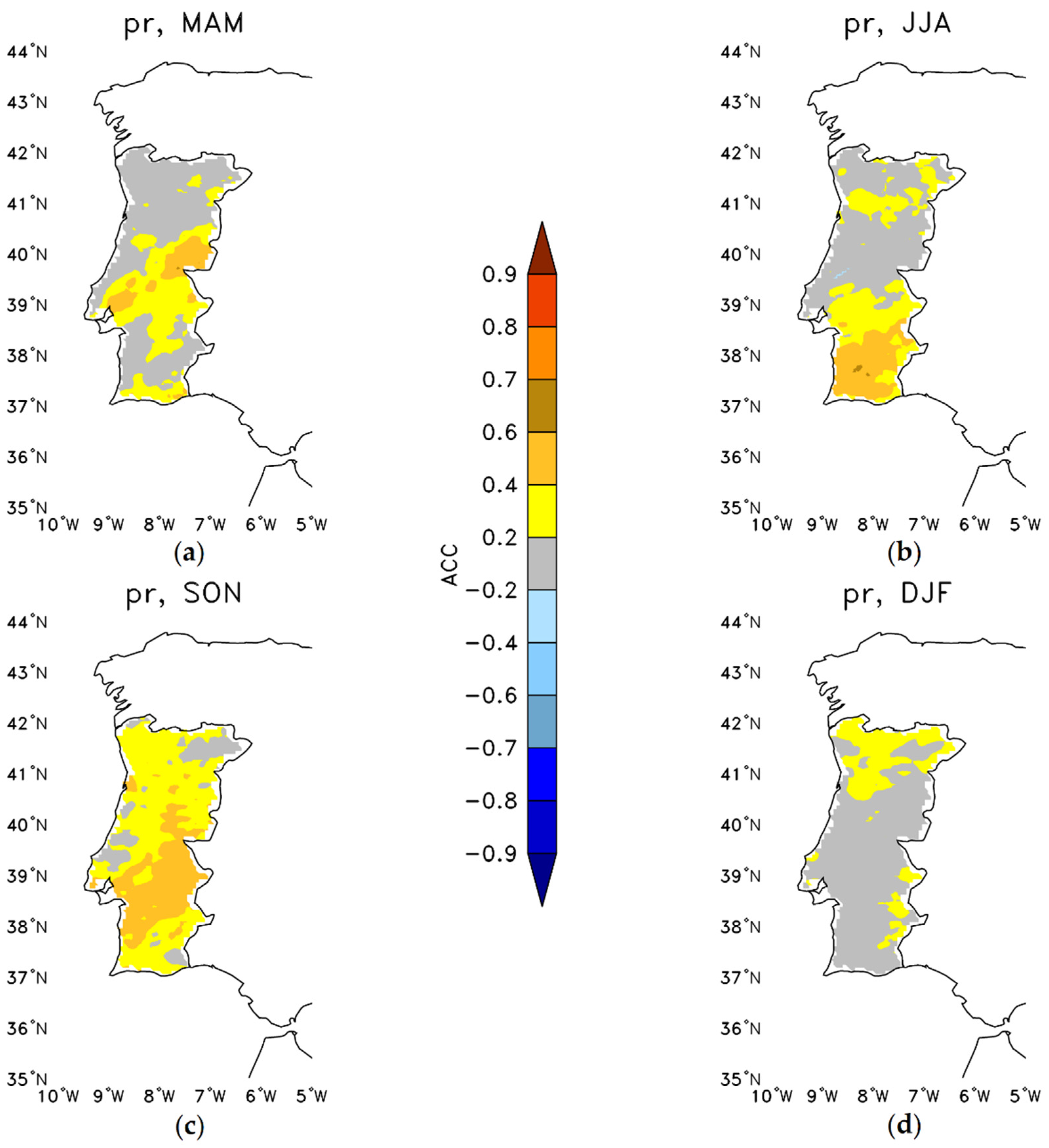
3.2.2. Precipitation

For precipitation, we analysed the relative deviations from its climatological mean (1995–2017). Again, we first looked at the global model output in Figure 7. For our regions under consideration, we find mostly small dry biases over Austria throughout the year. High values of precipitation bias appear over Germany in spring and in winter (Figure 7b,h). In some parts of central Germany wet biases exceed 100% in those two seasons.

In Portugal instead, the precipitation biases are smaller, with changing signs in summer/fall (Figure 7d,f)—dry—and winter/spring (Figure 7h,b)—wet. In winter season, the wet bias exceeds 60% in parts of the north of Portugal.

The precipitation bias of the downscaled seasonal hindcasts over Germany/Austria is shown in Figure 10. On the yearly average (Figure 10e), the bias is mostly below 10%, only small areas with wet biases from 10–20% appear. In spring (Figure 10a), we recognise a wet bias throughout a large part of the area, while in summer (Figure 10b) there tend to be dry biases over the western part of Germany. The Alpine region is well represented with only small wet biases in spring and fall (Figure 10a,c). The findings are in accordance with the results from Kreienkamp et al. [19], who found similar annual mean biases of downscaled historical GCM runs compared to HYRAS gridded observations [31] over Germany. Especially the large wet biases of the global model over Germany (spring and winter) could be considerably reduced and the dry bias over Austria has almost disappeared due to the statistical downscaling.

In the Portuguese study region, we find again wet biases of 10–20% on the annual mean in the downscaling results, which are located to the middle and north of the country (see Figure 11e). Unlike the German/Austrian case study region, the bias is more diversely distributed over the four seasons. While in spring (Figure 11a) the wet bias of the global model could be reduced and almost disappeared, in the summer season (Figure 11b) the signs alternate in the country. In fall (Figure 11c) there is a dry bias in the south which was already present in the global model. In winter (Figure 11d) a wet bias exceeding 40% is found throughout the country, which is not negligible. The global model also shows large precipitation biases for the Portuguese region for the winter season, which EPISODES does not seem to be able to correct completely.

4. Conclusions

We statistically downscaled seasonal climate forecasts for two hydrological case studies in the Clim2Power project. The global model, GCFS2.0, has limited skill of forecasting surface temperature and precipitation over Europe, which also applies for other seasonal prediction systems [11].

While there are general problems for precipitation, good hindcast skill of GCFS2.0 was found for temperature in southeastern Europe for the analysed initialisation months. Countries like Greece could profit from this. In the regions of our Clim2Power case studies in Germany/Austria and Portugal, the skill of both variables is quite low.

An improvement of hindcast skill can in some cases be achieved by using multi-model ensembles of seasonal forecasts, depending on season and region [38]. Beside this, an ensemble subsampling, based on a prediction of the NAO index can help to improve at least winter forecasts [12].

To generate spatially highly resolved data from the global model, we applied the empirical-statistical downscaling method EPISODES, a perfect prognosis method that is based on large-scale predictors for the variables of interest. The predictors of temperature and precipitation were determined by cross-validation to produce low-biased output for the considered region. Future studies could also include the hindcast skill in the selection of possible predictors to find an improved setup for the downscaling procedure.

In our study, no relevant increase or decrease of hindcast skill in terms of ACC due to downscaling could be detected for the two case study regions. In some parts of the countries, patterns slightly change compared to the global model, but still ACC values hardly exceed 0.5. In summary we find that the skill remains about the same, but the seasonal data is now available at a higher spatial resolution (approx. 6 km) which is the prerequisite for hydrological modelling.

Beside this we could show that the EPISODES method produces output with low biases, especially for temperature in Germany/Austria and Portugal throughout all seasons. On the annual average, the precipitation bias is mostly below 10% but with seasonal variations. Especially in winter, a wet bias remains for the Portuguese region.

Not only hydrologists can benefit from the high spatial resolution and the low bias of the seasonal data. In the Clim2Power project, also energy modelling and simulations of demand and concurrent water use were performed in the Portuguese case study. In order to support decision-making processes in the energy sector, it would be helpful to have more reliable seasonal forecasts. Nevertheless, it was possible to establish a modelling chain in the project, which can be used as soon as the seasonal forecasts gain skill.

For the future, an improvement in the prediction quality would be desirable. Possible starting points for this are on the one hand the improvement of the model itself (requires development), the increase of the number of ensemble members (requires more computing time), the use of multi-model seasonal forecasts (requires higher data volumes and transfer) or also the increase of the spatial resolution (requires also more computing time).

References

1. Gøtke, N.; Julkowska, D.; Serrano, J.; Ispas, I.; Amanatidou, E. Analysis of ERA-NET Cofund Actions under Horizon 2020; Final Report of the Expert Group; European Commission Publications: Luxembourg, 2016. [Google Scholar]
2. Simoes, S.G.; Amorim, F.; Frohlich, K.; Ostermoeller, J.; Saint-Drenan, Y.-M.; Assoumou, E.; Siggini, G.; Sessa, V.; Ranchin, T.; Gschwind, B.; et al. Clim2power—Translating climate data into power plants operational guidance. In Proceedings of the ICEE 2019—4th International Conference on Energy and Environment: Bringing together Engineering and Economics, Guimarães, Portugal, 16–17 May 2019; pp. 629–634. [Google Scholar]
3. Amorim, F.; Simoes, S.G.; Siggini, G.; Assoumou, E. Introducing climate variability in energy systems modelling. Energy 2020, 206, 118089. [Google Scholar] [CrossRef]
4. Simoes, S.; Nijs, W.; Ruiz, P.; Sgobbi, A.; Thiel, C. Comparing policy routes for low-carbon power technology deployment in EU—An energy system analysis. Energy Policy 2017, 101, 353–365. [Google Scholar] [CrossRef]
5. Kling, H.; Stanzel, P.; Fuchs, M.; Nachtnebel, H.-P. Performance of the COSERO precipitation–runoff model under non-stationary conditions in basins with different climates. Hydrol. Sci. J. 2015, 60, 1374–1393. [Google Scholar] [CrossRef]
6. Beça, P.; Simoes, S.G.; Mujtaba, B.; Diogo, P.; Amorim, F.; Carvalho, S.; Paes, P. CLIM2POWER Project: Seasonal forecasting for hydropower capacity in the Douro river basin—Portuguese case study. In Proceedings of the ECCA—European Climate Change Adaptation Conference, Lisbon, Portugal, 28–31 May 2019. [Google Scholar]
7. Bollmeyer, C.; Keller, J.D.; Ohlwein, C.; Wahl, S.; Crewell, S.; Friederichs, P.; Hense, A.; Keune, J.; Kneifel, S.; Pscheidt, I.; et al. Towards a high-resolution regional reanalysis for the European CORDEX domain. Q. J. R. Meteorol. Soc. 2015, 141, 1–15. [Google Scholar] [CrossRef]
8. MacLachlan, C.; Arribas, A.; Peterson, K.A.; Maidens, A.; Fereday, D.; Scaife, A.A.; Gordon, M.; Vellinga, M.; Williams, A.; Comer, R.E.; et al. Global Seasonal forecast system version 5 (GloSea5): A high-resolution seasonal forecast system. Q. J. R. Meteorol. Soc. 2015, 141, 1072–1084. [Google Scholar] [CrossRef]
9. Batté, L.; Déqué, M. Randomly correcting model errors in the ARPEGE-Climate v6.1 component of CNRM-CM: Applications for seasonal forecasts. Geosci. Model Dev. 2016, 9, 2055–2076. [Google Scholar] [CrossRef] [Green Version]
10. Johnson, S.J.; Stockdale, T.N.; Ferranti, L.; Balmaseda, M.A.; Molteni, F.; Magnusson, L.; Tietsche, S.; Decremer, D.; Weisheimer, A.; Balsamo, G.; et al. SEAS5: The new ECMWF seasonal forecast system. Geosci. Model Dev. 2019, 12, 1087–1117. [Google Scholar] [CrossRef] [Green Version]
11. Scaife, A.A.; Arribas, A.; Blockley, E.; Brookshaw, A.; Clark, R.T.; Dunstone, N.; Eade, R.; Fereday, D.; Folland, C.K.; Gordon, M.; et al. Skillful long-range prediction of European and North American winters. Geophys. Res. Lett. 2014, 41, 2514–2519. [Google Scholar] [CrossRef] [Green Version]
12. Dobrynin, M.; Domeisen, D.I.V.; Müller, W.A.; Bell, L.; Brune, S.; Bunzel, F.; Düsterhus, A.; Fröhlich, K.; Pohlmann, H.; Baehr, J. Improved Teleconnection-Based Dynamical Seasonal Predictions of Boreal Winter. Geophys. Res. Lett. 2018, 45, 3605–3614. [Google Scholar] [CrossRef] [Green Version]
13. Fröhlich, K.; Dobrynin, M.; Isensee, K.; Gessner, C.; Paxian, A.; Pohlmann, H.; Haak, H.; Brune, S.; Früh, B.; Baehr, J. The German Climate Forecast System: GCFS. J. Adv. Model. Earth Syst. 2021, 13, e2020MS002101. [Google Scholar] [CrossRef]
14. Feldmann, H.; Pinto, J.G.; Laube, N.; Uhlig, M.; Moemken, J.; Pasternack, A.; Früh, B.; Pohlmann, H.; Kottmeier, C. Skill and added value of the MiKlip regional decadal prediction system for temperature over Europe. Tellus A Dyn. Meteorol. Oceanogr. 2019, 71, 1618678. [Google Scholar] [CrossRef] [Green Version]
15. Reyers, M.; Pinto, J.G.; Moemken, J. Statistical–dynamical downscaling for wind energy potentials: Evaluation and applications to decadal hindcasts and climate change projections. Int. J. Climatol. 2015, 35, 229–244. [Google Scholar] [CrossRef] [Green Version]
16. Manzanas, R.; Lucero, A.; Weisheimer, A.; Gutiérrez, J.M. Can bias correction and statistical downscaling methods improve the skill of seasonal precipitation forecasts? Clim. Dyn. 2017, 50, 1161–1176. [Google Scholar] [CrossRef] [Green Version]
17. Manzanas, R.; Gutiérrez, J.M.; Fernández, J.; van Meijgaard, E.; Calmanti, S.; Magariño, M.E.; Cofiño, A.S.; Herrera, S. Dynamical and statistical downscaling of seasonal temperature forecasts in Europe: Added value for user applications. Clim. Serv. 2018, 9, 44–56. [Google Scholar] [CrossRef]
18. Taylor, K.E.; Stouffer, R.J.; Meehl, G.A. An Overview of CMIP5 and the Experiment Design. Bull. Am. Meteorol. Soc. 2012, 93, 485–498. [Google Scholar] [CrossRef] [Green Version]
19. Kreienkamp, F.; Paxian, A.; Früh, B.; Lorenz, P.; Matulla, C. Evaluation of the empirical–statistical downscaling method EPISODES. Clim. Dyn. 2018, 52, 991–1026. [Google Scholar] [CrossRef] [Green Version]
20. Eyring, V.; Bony, S.; Meehl, G.A.; Senior, C.A.; Stevens, B.; Stouffer, R.J.; Taylor, K.E. Overview of the Coupled Model Intercomparison Project Phase 6 (CMIP6) experimental design and organization. Geosci. Model Dev. 2016, 9, 1937–1958. [Google Scholar] [CrossRef] [Green Version]
21. Kreienkamp, F.; Lorenz, P.; Geiger, T. Statistically Downscaled CMIP6 Projections Show Stronger Warming for Germany. Atmosphere 2020, 11, 1245. [Google Scholar] [CrossRef]
22. Müller, W.A.; Jungclaus, J.H.; Mauritsen, T.; Baehr, J.; Bittner, M.; Budich, R.; Bunzel, F.; Esch, M.; Ghosh, R.; Haak, H.; et al. A Higher-resolution Version of the Max Planck Institute Earth System Model (MPI-ESM1.2-HR). J. Adv. Model. Earth Syst. 2018, 10, 1383–1413. [Google Scholar] [CrossRef]
23. Baehr, J.; Piontek, R. Ensemble initialization of the oceanic component of a coupled model through bred vectors at seasonal-to-interannual timescales. Geosci. Model Dev. 2014, 7, 453–461. [Google Scholar] [CrossRef] [Green Version]
24. Dee, D.P.; Uppala, S.M.; Simmons, A.J.; Berrisford, P.; Poli, P.; Kobayashi, S.; Andrae, U.; Balmaseda, M.A.; Balsamo, G.; Bauer, P.; et al. The ERA-Interim reanalysis: Configuration and performance of the data assimilation system. Q. J. R. Meteorol. Soc. 2011, 137, 553–597. [Google Scholar] [CrossRef]
25. Zuo, H.; Balmaseda, M.A.; Mogensen, K. The new eddy-permitting ORAP5 ocean reanalysis: Description, evaluation and uncertainties in climate signals. Clim. Dyn. 2017, 49, 791–811. [Google Scholar] [CrossRef]
26. Kalnay, E.; Kanamitsu, M.; Kistler, R.; Collins, W.; Deaven, D.; Gandin, L.; Iredell, M.; Saha, S.; White, G.; Woollen, J.; et al. The NCEP/NCAR 40-Year Reanalysis Project. Bull. Am. Meteorol. Soc. 1996, 77, 437–472. [Google Scholar] [CrossRef] [Green Version]
27. Kotlarski, S.; Szabó, P.; Herrera, S.; Räty, O.; Keuler, K.; Soares, P.M.; Cardoso, R.M.; Bosshard, T.; Pagé, C.; Boberg, F.; et al. Observational uncertainty and regional climate model evaluation: A pan-European perspective. Int. J. Climatol. 2019, 39, 3730–3749. [Google Scholar] [CrossRef] [Green Version]
28. Niermann, D.; Borsche, M.; Kaiser-Weiss, A.K.; Kaspar, F. Evaluating renewable-energy-relevant parameters of COSMO-REA6 by comparison with satellite data, station observations and other reanalyses. Meteorol. Z. 2019, 28, 347–360. [Google Scholar] [CrossRef]
29. Kaspar, F.; Niermann, D.; Borsche, M.; Fiedler, S.; Keller, J.; Potthast, R.; Rösch, T.; Spangehl, T.; Tinz, B. Regional atmospheric reanalysis activities at Deutscher Wetterdienst: Review of evaluation results and application examples with a focus on renewable energy. Adv. Sci. Res. 2020, 17, 115–128. [Google Scholar] [CrossRef]
30. Jacob, D.; Petersen, J.; Eggert, B.; Alias, A.; Christensen, O.B.; Bouwer, L.M.; Braun, A.; Colette, A.; Déqué, M.; Georgievski, G.; et al. EURO-CORDEX: New high-resolution climate change projections for European impact research. Reg. Environ. Chang. 2014, 14, 563–578. [Google Scholar] [CrossRef]
31. Rauthe, M.; Steiner, H.; Riediger, U.; Mazurkiewicz, A.; Gratzki, A. A Central European precipitation climatology ? Part I: Generation and validation of a high-resolution gridded daily data set (HYRAS). Meteorol. Z. 2013, 22, 235–256. [Google Scholar] [CrossRef]
32. Schulzweida, U. Climate Data Operators (CDO) User Guide; Zenodo: Meyrin, Switzerland, 2018. [Google Scholar]
33. Kottek, M.; Grieser, J.; Beck, C.; Rudolf, B.; Rubel, F. World Map of the Köppen-Geiger climate classification updated. Meteorol. Z. 2006, 15, 259–263. [Google Scholar] [CrossRef]
34. Illing, S.; Kadow, C.; Kunst, O.; Cubasch, U. MurCSS: A Tool for Standardized Evaluation of Decadal Hindcast Systems. J. Open Res. Softw. 2014, 2, e24. [Google Scholar] [CrossRef]
35. Kaiser-Weiss, A.K.; Borsche, M.; Niermann, D.; Kaspar, F.; Lussana, C.; Isotta, F.A.; van den Besselaar, E.; van der Schrier, G.; Undén, P. Added value of regional reanalyses for climatological applications. Environ. Res. Commun. 2019, 1. [Google Scholar] [CrossRef]
36. Lockhoff, M.; Zolina, O.; Simmer, C.; Schulz, J. Representation of Precipitation Characteristics and Extremes in Regional Reanalyses and Satellite- and Gauge-Based Estimates over Western and Central Europe. J. Hydrometeorol. 2019, 20, 1123–1145. [Google Scholar] [CrossRef]
37. Scherrer, S.C. Temperature monitoring in mountain regions using reanalyses: Lessons from the Alps. Environ. Res. Lett. 2020, 15, 044005. [Google Scholar] [CrossRef]
38. Mishra, N.; Prodhomme, C.; Guemas, V. Multi-model skill assessment of seasonal temperature and precipitation forecasts over Europe. Clim. Dyn. 2018, 52, 4207–4225. [Google Scholar] [CrossRef]
Figure 1. EPISODES model regions for Clim2Power’s case studies in Portugal and Germany/Austria. Crosses mark the regional grid points, which were used to determine the large-scale predictors.
Atmosphere 12 00304 g001
Figure 2. Anomaly Correlation Coefficient (ACC) of global GCFS2.0 data versus COSMO-REA6 (1995–2017). Both data sets were interpolated to a common grid (regular, 1°). The left column shows near-surface temperature (tas), the right column precipitation (pr). The rows display the meteorological boreal seasons spring (MAM) (a,b), summer (JJA) (c,d), fall (SON) (e,f) and winter (DJF) (g,h). Black dots represent significant correlation values (significance on 95% confidence level was determined by a bootstrap method using 500 bootstraps, [34]).
Atmosphere 12 00304 g002
Figure 3. Anomaly Correlation Coefficient (ACC) of near-surface temperature of GCFS2.0 hindcasts downscaled with EPISODES versus COSMO-REA6 (1995–2017) for the meteorological seasons (a) spring (MAM), (b) summer (JJA), (c) fall (SON), (d) winter (DJF).
Atmosphere 12 00304 g003
Figure 4. Anomaly Correlation Coefficient (ACC) of near-surface temperature of GCFS2.0 hindcasts downscaled with EPISODES versus COSMO-REA6 (1995–2017) for the meteorological seasons (a) spring (MAM), (b) summer (JJA), (c) fall (SON), (d) winter (DJF).
Atmosphere 12 00304 g004
Figure 5. Anomaly Correlation Coefficient (ACC) of precipitation of GCFS2.0 hindcasts downscaled with EPISODES versus COSMO-REA6 (1995–2017) for the meteorological seasons (a) spring (MAM), (b) summer (JJA), (c) fall (SON), (d) winter (DJF).
Atmosphere 12 00304 g005
Figure 6. Anomaly Correlation Coefficient (ACC) of precipitation of GCFS2.0 hindcasts downscaled with EPISODES versus COSMO-REA6 (1995–2017) for the meteorological seasons (a) spring (MAM), (b) summer (JJA), (c) fall (SON), (d) winter (DJF).
Atmosphere 12 00304 g006
Figure 7. Bias of the global GCFS2.0 hindcasts for near-surface temperature (left) and precipitation (right) compared to COSMO-REA6 (1995–2017) for the meteorological seasons spring (a,b), summer (c,d), fall (e,f) and winter (g,h).
Atmosphere 12 00304 g007
Figure 8. Bias of near-surface temperature from seasonal GCFS2.0 hindcasts downscaled with EPISODES vs. COSMO-REA6 (1995–2017) for the meteorological seasons (a) spring (MAM), (b) summer (JJA), (c) fall (SON), (d) winter (DJF) and (e) the annual mean.
Atmosphere 12 00304 g008
Figure 9. Bias of near-surface temperature from seasonal GCFS2.0 hindcasts downscaled with EPISODES vs. COSMO-REA6 (1995–2017) for the meteorological seasons (a) spring (MAM), (b) summer (JJA), (c) fall (SON), (d) winter (DJF) and (e) the annual mean.
Atmosphere 12 00304 g009
Figure 10. Bias of precipitation from seasonal GCFS2.0 hindcasts downscaled with EPISODES vs. COSMO-REA6 (1995–2017) for the meteorological seasons (a) spring (MAM), (b) summer (JJA), (c) fall (SON), (d) winter (DJF) and (e) the annual mean.
Atmosphere 12 00304 g010
Figure 11. Bias of precipitation from seasonal GCFS2.0 hindcasts downscaled with EPISODES vs. COSMO-REA6 (1995–2017) for the meteorological seasons (a) spring (MAM), (b) summer (JJA), (c) fall (SON), (d) winter (DJF) and (e) the annual mean.
Atmosphere 12 00304 g011