Abstract
Atmospheric gravity waves play a crucial role in affecting atmospheric circulation, energy transportation, thermal structure, and chemical composition. Using ERA5 temperature data, the present study investigates the tropospheric to the lower mesospheric gravity wave potential energy (EP) over the equatorial region to understand the vertical coupling of the atmosphere. EP is mainly controlled by two factors. The first is zonal wind through wave–mean flow interactions, and thus EP has periodic variations that are correlated to the zonal wind oscillations and enhances around the altitudes of zero-wind shears where the zonal wind reverses. The second is the convections caused by atmospheric circulations and warm oceans, resulting in longitudinal variability in EP. The lower stratospheric and the lower mesospheric EP are negatively correlated. However, warm oceanic conditions can break this wave energy coupling and further enhance the lower mesospheric EP.
1. Introduction
Atmospheric gravity waves (hereafter abbreviated as “gravity waves”) are mechanical oscillations of air parcels, which are generated by the force of gravity (as the restoring force) and an uplifting force such as buoyancy force [1,2]. Gravity waves can be excited by topography, convections, frontal systems, jet streams, wave–wave interactions, etc., as these sources can force air parcels upward [3,4,5]. They generate various kinds of gravity waves, e.g., mountain waves [6,7] and inertia–gravity waves [8,9], both of which are on the meso to synoptic scale. There are also Kelvin waves and (mixed) Rossby–gravity waves, which are equatorially trapped gravity waves on a planetary-scale [10,11].
Gravity waves transport energy and momentum from the lower to the middle and even the upper atmosphere, affecting the atmospheric circulations and energy budget [3]. They are related to several geophysical phenomena in the middle and upper atmosphere, such as the stratospheric quasi-biennial oscillation (QBO) [12,13,14], the upper stratospheric and lower mesospheric semiannual oscillations (SAO) [15,16,17], polar stratospheric clouds [18], sudden stratospheric warming events [19,20,21], elevated stratopause events [22,23], and mesospheric temperature inversions [24,25,26]. Further, the influences of gravity waves can also be seen in the ionosphere [1,27,28,29]. These waves are able to interact with atmospheric tides, which have a large contribution to the ionospheric morphology over the equatorial region [30,31,32].
Among these influences of gravity waves, the stratospheric QBO over the equatorial region is a very important quasi-periodic process due to its global effects on several geophysical and geochemical parameters and processes such as wind, temperature, meridional circulations, chemical processes, and even tropospheric weather and climate [12]. The stratospheric “zonal mean zonal wind” (abbreviated as “zonal wind” hereafter) over the equatorial latitudes is alternately westerly and easterly. It was believed that the westerly and easterly accelerations are mainly contributed by Kelvin waves and Rossby–gravity waves, respectively. However, recent studies show that a broad spectrum of non-planetary-scale gravity waves play a significant role to support the momentum balance and drive the QBO [10,12,13,33].
The stratospheric zonal wind QBO has periods varying from about 2 to 2.5 years. During the evolution of a QBO cycle, the westerly and easterly phases propagate downward as time goes by [12]. However, scientists observed that the westerly regime abnormally propagated upward in late 2015 and early 2016 [34,35]. This is the first anomalous event observed in the evolution of QBO. As the stratospheric QBO can affect the tropospheric weather and climate [12], the predictability of QBO is an important issue to weather and climate predictions [36]. Nevertheless, scientists did not foresee the 2015–2016 anomalous QBO, which reveals that our understanding regarding the dynamics of the QBO and atmospheric waves is still incomplete.
Gravity waves influence atmospheric wind and thermal structures [3,10,37], and therefore the wave activities can be observed either through the perturbations of wind, temperature, or pressure (e.g., [38,39,40]). Here we use the gravity wave potential energy, EP, which represents the temperature fluctuation caused by gravity waves. It needs only one vertical temperature profile to evaluate the EP value at a particular location and time (see details in Section 2.2; also refer to [41,42]). Nowadays, satellites and even reanalysis datasets can provide numerous temperature profiles worldwide, and therefore EP can be a good proxy to evaluate the activity of gravity waves. The global and seasonal distributions of EP have been studied using the temperature data from several satellite missions (e.g., [19,43,44,45,46,47,48,49,50,51,52]). Here we summarize some crucial facts regarding the stratospheric and lower mesospheric EP in the past literature, as mentioned above.
First, EP was found to be related to the zonal wind (mean flow) [43,47,48,49,50,51]. Both EP and the zonal wind have semiannual, annual, and quasi-biennial oscillations; also, the amplitude of each oscillation varies with altitude and latitude [43,47,48,49,50,51]. The semiannual signal is evident above the upper stratospheric (~40–45 km) altitude [49]. The tropical and mid-latitudinal EP experience maximum value during boreal winter months, especially in January and February [43]. Regarding the quasi-biennial variation in the stratosphere, EP is enhanced below the westerly shear of the zonal wind, which is defined as the zero zonal wind shear when the wind direction is changing from easterly to westerly [46,47,48,49,50].
Secondly, EP has latitudinal variations. Kelvin waves significantly contribute to the equatorial EP [45,47,50], whereas convections play an important role in the tropical EP [43,44,47,48,50,51]. The mid- and high-latitudinal EP are usually very low but may be high during winter months due to the influences of extratropical and polar systems [46,50,51].
Last, EP also has considerable longitudinal variations. The EP value is larger over continents than over oceans due to topographic effects, and larger over some areas with high convective activity over tropical latitudes [43]. Further, the spatial distribution of EP is controlled by synoptic weather systems and the interactions between weather systems and topography, as suggested by [51].
Most of these studies focused on only the stratospheric altitudes [19,43,44,45,46,47,48,50,51] except the one by [49], which has extended to the mesosphere and lower thermosphere. Besides, our previous paper [51] used 12-year temperature data from the Sounding of the Atmosphere using Broadband Emission Radiometry (SABER) instrument onboard the Thermosphere Ionosphere Mesosphere Energetics and Dynamics (TIMED) satellite. TIMED/SABER can be a good tool to study the long-term climatology of gravity wave activity, since it can provide vertical temperature profiles during the past ~19 years (December 2001–December 2020) [53]. However, there are two weaknesses of the TIMED/SABER data. First, SABER always directs to the anti-Sun side of the satellite resulting in asymmetric track-aligned, i.e., scattered distribution of the observations. Second, the instrument takes a 60-day period to cover all the 24-hr local time [53]. These two facts limit the usability of the SABER data, and the previous papers [49,50,51] usually took monthly or even seasonal mean results while using the data.
In the present study, we employed the temperature data retrieved from ERA5, which is the state-of-the-art reanalysis dataset provided by the European Centre for Medium-Range Weather Forecasts (ECMWF) (see detailed information in Section 2.1), to evaluate EP of atmospheric gravity waves. Compare with satellite data, reanalysis data are gridded data, and thus ERA5 can provide temperature profiles with much higher spatial and temporal resolutions. Hourly results are available using ERA5. Moreover, ERA5 provides data starting from 1979 (as of the writing of this paper). The double of the data period (compared with TIMED/SABER) enables us to study the gravity wave activities under different atmospheric and oceanic conditions with better accuracy. In addition, ERA5 contains the altitudinal range from the troposphere to the lower mesosphere. The upper mesosphere and lower thermosphere are covered by TIMED/SABER but not ERA5. Nevertheless, we believe that the ERA5 data can provide a better performance below the mesosphere while studying the spatio-temporal distribution of EP.
In our preceding paper [54], we had studied the morphology of wavenumbers 1 and 2 Kelvin waves in the equatorial stratosphere using ERA-Interim, which is the 4th (preceding) generation of the ECMWF’s reanalysis dataset. We have investigated the intra-QBO cycle and inter-QBO cycle variations, vertical distribution of wave amplitudes, and wave–mean flow interactions regarding Kelvin wave activities. Also, the correlations between convective indices and wave amplitudes were discussed. However, four questions still remain and need to be addressed: (1) we employed the space–time spectral method, two-dimensional fast Fourier transform (2D-FFT) [55], to obtain wave amplitudes. A 96-day segment was used to acquire wave amplitudes with a maximum wave period of 48 days, and therefore a temporal uncertainty of ±48 days (~1.5 months) exists in the output results; (2) longitudinal phase and variability were neglected and not discussed; (3) only the eastward propagated (Kelvin) waves were investigated, whereas the westward propagated waves are also important to explain the evolution of stratospheric QBO; (4) ERA-Interim only contains five model levels from 1.15 hPa to 0.1 hPa (~47–65 km altitude) in the mesosphere. Also, the investigation of mesospheric gravity waves is rare in the literature [49].
To address these questions in the present study, we will use another approach, EP of gravity waves, to investigate the wave activity over the equatorial region (±10° latitude). The equatorial gravity waves, especially the two kinds of planetary-scale waves of Kelvin wave and Rossby–gravity waves, are essential to maintain the alternation of the stratospheric zonal wind [12,33]. Studying the gravity wave activity in this area can help us understand the wave–mean flow interactions and further the evolution of the QBO [3], whereas the QBO plays an important role in global atmospheric dynamics and weather phenomena [12]. EP over the other latitudes is not included in this paper but shall be done elsewhere. The present work aims to study the spatio-temporal distributions of EP over the equatorial region and address the questions that are remaining from our preceding paper [54]. Also, the ERA5 dataset employed provides temperature data with a very high temporal resolution of 1 hour. We have a good opportunity to test the performance of ERA5 in estimating wave activities. Four objectives are set to be done in the present study: (1) detecting Rossby–gravity waves using EP; (2) constructing the climatology of EP from the troposphere to the lower mesosphere; (3) studying the longitudinal variation of EP; (4) finding the possible link between the ocean, the stratospheric EP, and the mesospheric EP. The results can provide us the most detailed equatorial gravity wave climatology, and will be quite useful information for us to understand the wave–mean flow interactions as well as the ocean–atmosphere coupling via gravity waves.
2. Data and Methods
2.1. ERA5 Reanalysis Data
ERA5 is the latest (5th generation) of the atmospheric reanalysis dataset released by ECMWF from 2017. The data period covers from 1979 to near real-time, and the ERA5 team is still working on the release of data from before 1979 [56,57]. In the present study, we used the temperature data during a 41-year period from 1979 to 2019. The data can be downloaded via the Copernicus Climate Data Store [58]. ERA5 is a four-dimensional variational (4D-Var) data assimilation using ECMWF’s Integrated Forecast System (IFS). Observations and measurements from land stations, radiosondes, dropsondes, aircraft, radars, satellites, etc., were assimilated to produce ERA5. The data cover the global atmosphere from the near-surface to 0.01 hPa (~80 km altitude) within 137 model levels defined by pressure. The vertical coordinate is converted from pressure model levels to altitudes according to the “L137 model level definitions” [59] in the present study. The horizontal resolution for ERA5 high resolution (HRES) data is about 31 km (0.28125°) in both latitude and longitude while the temporal resolution is one hour. The vertical resolution is not a fixed value. However, it varies with altitude, which is less than 0.4 km below 100 hPa (~16 km altitude, around the tropopause in the tropics) and ranging from 0.4 to 3 km between 100 and 1 hPa (~48 km altitude, around the stratopause). The detailed configuration, characteristics, and performance of ERA5 can be found in [57].
As the first attempt of using ERA5 data to study equatorial atmospheric waves, we decided to use a horizontal resolution of 2.5° in the present study as these waves are mostly planetary waves, and 2.5° resolution is sufficient to recognize them and their spatial variability. Since zonal wind plays an important role in interacting with waves and affecting the propagation of waves [3,10,12,13], we also retrieved zonal wind data from ERA5 for comparison.
2.2. Gravity Wave Potential Energy (EP)
The total energy density of gravity waves can be expressed as follows,
where and are the fluctuations of winds aligned and orthogonal to the direction of wave propagation, respectively. is the vertical velocity. is the observed temperature, while is the background (or mean) temperature. In the present study, is the vertical temperature profile retrieved from ERA5, and we employed a 2–10 km (the common vertical wavelengths of gravity waves in the stratosphere [3,60]) band-stop filter to filter out the wave components from , and the result is the background temperature . is the fluctuation term defined as . is the gravitational acceleration (–9.8 ms–2). is Brunt–Väisälä frequency defined as
where is the potential temperature and z is the altitude.
In Equation (1), the first three terms on the right-hand side represent the perturbations of waves acting on the background wind field and define the kinetic energy density of the gravity wave
Whereas, the last term in Equation (1) is the potential energy density of the wave, which corresponds to the temperature perturbations of waves in the form
Both theoretical predictions and observational results support a linear theory, in which the ratio of kinetic to potential energy is a constant [61,62]. Thus the gravity wave activity can be estimated using either EK or EP only. We chose EP to evaluate wave activity in the present study since it will be much easier to compare the results with recent studies. The variance term in Equation (4) is a function of and calculated as
where, and are the lower and upper altitudes over which the variance is calculated. Since we employed a 2–10 km filter to retrieve the wave component, the sliding window, i.e., the spacing between and is set to 2 km (the shortest wavelength) in the present study. While calculating the variance at altitude , and .
We noticed that the vertical wavelengths of mesospheric gravity waves are usually longer (up to 30 km) than stratospheric gravity waves [3]. However, it is technically impracticable to employ a 2–30 km band-stop filter to separate and from in Equations (1) and (4), because the scale (30 km) is almost equal to the mesospheric range (about 45–80 km altitude) as analyzed in the present study; also, the temperature inversion at the tropopause and stratopause will be wrongly recognized as wave structures. Therefore, a 2–10 km band-stop filter was employed, as mentioned in the earlier paragraph. Thereby, the mesospheric EP is possibly underestimated in the present study.
2.3. Data Preprocessing and EP Calculation
The ERA5 temperature data we downloaded are four-dimensional (longitude, latitude, altitude, and time) profiles at 137 model levels over the equatorial region of ±10° latitudes. The numbers of the longitudinal and latitudinal grids are 144 and 9, respectively, since the horizontal resolution is set to 2.5°. The calculation of EP requires data with equal spacing in altitude (Equation (5)). A linear interpolation of 0.2 km was performed to archived profiles with a fixed grid size from 0.2 to 80 km altitude. The hourly EP values over the equatorial region during the 41-year period from 1979 to 2019 were thus calculated. Also, the EP values below 5 km altitude and above 75 km altitude are unreliable because of the filtering process. We abandoned the values at these altitudes.
In the present study, we investigate the spatio-temporal distributions of equatorial EP, including the longitudinal, altitudinal, and temporal variations. Latitudinal information is not important since we only focus on a narrow latitudinal range of ±10°. Therefore, the EP values at the nine latitudinal grids were averaged, and a three-dimensional EP matrix containing the information on longitude, altitude, and time was created. Taking into consideration that the variations in the three dimensions are quite difficult to represent at the same time, in the following sections, we will present snapshots along a given dimension and/or calculate the mean values. The three-dimensional variations of EP will be concluded through the results and discussions on the two-dimensional ones.
3. The Longitude-Time Intensity of EP
We first check the performance of ERA5 in resolving wave activities. It has to be made sure that the two main kinds of planetary-scale gravity waves can be easily observed. The longitude-time intensity of EP (Figure 1) at a particular altitude can display the locations of high EP regions and the zonal propagating directions of the waves. This technique of conventional diagrammatic analysis has been widely used in many previous studies (e.g., [63,64,65,66,67]), to analyze the properties of planetary-scale waves with 1-day temporal resolution. The present study is the first one that attempts to perform this kind of analysis with 1-hour resolution.
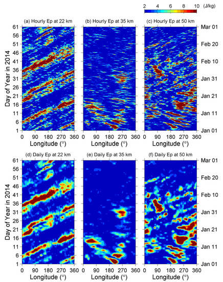
Figure 1.
(a–c) The hourly gravity wave potential energy, EP, and (d–f) the daily mean EP at 22, 35, and 50 km altitude, respectively, during the period from 1 January to 1 March 2014.
Since we have used a 41-year period of data that will be too long to show all the information using a longitude-time plot, we only show an example here. Figure 1a–c show the plots of hourly longitude-time intensity at 22, 35, and 50 km altitude, respectively, from 1 January to 1 March 2014. The plot at 22 km altitude (Figure 1a) shows some high EP regions that migrated eastward as time elapsed. These stripy structures are identified as Kelvin waves since their eastward-propagating pattern fits with the characteristics of Kelvin waves [10,11,63,64,65,66]. By tracking a particular target of the high EP region, the wave period can be determined. The wave period of those waves in Figure 1a was about 13–15 days, which is categorized as slow Kelvin waves [63].
On the other hand, Figure 1b plots some westward-propagating structures at 35 km altitude, which are considered to be caused by Rossby–gravity waves [10,65], and the wave period was about 2–5 days. At 50 km altitude in Figure 1c, the EP patterns are quite complex, implying that different kinds of waves were superposed here during this period. The waves seem to predominantly propagate westward in early January but eastward after mid-January.
Rossby–gravity waves have shorter wave periods (typically 4–5 days) and larger zonal wavenumbers (typically 4) compared to those of Kelvin waves [10,65]. Therefore, Rossby–gravity waves only leave trace evidence in the longitude-time plot (Figure 1b). As already mentioned, satellite data are scattered data with a revisit period of several to tens of days, and usually, a temporal resolution of 1 day is chosen to analyze those data (e.g., [63,64,65,66,67]). It is difficult to resolve the Rossby–gravity components using conventional satellite datasets without the use of space–time spectral analysis (e.g., [65]). To confirm this point, we plotted the daily EP, which is the daily mean of the hourly EP, in Figure 1d–f to demonstrate how the EP plots look if we used daily data instead of hourly data. The eastward-propagating structures of Kelvin waves are still seen using daily data in Figure 1d. However, most of the westward-propagating structures of Rossby–gravity waves become absent while using daily data in Figure 1e. Taking another example in Figure 1f, both the eastward- and westward-propagating structures are more obscure than those in the hourly plot of Figure 1c. Overall, the hourly results in Figure 1a–c, in which the EP values were evaluated using ERA5 data, are able to observe the equatorial gravity waves as we require. Moreover, the hourly data provided by ERA5 enable us to study wave activities on a shorter temporal scale than has ever been done before.
4. The Time-Altitude Intensity of EP
In this section, we report the EP distribution variability with time and altitude, i.e., the time-altitude intensity of EP. The values in the zonal direction are averaged and shown in Figure 2. The contour lines of zero zonal wind are also plotted to show the wave–mean flow interactions that affect the wave amplitudes [3,10,12,13]. The westerly shears of zonal wind are plotted using white contours without shadowing, while the white contours with magenta shadowing indicate the easterly shears of zonal wind. The figure can also be plotted using TIMED/SABER data. We have made a comparison between the ERA5 EP and TIMED/SABER EP in Supplementary Materials (Figures S1–S3 from the Supplementary Material).
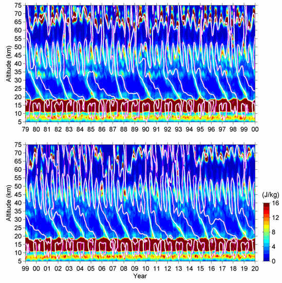
Figure 2.
The zonal mean EP in 1979–1999 (top) and 1999–2019 (bottom). The zero-wind shears of the zonal mean zonal wind are also overlaid on the plots. White contours indicate westerly shears, where the zonal wind reverses from easterly to westerly, and the white contours with magenta shadowing indicate easterly shears.
The features of the time-altitude intensity, as shown in Figure 2, can be divided into four regions: the troposphere, lower stratosphere, upper stratosphere, and lower mesosphere. We discuss the results from the lower to the higher altitudes one by one.
First, in the troposphere, EP peaks at 5–10 km altitude and around the tropopause. The former is plausibly related to meteorological systems such as convections since it appears in the middle troposphere and high EP values reflect the temperature disturbances caused by those systems. EP reaches an extreme value around the tropopause, where the temperature gradient varies sharply. This sharp change is extracted during the filtering process, resulting in a large difference between and , i.e., a large . Thus, the temperature variance here is not only contributed by wave activity but also by the filtering process [43].
Secondly, we look at 20–35 km altitude in the lower stratosphere. High EP regions are mainly distributed near and below the westerly shear. The EP values around the easterly shears are also slightly higher than the quiet background although this feature is not apparent in the figure. In contrast, the EP values during the westerly and easterly regimes (where and when the westerly/easterly wind prevails) are much lower than those around the zero-wind shears. EP in the lower stratosphere is significantly correlated with the zonal wind, which implies the existence of wave–mean flow interactions. We can further speculate that the high EP around the westerly and easterly shears could be mainly caused by Kelvin waves and Rossby–gravity waves, respectively, since both waves have significant contributions in driving the QBO of zonal wind [12]. We noticed that the EP contributed by Rossby–gravity waves is much smaller than Kelvin waves. This discrepancy comes from the differences between the amplitudes of Rossby–gravity waves ( is about 1 K in the lower stratosphere) and Kelvin waves ( is about 2–3 K) [10]. Besides, the wave activity tends to enhance from the late 1990s. The probable reason for this enhancement is the warming of sea surface temperature (SST), as reported in [54].
Thirdly, at the upper stratospheric altitude of 35–50 km, EP is high during the easterly phases of the upper stratospheric SAO (SSAO). In our preceding paper [54], we found that fast E1 (eastward wavenumber 1) Kelvin waves as well as some slow E1 Kelvin waves are not affected by the lower stratospheric zonal wind, and they can further propagate through the westerly regimes into the upper stratosphere. These waves amplify in the upper stratosphere below the westerly shears. It can also be seen that EP values show variability between different easterly phases of the SSAO.
Lastly, between 50 and 60 km altitude in the lower mesosphere, EP is very low, where the westerlies prevail most all the time. However, between 60 and 75 km altitude, EP becomes very large around but mainly above the zero-wind shears, where the zonal winds are easterly. We noticed a large difference in EP between the years before and after 2000. EP values are larger in the former period (the top panel of Figure 2) than in the latter period (the bottom panel of Figure 2). We suppose that this is not a real climatic change phenomenon since a large temperature bias in the lower mesosphere in the ERA5 dataset has been reported for the former period [68,69]. Also, the number of assimilated mesospheric data into ERA5 has a remarkable increase around 2001 (Table 14 in [56]), impacting the data reliability of mesospheric temperature. In spite of this, we retain the discussion on the mesospheric results for recognizing this problem regarding data stability and variability. The EP at 60–75 km altitude from late 2010 to 2014 is lower than that in other years. We also noticed that a La Niña event occurred in 2010–2012, and the Niño 3.4 index was mainly negative during the low EP period. The Niño 3.4 index is a specialized SST index used to monitor the evolution of El Niño/La Niña events. An El Niño/La Niña episode is defined when the 3-month smoothed Niño 3.4 index reaches the threshold of +/- 0.5 °C for several (usually five) consecutive months. Figure 3 shows the same EP values between 60 and 75 km altitudes along with the 3-month smoothed Niño 3.4 index issued by the Climate Prediction Center (CPC) of the National Oceanic and Atmospheric Administration (NOAA) [70]. It is seen that the EP values are larger during positive Niño 3.4 months than during negative Niño 3.4 months. In addition, the peak altitude of EP is higher during positive Niño 3.4 months and lower during negative Niño 3.4 months. A relationship between the Niño 3.4 index/El Niño events and Kelvin wave activities in the stratosphere has been studied by [71]. They found that Kelvin waves are enhanced during El Niño episodes. A special case during the 2009–2010 El Niño episodes has further accelerated the descent of the westerly phase of the stratospheric QBO. However, the correlation between the lower mesospheric EP and El Niño/La Niña events has not yet been studied before. We will continue the discussion on this aspect later in Section 6 and Section 7.3 using other approaches.
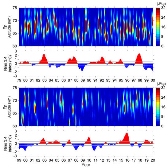
Figure 3.
The first and the third panels plot the zonal mean EP at 60–75 km altitude. The second and the fourth panels plot the Niño 3.4 index, and positive/negative values are stained with red/blue respectively. The two gray lines at ±0.5 °C indicate the thresholds of El Niño and La Niña events, respectively.
5. Cyclic Variations of EP
Equatorial wave activity highly correlates with the stratospheric QBO of zonal wind [3,10,12,13]. Nevertheless, the duration of a QBO cycle is not fixed. In our preceding paper [54], we attempted to convert the elapsed time (in days) to the phase of a QBO cycle and study the temporal and altitudinal variations of the Kelvin wave activity during different phases of a QBO cycle. The results are quite useful for us to understand the relationship between Kelvin waves and the QBO. In this section, we will employ the same method to study the cyclic variations of EP to understand the temporal and altitudinal evolution of the gravity wave activity.
The mean quasi-biennial, annual, and semiannual variations of EP will be discussed in this section. The quasi-biennial variation is correlated to the stratospheric QBO. We followed the definition in [54]. The beginning of a QBO cycle is defined as the day on which westerly shear descends to 20 km altitude, and the cycle ends when the next westerly shear descends to the same 20 km altitude. The semiannual variation is comprised of the SSAO and the lower mesospheric SAO (MSAO) which occurs between the stratosphere and the mesosphere. The MSAO in the present study does not indicate another SAO at 75–90 km altitude in the upper mesosphere but is a continuation of the SSAO. We chose the zonal wind at a 45 km altitude as a reference to further define the westerly phase and the easterly phase of the SAO. The 41-year time-averaged zonal wind is westerly from March to May and from September to November, and easterly from June to August and from December to February in the following year (as shown in Figure 5 later).
There are several other large-scale circulation systems (such as the Walker circulation) in the equatorial troposphere. Those systems can be modified by irregular variations (such as the southern oscillation and the Madden–Julian oscillation). Therefore, the zonal wind at the tropopause may be either westerly or easterly [10]. However, the zonal wind at the tropopause tends to be westerly during boreal winter and easterly during boreal summer. We define the annual oscillation (AO) of the zonal wind at a 14 km altitude, which is slightly lower than the tropopause (~16–18 km over the equator). The time-averaged zonal wind is westerly from November to May in the following year, and easterly from June to October (as shown in Figure 5 later).
5.1. Quasi-Biennial Variations
Figure 4 shows the 41-year time-averaged EP variation with QBO phase and altitude during a QBO cycle. The plots between –1 to 0 and 0 to 1 QBO cycle are exactly the same, and we repeat the plot since this will be easier to understand the temporal evolution of EP. Besides, the EP values above and below 20 km altitude are plotted separately with different color axis scaling since the EP values around the tropopause are very high.
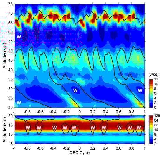
Figure 4.
The time-averaged zonal mean EP at 20–75 km (top; in linear color scaling) and 5–20 km (bottom; in logarithmic color scaling) altitudes. The elapsed time is standardized to the quasi-biennial oscillation (QBO) cycle (~29.4 months), and the –1–0 QBO cycle repeats the results in the 0–1 QBO cycle for a better illustration. The black contours plot the zero-wind shears of the time-averaged zonal wind, and the westerly regimes are marked.
There is no significant temporal variation below 20 km altitude, as seen in Figure 4, so we will focus on the altitudes above 20 km. As mentioned in Section 4, EP is evidently high around (but mainly a few km below) the westerly shears of the stratospheric QBO. In contrast, EP is also high but not apparent around the easterly shears.
The SSAO of the zonal wind is also seen in the figure. It implies a phase-lock relationship between the stratospheric QBO and SSAO, and so we can observe the SSAO structures in the figure based on the QBO phases. Both the QBO and the SSAO are considered to be partially driven by equatorial waves, and it is expected that the two oscillations are correlated. There are five SAO cycles during the period of a QBO cycle since the average duration of a QBO cycle is 29.4 months (calculated using the zonal wind data in 1979–2019). The westerly regime of the SSAO at –0.4/+0.6 QBO cycle (the fourth SSAO counting from the beginning of a QBO cycle) is found to connect with the westerly regime of the QBO because the zonal wind is easterly in the lower stratosphere. Kelvin waves can propagate to the upper stratosphere and further contribute a westerly acceleration to the zonal wind [12], resulting in the two westerly regimes connecting each other. In contrast to that, the westerly regime of the QBO is thickest at zero QBO cycle when the westerly shear reaches 20 km altitude. Most Kelvin waves cannot penetrate the thick westerly regime at this moment (as seen in Figure 3 and Figure 4, also referring to the results in [54]). With less acceleration from the lower stratosphere, the zero-wind shear of the SSAO at zero QBO cycle (the first SSAO in a QBO cycle) ascends to 47 km altitude. The effect is seen in the lower mesosphere too. The zero-wind shear of the MSAO descends to 64 km altitude at –0.05/+0.95 QBO cycle. Moreover, the westerly regime of this abnormal (first) SAO is the thinnest, and the thickness is only about a half compared to normal ones at 0.2 and 0.4 QBO cycles. The peak altitude of EP at 0.05 QBO cycle, which corresponded to the abnormal SAO in the lower mesosphere, is about 3–5 km lower than the normal ones.
5.2. Annual and Semiannual Variations
We will discuss annual variations together with semiannual variations since they have a common multiple of one year, and the related plots are shown in Figure 5. The 41-year EP values in each month from January to December were averaged individually to get the time-averaged EP in 12 individual months. The transverse axis in Figure 5 is defined as in the month of a year but not the SAO or AO phase since the former is more familiar.
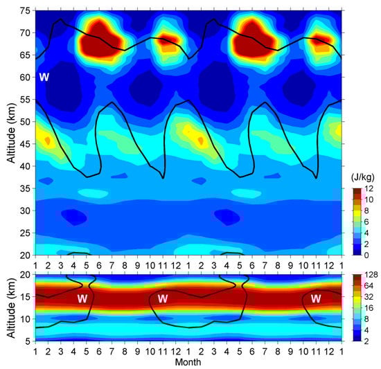
Figure 5.
Same as in Figure 4 but showing the zonal mean EP of each month.
Similar to Figure 4, there is no significant variation in mean EP below 20 km altitude, except for the peak altitude that shows an annual variation because of the annual variation in tropopause altitude. This annual variation extends to 25 km, which leads to a higher EP during boreal winter months than during boreal summer months. The westerly regime of the tropospheric zonal wind is the thickest from March to May during a year, and the westerly regime even invades the lower stratosphere during the same period. It is seen that EP is lower around 20 km altitude, and a low EP region appears at 27–30 km altitude during this period.
In the upper stratosphere, EP is high below the zero-wind shears of the SSAO, coinciding with the result as seen in Figure 4. Furthermore, the EP values in the easterly regimes are higher in the first half of the year (actually, from late December to March) than in the second half of the year (from June to September). In other words, the EP values are higher during the easterly phase of the first SSAO than that of the second SSAO in a year.
In the lower mesosphere, EP is again enhanced around easterly shears. Different from the SSAO, the EP values around the easterly shear of the second MSAO (which corresponds to the second SSAO) are higher than that of the first MSAO in a year. The difference between the first and the second SAO (either SSAO or MSAO) implies annual variations exist in the stratosphere and the mesosphere, and their annual variations are out of phase.
6. The Longitude-Altitude Intensity of EP
Figure 6 shows the longitude-altitude intensity of EP. Similar to Figure 4 and Figure 5, the values above and below 20 km altitude are plotted separately. All the values during the 41-year period were averaged to plot this figure.
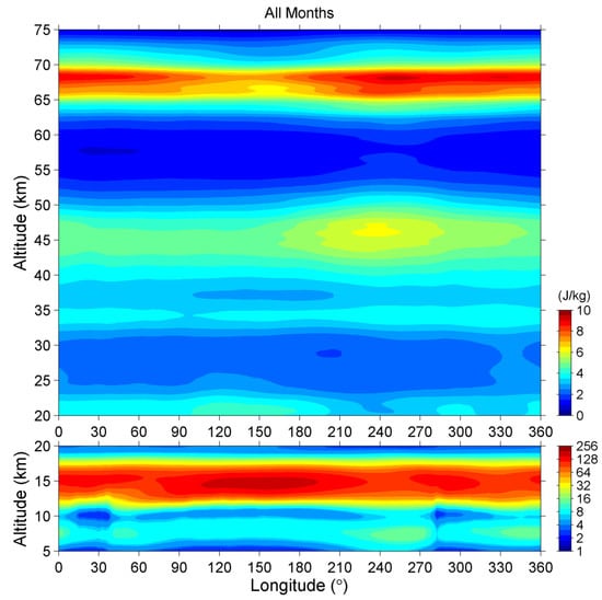
Figure 6.
The longitudinal variation of the full-time-averaged EP. The figure uses the same design for color scaling as Figure 4.
At ~7 km altitude in the lower troposphere, EP is higher around –50(310)–10°, 40–60°, and 210–280° longitudes. These sections correspond to the equatorial Atlantic Ocean, Western Indian Ocean, and Eastern Pacific Ocean, respectively. On the other hand, around the tropopause, EP is higher around –10(350)–60°, 110–190°, and 260–315° longitudes. These sections correspond to Africa, Maritime Continent (the islands and warm pools around Indonesia), and Southern America, respectively. The high EP regions in the lower troposphere and around the tropopause are complementary to each other. In other words, EP in the lower troposphere is higher around oceans, whereas EP around the tropopause is higher around continents and the Western Pacific warm pool. Overall, the highest EP value appears around the Maritime Continent, where the Walker circulation upwells under the non-El Niño condition. Similar to the result in Figure 5, the EP enhancements at the tropopause extend to the lower stratosphere, resulting in the longitudinal variability there. In the upper stratosphere and the lower mesosphere, the high EP regions center around 240° longitude, which is close to the upwelling of Walker circulation (around 210° longitude) in the troposphere under the El Niño condition.
We have found the possible dependence of EP on the Niño 3.4 index from Figure 3. The result further inspired us to calculate the mean EP values by separating the 41-year period into El Niño/La Niña months as well as westerly/easterly months of the SAO, QBO, and AO. Figure 7, Figure 8 and Figure 9 are the plots of longitude-altitude intensity under different conditions of SST/zonal wind at 5–20 km (Figure 7), 30–55 km (Figure 8), and 60–75 km (Figure 9) altitudes. In these figures, the all-month averaged EP, as shown in Figure 6, is repeated in each figure in panel (a). The results under different phases (westerly or easterly) of the SAO, QBO, and AO are plotted in panels (b–g), whereas, the results during El Niño and La Niña months are plotted in the last two panels of (h) and (i), respectively.
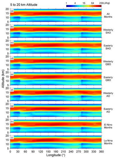
Figure 7.
The time-averaged EP at 5–20 km altitude under different conditions. (a) All months in the 41-year studying period; (b,c) westerly and easterly phases of the semiannual oscillation (SAO); (d,e) westerly and easterly phases of the quasi-biennial oscillation (QBO); (f,g) westerly and easterly phases of the annual oscillation (AO); (h,i) El Niño and La Niña episodes.
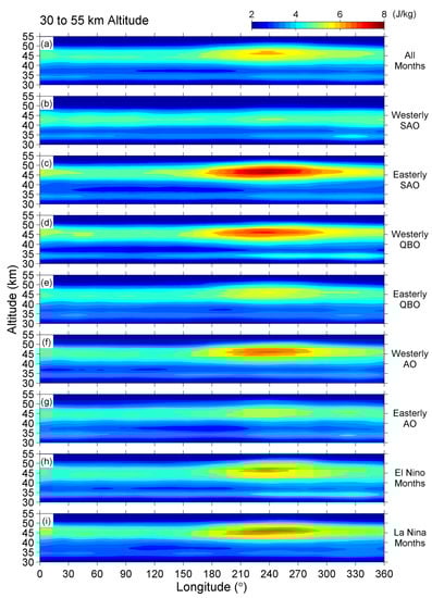
Figure 8.
Same as Figure 7, but showing the values at 30–55 km altitude with a different color axis scaling.
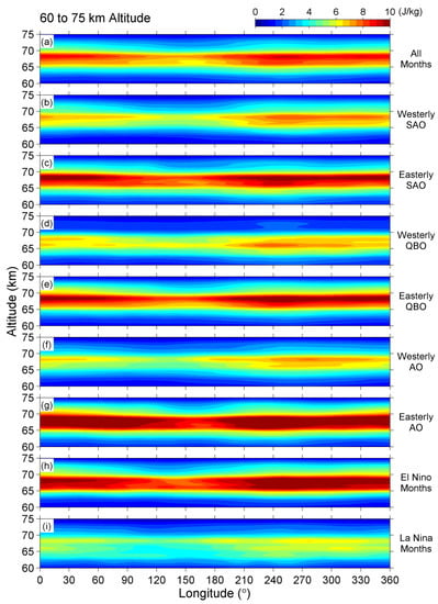
Figure 9.
Same as Figure 7 but showing the values at 60–75 km altitude with a different color axis scaling.
We first look at Figure 7. The EP values during the easterly phases of SAO and AO are slightly higher than those during the westerly phases. Also, the high EP region around the Maritime Continent extends westward during the easterly phases. However, there is no evident difference between the results of the easterly QBO and the westerly QBO. Although the EP values during El Niño and La Niña months are almost the same, the high EP region is located at 155–205° longitude during El Niño months, but it moves to 100–175° longitude during La Niña months, corresponding to the migration of the Pacific warm pool during El Niño and La Niña episodes.
As shown in Figure 2 and Figure 4, EP in the stratosphere is mainly contributed to by the high values below the westerly shears of the QBO caused by eastward-propagating waves, i.e., Kelvin waves. At a 45 km altitude in Figure 8, EP significantly varies with different phases of zonal wind oscillations. The phase of the QBO was defined as the zonal wind direction at 20 km altitude, as mentioned in Section 5. During the westerly phase of the QBO, the westerly regime becomes thinner as time elapses. Some Kelvin waves, which have a wavelength longer than the thickness of the westerly regime, are able to penetrate the westerly regime and further propagate to the upper stratosphere [54,72]. Those waves finally break around but below the westerly shears of the SSAO (also refer to Figure 4), resulting in higher EP during the westerly QBO and the easterly SAO (Figure 8c,d). Figure 8f,g show that EP is higher during the westerly phase than the easterly phase of the tropospheric AO, and the result is opposite to the tendency in the troposphere. Besides, Figure 8h,i reveal that EP at 45 km altitude is slightly higher under the La Niña condition.
EP at 60–75 km altitude is higher during the easterly phases of all the three zonal wind oscillations, as displayed in Figure 9. From the result of Figure 5, we know that the high EP regions in the lower mesosphere appear around the easterly shears, when and where the zonal wind reverses from westerly to easterly. Also, during the easterly QBO, the eastward-propagating Kelvin waves are not confined by the stratospheric zonal wind and are able to propagate upward. EP at 60–75 km altitude is thus higher during the easterly QBO. Figure 9f,g indicate that the annual variation of the lower mesospheric EP is in phase with the tropospheric EP. Both of them are higher during the easterly phase of tropospheric zonal wind. Figure 9h,i show that the lower mesospheric EP is higher under the El Niño condition than under the La Niña condition, which coincides with the result we found in Figure 3. Combining the results in Figure 6f–g and Figure 9f–i together, it seems there exists a link between the oceanic condition, the tropospheric EP, and the lower mesospheric EP. We will have more discussions on this topic in Section 7.3.
7. Discussions
7.1. Correlation Analysis of the Lower Stratospheric and the Lower Mesospheric EP
In Section 4 and Section 6, we have discussed the relationship between the Niño 3.4 SST index and the lower mesospheric EP, which indicates the ocean–lower mesosphere coupling. The coupling processes must have some effect in the intervening medium comprising of the troposphere and the stratosphere as the energy is transported upwards. The ocean–troposphere–stratosphere interactions regarding gravity wave activities have been investigated in earlier studies [51,54,71]. The same was also discussed using time-altitude and time-averaged intensity variabilities of EP in Section 4 and Section 5 of this paper, respectively. We extend the discussion to understand the correlation between the stratosphere and mesosphere.
The investigation is focused on the lower stratosphere and the lower mesosphere. The monthly EP values at the two altitudinal ranges of 20–35 km and 60–75 km were averaged to construct the time series of mean EP in the lower stratosphere and the lower mesosphere. These two time series are plotted in Figure 10a in light blue and light red, respectively. Since the lower mesospheric EP varied over a large range, the y-axis in Figure 10a is on a logarithmic scale.
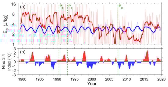
Figure 10.
(a) The light blue and light red curves plot the monthly zonal mean EP averaged in the lower stratosphere (at 20–35 km altitude) and lower mesosphere (60–75 km altitude). The bold blue and bold red curves plot the 12-month smoothed values of the light ones, i.e., the 12-month smoothed zonal mean EP, EP–12, in the lower stratosphere and lower mesosphere, respectively. (b) The Niño 3.4 index. The plot uses the same style as that in Figure 3. The dashed green lines indicate the three epochs that were tested using correlation analysis in Figure 11.
As already seen in Figure 4 and Figure 5, cyclic variations are the key features of the lower stratospheric and lower mesospheric EP. The two time series in Figure 10a, especially that of the lower mesosphere, also show these cyclic variations corresponding to semiannual, annual, and quasi-biennial periods. The semiannual and annual variations in EP are relatively regular since the corresponding oscillations in the background zonal wind are mainly triggered by solar radiation [10], and EP properly varies with the zonal wind (Figure 5). In contrast, the QBO of the stratospheric zonal wind is driven by upward-propagating waves formed in the lower atmosphere [12,13,71], and the oscillation has varied periods ranging from 23.8 to 34.4 months (during 1979–2014; the anomalous QBO in 2015–2016 [34,35] is not included). The variability in the QBO period can provide a good approach to examine the relationship between the EP value in the lower stratosphere and that in the lower mesosphere using correlation analysis. A 12-month moving average was applied to the two time series as mentioned earlier in the former paragraph (light curves in Figure 10a), to suppress the semiannual and annual signals in the time series. The results named the 12-month smoothed EP (EP–12), in the lower stratosphere (20–35km) and the lower mesosphere (60–75 km), are plotted in Figure 10a in bold blue and bold red, respectively. As seen in the figure, the variation in EP–12 in the lower stratosphere is quite regular, whereas the variation in the lower mesosphere is much more variable.
Previous studies [54,71] have demonstrated that the correlation analysis of stratospheric QBO needs to be made over a reasonable period with significantly fewer effects from other phenomena. If a very long period is examined, non-linear processes can play a crucial role in disturbing the relationship since correlation analysis is performed to examine the linearity of the two input parameters. In Section 4 and Section 6, we discussed that the lower mesospheric EP was significantly enhanced during El Niño episodes, i.e., when the Niño 3.4 index was positive (Figure 3 and Figure 9). However, the sensitivity of the lower stratospheric EP to the polarity of the Niño 3.4 index is much lower than that in the lower mesosphere. The upper stratospheric EP is also higher during La Niña than El Niño episodes (Figure 8).
The alternation of positive and negative Niño 3.4 index (or another SST index) is a natural phenomenon. It is not possible to find a long period when the oceanic and atmospheric environments are always uniform. Therefore, we chose a period when the variation of the Niño 3.4 index (repeated in Figure 10b) is relatively regular. Besides, as mentioned in Section 4, the lower mesospheric EP is significantly larger before than after 2000. We chose two epochs centered at mid-2007 (i.e., July 2007 or 2007.5, we use the latter one for a simplified expression though this is not a common usage; marked as Pa in Figure 10a) and mid-1990 (1990.5; Pb) which are before and after 2000, respectively, to perform the correlation analysis. As a contrast to these two “ideal” epochs, the same analysis was also applied to another “defective” epoch centered over January 1993 (1993.0; Pc). The Niño 3.4 index was mostly positive during the five-year period from 1990 to 1994.
We have tested different lengths of the examining period ranging from 1 to 10 years with 2-month stepping to obtain the correlation coefficient between EP–12 values in the lower stratosphere and lower mesosphere. Besides, for each examining period, the lag correlation was calculated by shifting the lower stratospheric EP–12 from –32 to 32 months to determine the occurrence of high (either positive or negative) correlation, which indicates the phase difference between the lower mesospheric and the lower stratospheric EP–12. The time shift was limited to ±32 months since the correlation pattern repeats every QBO cycle (as can be observed in Figure 11 later) and the average period of a QBO cycle was 29.4 months.
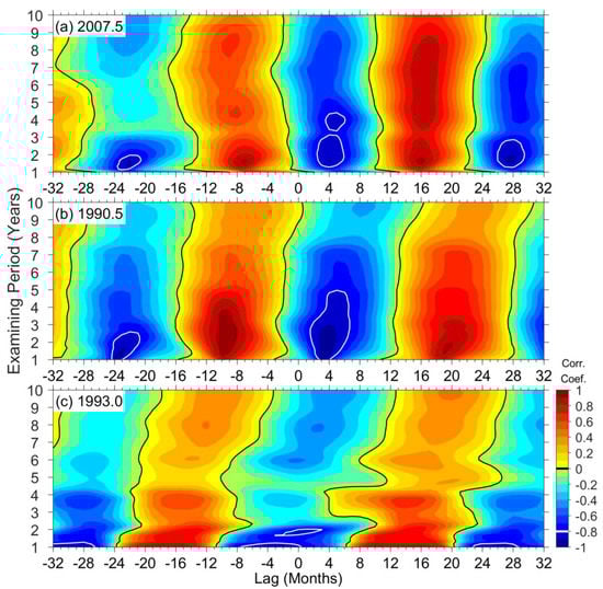
Figure 11.
The correlation coefficients between the lower stratospheric and lower mesospheric EP–12, as functions of lag time and examining period centered over three epochs of (a) 2007.5, (b) 1990.5, and (c) 1993.0, respectively.
Here we take an example of using a 1-year examining period centered at Pa (2007.5) to understand the analysis procedure better. The EP–12 values in the lower mesosphere (60–75 km altitude) from January to December 2007 were taken, while with 1 (–1) month shift time, the EP–12 values in the lower stratosphere (20–35 km altitude) from February 2007 to January 2008 (from December 2006 to November 2007) were taken during the calculation of the correlation coefficient. The process was repeated numerous times for –32 to 32-month shifts, and from 1 to 10-year examining periods (stepped in 2 months).
The analysis results are correlation coefficients as functions of the lag time (the additive inverse of shift time) and the examining period and are illustrated in Figure 11. Each plot in the figure corresponds to the results of one epoch as defined earlier. A positive lag indicates that the lower mesospheric EP–12 lags behind the lower stratospheric EP–12, whereas a negative lag indicates an opposite situation, in which the lower mesospheric EP–12 leads ahead.
We first check the common features in all three plots in Figure 11. The correlation pattern repeats every 24–30 months. The recurrence period was about 24 months for Pa (Figure 11a) but about 30 months for Pb (Figure 11b), as the period of stratospheric QBO around Pa (2007.5) was shorter than that around Pb (1990.5) (Figure 2). Besides, the correlation becomes lower while taking a longer examining period, and this fits in with our earlier expectation and also the conclusions of the previous study [71].
7.2. Analysis Results and the Correlationship between the Lower Stratospheric and Lower Mesospheric EP–12
For the two ideal cases (Pa and Pb; Figure 11a,b) with a short examining period (≤5 years), the negative correlations both peak at 4 months, whereas, the positive correlations peak at 16 and –7 months for Pa, and 20 and –9 months for Pb, respectively. The maximum magnitudes (taking absolute values here) of the correlation coefficient in both cases are larger than 0.9, indicating that the lower mesospheric EP–12 is highly (either positive or negative) correlated with the lower stratospheric EP–12 but with a time delay. The magnitude of positive correlation is slightly higher than that of negative correlation, though this discrepancy is very small and difficult to recognize from the figure, considering we are investigating the wave energy coupling by examining the correlation of two time series that both vary with the QBO cycle. The waves transport energy upward [12,13,71], and the variation of the mesospheric EP–12 must lag behind the lower stratospheric EP–12, i.e., positive lags present the cause-effect relationship and are geophysically important. In Figure 11a,b, there are two possibilities with positive lag time. One is the negative correlation with a 4-month lag, and the other one is the positive correlation with 16- and 20-month lags for Pa and Pb, respectively. The negative one has a much shorter lag time, whereas, the positive one has a slightly higher correlation. We have to consider these results carefully to properly interpret the wave energy coupling between the lower stratosphere and the lower mesosphere.
The drive of QBO is theoretically explained by the wave–mean flow interactions in the stratosphere [10,12,73]. Gravity waves propagate upward and are amplified with increasing altitude. When the waves meet the zonal wind with a flow velocity that is close to their phase velocity, the eastward-(westward-) propagating waves break around the westerly (easterly) shear, and produce a westerly (easterly) acceleration of the zonal wind. Both the zero-wind shears and the altitude where the waves break, named the “critical level”, will move downward as time progresses. Thus, waves drive the alternation of zonal wind direction, i.e., the zonal wind QBO (see literature [10,12,73] for a detailed explanation of the mechanisms of the stratospheric QBO). While waves break at the critical level in the lower stratosphere, the amplitude of the waves is amplified, and the wave energy observed here is significantly enhanced (see Figure 2 and Figure 4 for practical examples). However, at any time, some waves do not fit the wave breaking condition (i.e., do not meet their critical level). They are able to penetrate the zonal wind to reach higher altitudes. In general, considering the wave energy generated around the tropopause is a fixed value, the more the wave energy is dissipated or blocked in the lower atmosphere, the less it can propagate upward into the upper atmosphere. Therefore, EP–12 in the lower mesosphere shall be negatively correlated to that in the lower stratosphere.
Now we go back to the results of Figure 11a,b. Both the negative correlations for Pa and Pb have a 4-month lag. It means EP–12 in the lower mesosphere lags 4 months behind EP–12 in the lower stratosphere. The vertical group and phase velocities of gravity waves in the stratosphere and mesosphere have been investigated using radar observations [74,75] and model simulations [76]. Both the two velocities are usually on the scale of <1 to a few ms–1, though their vertical components are opposite. For a wave source in the troposphere, e.g., a deep convection system that excites gravity waves, the wave it generates can propagate upward through the stratosphere and further reach the mesosphere within several hours to a few tens of hours (considering a vertical group velocity of 1 ms–1), if the waves are not blocked by the background zonal wind. However, the wave–mean flow interactions drive the long-term variation (QBO) of the zonal wind in the lower stratosphere, and in the meanwhile, some waves are restrained in the stratosphere, but other waves are able to propagate and transport energy upward. In the mesosphere, those waves again partially interact with the zonal wind there and some are restrained, but the rest further propagate upward to a higher altitude. The wave energy budget in the mesosphere is composed of incoming, outgoing, and dissipating energies. Although the waves can reach the mesosphere quickly due to their “fast” phase and group velocities, from the climatological view, the wave energy budget (including the contribution and adjustment of wave–mean flow interactions in the lower mesosphere) takes about 4 months (Figure 11a,b) to attain a balance. Since the lower mesospheric EP–12 is negatively correlated to the lower stratospheric EP–12 with a 4-month lag, the long-term lower mesospheric EP shall experience its minimum value while 4 months after the maximum of the long-term lower stratospheric EP, with a prerequisite that the oceanic condition is normal (non-El Niño).
7.3. Modification of the Wave Energy Coupling under Warm Oceanic Conditions
In Figure 11c, we also show the result of the correlation analysis for Pc. As the example of a “defective” case, this epoch (1993.0) was centered around a 5-year period of positive Niño 3.4 index, i.e., the ocean was under warm conditions. The correlation pattern (Figure 11c) is quite different from those for Pa and Pb (Figure 11a,b), especially the bottom part of the plot. For a very short examining period, the negative correlation peaks around –4 months, i.e., the lower mesospheric EP–12 leads ahead the lower stratospheric EP–12, which is not reasonable as the waves originate in the lower atmosphere and propagate upward to the upper atmosphere. While the examining period increases, the influence from the warm oceanic period is diluted, and the lag of the negative correlation migrates to a positive value around 4 months, which is the same as the results of Pa and Pb, though the magnitude of the correlation coefficient becomes much lower.
Figure 10a shows that the lower mesospheric EP–12 maintained a high level during the positive Niño 3.4 period in 1990–1994 compared to other years before 2000. The warm oceanic condition favors the development of convections, and those convections can excite gravity waves that propagate upward into the upper atmosphere (see [3,11,71] and references therein). However, from Figure 10a, we also note that the amplitude of the lower stratospheric EP–12 is quite regular, always varies between 2 and 4 J/kg, and seems not to be affected by the oceanic condition. Although we cannot explain the mechanism of why the lower stratospheric EP–12 is limited to such a range at this moment, the result reveals that the stratosphere does not fully block the upward propagation of gravity waves, even though the gravity wave activity is expected to be very active during warm oceanic periods, such as the anomalous Niño 3.4 event in 1990–1994. In this situation, for those waves that are not restrained by the stratosphere, they are able to further propagate to the mesosphere, and their amplitude is amplified because of either the decrease in air density or wave breaking around the critical level in the mesosphere. Those processes result in the enhancements of EP during El Niño episodes and positive Niño 3.4 anomalies, as observed in Figure 3, Figure 9 and Figure 10. In addition, the enhanced gravity waves may propagate further into the thermosphere directly or indirectly via secondary wave generation, under favorable conditions, and influence both the neutral atmosphere and ionized particles, i.e., the ionosphere. Many papers have reported the correlation between the El Niño-Southern Oscillation (ENSO) and thermospheric tides, ionospheric E region scintillations, and total electron content (TEC) fluctuations (e.g., [77,78,79,80]), indicating dynamic ocean–atmosphere coupling via gravity waves.
7.4. The Lower Mesospheric EP during the 2015–2016 Anomalous QBO
It is also worth paying attention to the period of the 2015–2016 anomalous QBO. In late 2015 and early 2016, the descending westerly regime showed upward propagation and interrupted the development of the downward easterly in the upper stratosphere. Meanwhile, another easterly regime developed inside the westerly regime in the lower stratosphere. The illustration of the QBO evolution during 2015–2016 is available in Figure 2, and diagnostic analyses of this anomalous QBO event have been done by [34,35]. This anomalous feature was attributed to the invasion of extratropical Rossby waves and subsequent breaking in the equatorial stratosphere in late 2015. The extreme El Niño event in 2015–2016 also played an important role in ushering the westward momentum into the equatorial stratosphere.
There was a 4-year period from 2010 to 2013 when the Niño 3.4 index mainly negatively deviated before the extreme El Niño event. We find here that the lower mesospheric EP was extremely low during this negative Niño 3.4 period. However, the lower mesospheric and the lower stratospheric EP–12 are still negatively correlated (Figure 10a). Later in 2015, as the Niño 3.4 index dramatically increased, the lower mesospheric EP–12 also quickly enhanced. Nevertheless, the lower mesospheric EP–12 is no longer negatively correlated with the lower stratospheric EP–12, as the latter also was enhanced due to the QBO variation. The periodic modulation of the stratosphere–mesosphere wave energy coupling was disrupted during the 2015–2016 extreme El Niño and anomalous QBO event. The effect remained for a long time, until the end of our EP–12 data in mid-2019, even though the oceanic condition returned to normal. We also found the westerly in the lower mesosphere was abnormally strong during the period of EP enhancement. The westerly at 55–65 km altitude is routinely interrupted by easterly every 3–5 MSAO cycles (Figure 2). The effect can be considered as the superposition of the easterly phase of the MSAO and mesospheric QBO. However, the westerly maintained 8 MSAO cycles in 2015–2018 before the zonal wind reversed to easterly (Figure 2). Thus, the anomalous oceanic and atmospheric conditions not only disturbed the stratospheric QBO but also produced a chain reaction affecting the lower mesospheric zonal wind and wave activity.
8. Summary and Conclusions
Studies regarding equatorial atmospheric gravity waves are crucial due to the influence of waves on the atmospheric circulations and energy budget [3]. We had investigated the morphology and climatology of equatorial Kelvin waves using the method of 2D-FFT in our preceding paper [54]. However, some questions remained and needed to be answered (see the last two paragraphs in Section 1). In the present study, we considered the temperature profiles provided by the ERA5 reanalysis data to evaluate gravity wave potential energy, EP, over the equatorial region (±10° latitude). ERA5 provides gridded temperature profiles at 5–75 km altitude during 1979–2019, enabling us to study the longitudinal and altitudinal morphology as well as the climatology of gravity wave activity. The main findings of this paper are summarized below.
- (1)
- EP is enhanced below the westerly shears and around the easterly shears of the stratospheric QBO, and the enhancements correspond to Kelvin waves and Rossby–gravity waves, respectively (Figure 2). EP is also high around the zero-wind shears below and above the westerly regime in the upper stratosphere and lower mesosphere (Figure 5). Wave activities can modify the thickness of this westerly SAO. While the westerly regime of the lower stratospheric QBO is the thickest at the beginning of a QBO cycle, most Kelvin waves are confined and not able to propagate upward, resulting in the decrease of westward acceleration in the upper stratosphere and lower mesosphere, and the thickness of the westerly SAO is thus reduced (Figure 4).
- (2)
- All the three peaks of EP values at 15 km, 45 km, and 65–70 km altitudes have longitudinal variability. The EP value at 15 km altitude peaks around the Maritime Continent, where the Walker circulation upwells under the non-El Niño condition. The EP at 45 km and 65–70 km peaks around 240° longitude, which is close to the upwelling of Walker circulation under El Niño condition (Figure 6).
- (3)
- The highest EP around the tropopause migrates with the Pacific warm pool, located at 155–205° longitude during El Niño months but 100–175° longitude during La Niña months (Figure 7). The stratospheric EP is higher during the westerly QBO and AO than the easterly QBO and AO. In contrast, the upper stratospheric EP is higher during the easterly SAO and La Niña months than the westerly SAO and El Niño months (Figure 8). In the lower mesosphere, EP is higher during the easterly phases than the westerly phases of all the three zonal wind oscillations (Figure 9).
- (4)
- The stratospheric zonal wind dominates the upward propagation of gravity waves (Figure 2 and Figure 4). Waves are either restrained in the stratosphere or able to propagate into the mesosphere further. The long-term (12-month smoothed) lower mesospheric EP is highly negatively correlated with the lower stratospheric EP. The former lags 4 months behind the latter while leaving their annual and semiannual variations aside (Figure 11). However, waves are very active under warm oceanic conditions, and the upward-propagating wave energy can exceed the limitation that the stratosphere can adjust to. The lower mesospheric EP is thus significantly enhanced during El Niño episodes.
- (5)
- During the 2015–2016 extreme El Niño and anomalous QBO event, not only the lower mesospheric EP was enhanced, but also the westerly was more strengthened than usual there.
This paper investigates the spatio-temporal distributions of EP over the equatorial region and finds the possible link between the oceanic condition and gravity wave activities. On the basis of the results mentioned above, we can conclude that the gravity wave EP is greatly affected by zonal winds via the wave–mean flow interactions. EP usually enhances near the zero-wind shears, indicating that the wave activity is also high there. The oceanic condition is another essential controlling factor that affects the wave activity and EP. The warm oceanic condition favors convections, and it is able to excite gravity waves. Once the wave energy restrained by the zonal wind in the stratosphere is “saturated”, the waves can propagate upward into the lower mesosphere, intensifying the EP value there. This ocean–stratosphere–mesosphere coupling is very important to explain the enhancement of mesospheric wave activity during El Niño episodes. Its effect may further propagate into the ionosphere modifying the ionospheric morphology (e.g., [77,78,79,80]).
Gravity waves affect the middle atmospheric dynamics, and their effects may further influence the atmosphere on a global scale [3]. The present study can help us to understand the normal state (climatology) of the gravity wave activity in the equatorial troposphere, stratosphere, and lower mesosphere. Also, the wave energy coupling between the ocean and the mesosphere is revealed. Based on the knowledge of gravity wave climatology, continuous monitoring of the equatorial EP may be useful for us to diagnose anomalous events regarding the gravity wave activity in the past (e.g., the 2010 fast descending of westerly QBO [71] and the 2015–2016 anomalous QBO [34,35]) and in the future.
Supplementary Materials
The following are available online at https://www.mdpi.com/2073-4433/12/3/311/s1, Supplementary material S1. A Comparison Between EP Obtained from ERA5 and TIMED/SABER. Supplementary material S2. Remarks on the ERA5 and SABER Temperature Data and Their Application on Evaluating EP [81,82,83,84,85,86,87]. Figure S1: The zonal mean EP in (a) 1999–2019 obtained from ERA5 and (b) 2002–2019 obtained from the Thermosphere Ionosphere Mesosphere Energetics and Dynamics/ Sounding of the Atmosphere using Broadband Emission Radiometry instrument (TIMED/SABER). Figure S2: Same as Figure S1, but showing normalized EP. Figure S3: The typical profiles of (a) temperature, (b) background temperature, (c) temperature fluctuation, (d) square term of Brunt-Väisälä frequency, and (e) potential energy, as observed by SABER.
Author Contributions
Conceptualization, S.-S.Y. and C.-J.P.; Data curation, S.-S.Y.; Formal analysis, S.-S.Y.; Funding acquisition, C.-J.P.; Investigation, S.-S.Y.; Methodology, S.-S.Y., C.-J.P., and U.D.; Project administration, C.-J.P.; Supervision, C.-J.P.; Validation, C.-J.P. and U.D.; Writing—original draft, S.-S.Y.; Writing—review & editing, C.-J.P. and U.D. All authors have read and agreed to the published version of the manuscript.
Funding
Shih-Sian Yang and Chen-Jeih Pan are supported by the Ministry of Science and Technology of Taiwan through the grants MOST–109–2811–M–008–542 and MOST–109–2111–M–008–003. Uma Das is supported by the Science and Engineering Research Board (SERB), a statutory body of the Department of Science and Technology (DST), Government of India, through the Early Career Research Award (ECRA) grant ECR/2017/002258.
Institutional Review Board Statement
Not applicable.
Informed Consent Statement
Not applicable.
Data Availability Statement
The ERA5 data is processed and carried out by ECMWF within the Copernicus Climate Change Service (C3S), and the data can be retrieved from https://cds.climate.copernicus.eu/ (accessed on 27 February 2021). The Niño 3.4 index was provided by the Climate Prediction Center (CPC) of the National Oceanic and Atmospheric Administration (NOAA) and can be downloaded at https://origin.cpc.ncep.noaa.gov/products/analysis_monitoring/ensostuff/ONI_v5.php (accessed on 27 February 2021).
Acknowledgments
The authors thank five anonymous reviewers for their helpful comments and suggestions on this paper. The authors acknowledge the Copernicus Climate Change Service (C3S), which is operated by European Centre for Medium-Range Weather Forecasts (ECMWF), and National Oceanic and Atmospheric Administration (NOAA) for opening the data access.
Conflicts of Interest
The authors declare no conflict of interest.
References
- Hines, C.O. Internal Atmospheric Gravity Waves at Ionospheric Heights. Can. J. Phys. 1960, 38, 1441–1481. [Google Scholar] [CrossRef]
- Nappo, C.J. An Introduction to Atmospheric Gravity Waves; Academic Press: Amsterdam, The Netherlands, 2012; Volume 102. [Google Scholar]
- Fritts, D.C.; Alexander, M.J. Gravity wave dynamics and effects in the middle atmosphere. Rev. Geophys. 2003, 41, 1003. [Google Scholar] [CrossRef]
- Fritts, D.C.; Nastrom, G.D. Sources of mesoscale variability of gravity waves. Part II: Frontal, convective, and jet stream excitation. J. Atmos. Sci. 1992, 49, 111–127. [Google Scholar] [CrossRef]
- Nastrom, G.D.; Fritts, D.C. Sources of mesoscale variability of gravity waves. Part I: Topographic excitation. J. Atmos. Sci. 1992, 49, 101–110. [Google Scholar] [CrossRef]
- Durran, D.R. Mountain waves and downslope winds. In Atmospheric Processes over Complex Terrain; Blumen, W., Ed.; American Meteorological Society: Boston, MA, USA, 1990; pp. 59–81. [Google Scholar] [CrossRef]
- Eckermann, S.D.; Preusse, P. Global measurements of stratospheric mountain waves from space. Science 1999, 286, 1534–1537. [Google Scholar] [CrossRef] [PubMed]
- Tsuda, T.; Murayama, Y.; Wiryosumarto, H.; Harijono, S.W.B.; Kato, S. Radiosonde observations of equatorial atmosphere dynamics over indonesia: 2. Characteristics of gravity waves. J. Geophys. Res. Atmos. 1994, 99, 10507–10516. [Google Scholar] [CrossRef]
- Pfister, L.; Scott, S.; Loewenstein, M.; Bowen, S.; Legg, M. Mesoscale disturbances in the tropical stratosphere excited by convection: Observations and effects on the stratospheric momentum budget. J. Atmos. Sci. 1993, 50, 1058–1075. [Google Scholar] [CrossRef][Green Version]
- Holton, J.R.; Hakim, G.J. An Introduction to Dynamic Meteorology, 5th ed.; Academic Press: Amsterdam, The Netherlands, 2012. [Google Scholar]
- Wang, B. Dynamical meteorology|Kelvin waves. In Encyclopedia of Atmospheric Sciences, 2nd ed.; North, G.R., Pyle, J., Zhang, F., Eds.; Academic Press: Oxford, UK, 2015; pp. 347–352. [Google Scholar] [CrossRef]
- Baldwin, M.P.; Gray, L.J.; Dunkerton, T.J.; Hamilton, K.; Haynes, P.H.; Randel, W.J.; Holton, J.R.; Alexander, M.J.; Hirota, I.; Horinouchi, T.; et al. The quasi-biennial oscillation. Rev. Geophys. 2001, 39, 179–229. [Google Scholar] [CrossRef]
- Dunkerton, T.J. The role of gravity waves in the quasi-biennial oscillation. J. Geophys. Res. Atmos. 1997, 102, 26053–26076. [Google Scholar] [CrossRef]
- Wallace, J.M.; Holton, J.R. A diagnostic numerical model of the quasi-biennial oscillation. J. Atmos. Sci. 1968, 25, 280–292. [Google Scholar] [CrossRef]
- Antonita, T.M.; Ramkumar, G.; Kumar, K.K.; Appu, K.S.; Nambhoodiri, K.V.S. A quantitative study on the role of gravity waves in driving the tropical stratospheric semiannual oscillation. J. Geophys. Res. Atmos. 2007, 112, D12115. [Google Scholar] [CrossRef]
- Hirota, I. Equatorial waves in the upper stratosphere and mesosphere in relation to the semiannual oscillation of the zonal wind. J. Atmos. Sci. 1978, 35, 714–722. [Google Scholar] [CrossRef]
- Hitchman, M.H.; Leovy, C.B. Estimation of the Kelvin wave contribution to the semiannual oscillation. J. Atmos. Sci. 1988, 45, 1462–1475. [Google Scholar] [CrossRef]
- Shibata, T.; Sato, K.; Kobayashi, H.; Yabuki, M.; Shiobara, M. Antarctic polar stratospheric clouds under temperature perturbation by nonorographic inertia gravity waves observed by micropulse lidar at Syowa station. J. Geophys. Res. Atmos. 2003, 108, 4105. [Google Scholar] [CrossRef]
- Ratnam, M.V.; Tsuda, T.; Jacobi, C.; Aoyama, Y. Enhancement of gravity wave activity observed during a major southern hemisphere stratospheric warming by CHAMP/GPS measurements. Geophys. Res. Lett. 2004, 31, L16101. [Google Scholar] [CrossRef]
- Wang, L.; Alexander, M.J. Gravity wave activity during stratospheric sudden warmings in the 2007–2008 northern hemisphere winter. J. Geophys. Res. Atmos. 2009, 114, 114. [Google Scholar] [CrossRef]
- Thurairajah, B.; Collins, R.L.; Harvey, V.L.; Lieberman, R.S.; Gerding, M.; Mizutani, K.; Livingston, J.M. Gravity wave activity in the arctic stratosphere and mesosphere during the 2007–2008 and 2008–2009 stratospheric sudden warming events. J. Geophys. Res. Atmos. 2010, 115, 115. [Google Scholar] [CrossRef]
- Yamashita, C.; England, S.L.; Immel, T.J.; Chang, L.C. Gravity wave variations during elevated stratopause events using saber observations. J. Geophys. Res. Atmos. 2013, 118, 5287–5303. [Google Scholar] [CrossRef]
- Hitchman, M.H.; Gille, J.C.; Rodgers, C.D.; Brasseur, G. The separated polar winter stratopause: A gravity wave driven climatological feature. J. Atmos. Sci. 1989, 46, 410–422. [Google Scholar] [CrossRef][Green Version]
- Garcia, R.R.; Solomon, S. The effect of breaking gravity waves on the dynamics and chemical composition of the mesosphere and lower thermosphere. J. Geophys. Res. Atmos. 1985, 90, 3850–3868. [Google Scholar] [CrossRef]
- Hauchecorne, A.; Chanin, M.L.; Wilson, R. Mesospheric temperature inversion and gravity wave breaking. Geophys. Res. Lett. 1987, 14, 933–936. [Google Scholar] [CrossRef]
- Yuan, T.; Pautet, P.-D.; Zhao, Y.; Cai, X.; Criddle, N.R.; Taylor, M.J.; Pendleton, W.R., Jr. Coordinated investigation of midlatitude upper mesospheric temperature inversion layers and the associated gravity wave forcing by Na lidar and Advanced Mesospheric Temperature Mapper in Logan, Utah. J. Geophys. Res. Atmos. 2014, 119, 3756–3769. [Google Scholar] [CrossRef]
- Takahashi, H.; Abdu, M.A.; Wrasse, C.M.; Fechine, J.; Batista, I.S.; Pancheva, D.; Lima, L.M.; Batista, P.P.; Clemesha, B.R.; Shiokawa, K.; et al. Possible influence of ultra-fast Kelvin wave on the equatorial ionosphere evening uplifting. Earth Planets Space 2009, 61, 455–462. [Google Scholar] [CrossRef]
- Takahashi, H.; Wrasse, C.M.; Fechine, J.; Pancheva, D.; Abdu, M.A.; Batista, I.S.; Lima, L.M.; Batista, P.P.; Clemesha, B.R.; Schuch, N.J.; et al. Signatures of ultra fast Kelvin waves in the equatorial middle atmosphere and ionosphere. Geophys. Res. Lett. 2007, 34. [Google Scholar] [CrossRef]
- Hocke, K.; Schlegel, K. A review of atmospheric gravity waves and travelling ionospheric disturbances: 1982–1995. Ann. Geophys. 1996, 14, 917–940. [Google Scholar] [CrossRef]
- Hagan, M.E.; Forbes, J.M. Migrating and nonmigrating diurnal tides in the middle and upper atmosphere excited by tropospheric latent heat release. J. Geophys. Res. Atmos. 2002, 107, 4754. [Google Scholar] [CrossRef]
- Hagan, M.E.; Forbes, J.M. Migrating and nonmigrating semidiurnal tides in the upper atmosphere excited by tropospheric latent heat release. J. Geophys. Res. Space Phys. 2003, 108. [Google Scholar] [CrossRef]
- Immel, T.J.; Sagawa, E.; England, S.L.; Henderson, S.B.; Hagan, M.E.; Mende, S.B.; Frey, H.U.; Swenson, C.M.; Paxton, L.J. Control of equatorial ionospheric morphology by atmospheric tides. Geophys. Res. Lett. 2006, 33. [Google Scholar] [CrossRef]
- Holton, J.R.; Lindzen, R.S. An updated theory for the quasi-biennial cycle of the tropical stratosphere. J. Atmos. Sci. 1972, 29, 1076–1080. [Google Scholar] [CrossRef]
- Barton, C.A.; McCormack, J.P. Origin of the 2016 QBO disruption and its relationship to extreme El Niño events. Geophys. Res. Lett. 2017, 44, 11150–11157. [Google Scholar] [CrossRef]
- Newman, P.A.; Coy, L.; Pawson, S.; Lait, L.R. The anomalous change in the QBO in 2015–2016. Geophys. Res. Lett. 2016, 43, 8791–8797. [Google Scholar] [CrossRef]
- Scaife, A.A.; Athanassiadou, M.; Andrews, M.; Arribas, A.; Baldwin, M.; Dunstone, N.; Knight, J.; MacLachlan, C.; Manzini, E.; Müller, W.A.; et al. Predictability of the quasi-biennial oscillation and its northern winter teleconnection on seasonal to decadal timescales. Geophys. Res. Lett. 2014, 41, 1752–1758. [Google Scholar] [CrossRef]
- Shikhovtsev, A.Y.; Bolbasova, L.A.; Kovadlo, P.G.; Kiselev, A.V. Atmospheric parameters at the 6-m Big Telescope Alt-azimuthal site. Mon. Not. R. Astron. Soc. 2020, 493, 723–729. [Google Scholar] [CrossRef]
- Criddle, N.R.; Pautet, P.-D.; Yuan, T.; Heale, C.; Snively, J.; Zhao, Y.; Taylor, M.J. Evidence for Horizontal Blocking and Reflection of a Small-Scale Gravity Wave in the Mesosphere. J. Geophys. Res. Atmos. 2020, 125, e2019JD031828. [Google Scholar] [CrossRef]
- Lu, X.; Liu, A.Z.; Swenson, G.R.; Li, T.; Leblanc, T.; McDermid, I.S. Gravity wave propagation and dissipation from the stratosphere to the lower thermosphere. J. Geophys. Res. Atmos. 2009, 114, 114. [Google Scholar] [CrossRef]
- Cai, X.; Yuan, T.; Zhao, Y.; Pautet, P.-D.; Taylor, M.J.; Pendleton, W.R., Jr. A coordinated investigation of the gravity wave breaking and the associated dynamical instability by a Na lidar and an Advanced Mesosphere Temperature Mapper over Logan, UT (41.7°N, 111.8°W). J. Geophys. Res. Space Phys. 2014, 119, 6852–6864. [Google Scholar] [CrossRef]
- Cai, X.; Yuan, T.; Liu, H.L. Large-scale gravity wave perturbations in the mesopause region above Northern Hemisphere midlatitudes during autumnal equinox: A joint study by the USU Na lidar and Whole Atmosphere Community Climate Model. Ann. Geophys. 2017, 35, 181–188. [Google Scholar] [CrossRef]
- Lu, X.; Chu, X.; Fong, W.; Chen, C.; Yu, Z.; Roberts, B.R.; McDonald, A.J. Vertical evolution of potential energy density and vertical wave number spectrum of Antarctic gravity waves from 35 to 105 km at McMurdo (77.8°S, 166.7°E). J. Geophys. Res. Atmos. 2015, 120, 2719–2737. [Google Scholar] [CrossRef]
- Tsuda, T.; Nishida, M.; Rocken, C.; Ware, R.H. A global morphology of gravity wave activity in the stratosphere revealed by the GPS occultation data (GPS/MET). J. Geophys. Res. Atmos. 2000, 105, 7257–7273. [Google Scholar] [CrossRef]
- Ratnam, M.V.; Tetzlaff, G.; Jacobi, C. Global and seasonal variations of stratospheric gravity wave activity deduced from the CHAMP/GPS satellite. J. Atmos. Sci. 2004, 61, 1610–1620. [Google Scholar] [CrossRef]
- De la Torre, A.; Tsuda, T.; Hajj, G.A.; Wickert, J. A global distribution of the stratospheric gravity wave activity from GPS occultation profiles with SAC-C and CHAMP. J. Meteorol. Soc. Jpn. 2004, 82, 407–417. [Google Scholar] [CrossRef]
- De la Torre, A.; Schmidt, T.; Wickert, J. A global analysis of wave potential energy in the lower stratosphere derived from 5 years of GPS radio occultation data with CHAMP. Geophys. Res. Lett. 2006, 33, L24809. [Google Scholar] [CrossRef]
- Alexander, S.P.; Tsuda, T.; Kawatani, Y.; Takahashi, M. Global distribution of atmospheric waves in the equatorial upper troposphere and lower stratosphere: COSMIC observations of wave mean flow interactions. J. Geophys. Res. Atmos. 2008, 113, D24115. [Google Scholar] [CrossRef]
- Tsuda, T.; Ratnam, M.V.; Alexander, S.; Kozu, T.; Takayabu, Y. Temporal and spatial distributions of atmospheric wave energy in the equatorial stratosphere revealed by GPS radio occultation temperature data obtained with the CHAMP satellite during 2001–2006. Earth Planets Space 2009, 61, 525–533. [Google Scholar] [CrossRef][Green Version]
- John, S.R.; Kumar, K.K. TIMED/SABER observations of global gravity wave climatology and their interannual variability from stratosphere to mesosphere lower thermosphere. Clim. Dyn. 2012, 39, 1489–1505. [Google Scholar] [CrossRef]
- Zhang, Y.; Xiong, J.; Liu, L.; Wan, W. A global morphology of gravity wave activity in the stratosphere revealed by the 8-year SABER/TIMED data. J. Geophys. Res. Atmos. 2012, 117, D21101. [Google Scholar] [CrossRef]
- Yang, S.-S.; Pan, C.J.; Das, U.; Lai, H.C. Analysis of synoptic scale controlling factors in the distribution of gravity wave potential energy. J. Atmos. Sol. Terr. Phys. 2015, 135, 126–135. [Google Scholar] [CrossRef]
- Rapp, M.; Dörnbrack, A.; Kaifler, B. An intercomparison of stratospheric gravity wave potential energy densities from METOP GPS radio occultation measurements and ECMWF model data. Atmos. Meas. Tech. 2018, 11, 1031–1048. [Google Scholar] [CrossRef]
- Russell, J.M., III; Mlynczak, M.G.; Gordley, L.L.; Tansock, J.J.J.; Esplin, R.W. Overview of the SABER experiment and preliminary calibration results. In Proceedings of the Optical Spectroscopic Techniques and Instrumentation for Atmospheric and Space Research III, SPIE’s International Symposium on Optical Science, Engineering, and Instrumentation, Denver, CO, USA, 20 October 1999; Volume 3756, pp. 277–288. [Google Scholar]
- Pan, C.-J.; Yang, S.-S.; Das, U.; Chen, W.-S. Morphology of the wavenumber 1 and wavenumber 2 stratospheric Kelvin waves using the long-term ERA-Interim reanalysis dataset. Atmosphere 2020, 11, 421. [Google Scholar] [CrossRef]
- Hayashi, Y. Space-time spectral analysis and its applications to atmospheric waves. J. Meteorol. Soc. Jpn. 1982, 60, 156–171. [Google Scholar] [CrossRef]
- ERA5: Data Documentation. Available online: https://confluence.ecmwf.int/display/CKB/ERA5%3A+data+documentation (accessed on 15 September 2019).
- Hersbach, H.; Bell, B.; Berrisford, P.; Hirahara, S.; Horányi, A.; Muñoz-Sabater, J.; Nicolas, J.; Peubey, C.; Radu, R.; Schepers, D.; et al. The ERA5 global reanalysis. Q. J. R. Meteorol. Soc. 2020, 146, 1999–2049. [Google Scholar] [CrossRef]
- Copernicus Climate Data Store. Available online: https://cds.climate.copernicus.eu (accessed on 1 April 2020).
- L137 Model Level Definitions. 2020. Available online: https://www.ecmwf.int/en/forecasts/documentation-and-support/137-model-levels (accessed on 15 September 2019).
- Tsuda, T.; Murayama, Y.; Nakamura, T.; Vincent, R.A.; Manson, A.H.; Meek, C.E.; Wilson, R.L. Variations of the gravity wave characteristics with height, season and latitude revealed by comparative observations. J. Atmos. Sol. Terr. Phys. 1994, 56, 555–568. [Google Scholar] [CrossRef]
- De la Torre, A.; Alexander, P.; Giraldez, A. The kinetic to potential energy ratio and spectral separability from high-resolution balloon soundings near the Andes mountains. Geophys. Res. Lett. 1999, 26, 1413–1416. [Google Scholar] [CrossRef]
- VanZandt, T.E. A model for gravity wave spectra observed by Doppler sounding systems. Radio Sci. 1985, 20, 1323–1330. [Google Scholar] [CrossRef]
- Shiotani, M.; Gille, J.G.; Roche, A.E. Kelvin waves in the equatorial lower stratosphere as revealed by cryogenic limb array etalon spectrometer temperature data. J. Geophys. Res. Atmos. 1997, 102, 26131–26140. [Google Scholar] [CrossRef]
- Tsai, H.-F.; Tsuda, T.; Hajj, G.A.; Wickert, J.; Aoyama, Y. Equatorial Kelvin waves observed with GPS occultation measurements (CHAMP and SAC-C). J. Meteorol. Soc. Jpn. 2004, 82, 397–406. [Google Scholar] [CrossRef][Green Version]
- Ern, M.; Preusse, P.; Krebsbach, M.; Mlynczak, M.G.; Russell, J.M., III. Equatorial wave analysis from SABER and ECMWF temperatures. Atmos. Chem. Phys. 2008, 8, 845–869. [Google Scholar] [CrossRef]
- Pan, C.J.; Das, U.; Yang, S.S.; Wong, C.J.; Lai, H.C. Investigation of Kelvin waves in the stratosphere using FORMOSAT-3/COSMIC temperature data. J. Meteorol. Soc. Jpn. 2011, 89A, 83–96. [Google Scholar] [CrossRef]
- Tsuda, T.; Ratnam, M.V.; Kozu, T.; Mori, S. Characteristics of 10-day Kelvin wave observed with radiosondes and CHAMP/GPS occultation during the CPEA campaign (April–May, 2004). J. Meteorol. Soc. Jpn. 2006, 84A, 277–293. [Google Scholar] [CrossRef]
- Hans, H.; de Rosnay, P.; Bill, B.; Dinand, S.; Adrian, S.; Cornel, S.; Saleh, A.; Magdalena, A.-B.; Gianpaolo, B.; Peter, B.; et al. Operational Global Reanalysis: Progress, Future Directions and Synergies with NWP; European Centre for Medium Range Weather Forecasts: Reading, UK, 2018. [Google Scholar]
- Shepherd, T.G.; Polichtchouk, I.; Robin, H.; Simmons, A.J. Report on Stratosphere Task Force; ECMWF: Reading, UK, 2018. [Google Scholar]
- Historical El Nino/La Nina Episodes (1950-Present). Available online: https://origin.cpc.ncep.noaa.gov/products/analysis_monitoring/ensostuff/ONI_v5.php (accessed on 12 April 2020).
- Das, U.; Pan, C.J. Equatorial atmospheric Kelvin waves during El Niño episodes and their effect on stratospheric QBO. Sci. Total Environ. 2016, 544, 908–918. [Google Scholar] [CrossRef]
- Das, U.; Pan, C.J. Strong Kelvin wave activity observed during the westerly phase of QBO—A case study. Ann. Geophys. 2013, 31, 581–590. [Google Scholar] [CrossRef][Green Version]
- Plumb, R.A. The Interaction of Two Internal Waves with the Mean Flow: Implications for the Theory of the Quasi-Biennial Oscillation. J. Atmos. Sci. 1977, 34, 1847–1858. [Google Scholar] [CrossRef]
- Kuo, F.S.; Lee, K.E.; Lue, H.Y.; Liu, C.H. Measurement of vertical phase and group velocities of atmospheric gravity waves by VHF radar. J. Atmos. Terr. Phys. 1993, 55, 1193–1201. [Google Scholar] [CrossRef]
- Tsuda, T.; Kato, S.; Yokoi, T.; Inoue, T.; Yamamoto, M.; VanZandt, T.E.; Fukao, S.; Sato, T. Gravity waves in the mesosphere observed with the middle and upper atmosphere radar. Radio Sci. 1990, 25, 1005–1018. [Google Scholar] [CrossRef]
- Alexander, M.J.; Holton, J.R. On the spectrum of vertically propagating gravity waves generated by a transient heat source. Atmos. Chem. Phys. 2004, 4, 923–932. [Google Scholar] [CrossRef]
- Gurubaran, S.; Rajaram, R.; Nakamura, T.; Tsuda, T. Interannual variability of diurnal tide in the tropical mesopause region: A signature of the El Nino-Southern Oscillation (ENSO). Geophys. Res. Lett. 2005, 32. [Google Scholar] [CrossRef]
- Pedatella, N.M.; Liu, H.-L. Influence of the El Niño Southern Oscillation on the middle and upper atmosphere. J. Geophys. Res. Space Phys. 2013, 118, 2744–2755. [Google Scholar] [CrossRef]
- Liu, H. Thermospheric inter-annual variability and its potential connection to ENSO and stratospheric QBO. Earth Planets Space 2016, 68, 77. [Google Scholar] [CrossRef]
- Sun, Y.-Y.; Liu, H.; Miyoshi, Y.; Chang, L.C.; Liu, L. El Niño–Southern oscillation effect on ionospheric tidal/SPW amplitude in 2007–2015 FORMOSAT-3/COSMIC observations. Earth Planets Space 2019, 71, 35. [Google Scholar] [CrossRef]
- García-Comas, M.; Funke, B.; Gardini, A.; López-Puertas, M.; Jurado-Navarro, A.; von Clarmann, T.; Stiller, G.; Kiefer, M.; Boone, C.D.; Leblanc, T.; et al. MIPAS temperature from the stratosphere to the lower thermosphere: Comparison of vM21 with ACE-FTS, MLS, OSIRIS, SABER, SOFIE and lidar measurements. Atmos. Meas. Tech. 2014, 7, 3633–3651. [Google Scholar] [CrossRef]
- Dou, X.; Li, T.; Xu, J.; Liu, H.-L.; Xue, X.; Wang, S.; Leblanc, T.; McDermid, I.S.; Hauchecorne, A.; Keckhut, P.; et al. Seasonal oscillations of middle atmosphere temperature observed by Rayleigh lidars and their comparisons with TIMED/SABER observations. J. Geophys. Res. Atmos. 2009, 114. [Google Scholar] [CrossRef]
- Gong, S.; Yang, G.; Xu, J.; Liu, X.; Li, Q. Gravity Wave Propagation from the Stratosphere into the Mesosphere Studied with Lidar, Meteor Radar, and TIMED/SABER. Atmosphere 2019, 10, 81. [Google Scholar] [CrossRef]
- López-González, M.J.; García-Comas, M.; Rodríguez, E.; López-Puertas, M.; Shepherd, M.G.; Shepherd, G.G.; Sargoytchev, S.; Aushev, V.M.; Smith, S.M.; Mlynczak, M.G.; et al. Ground-based mesospheric temperatures at mid-latitude derived from O2 and OH airglow SATI data: Comparison with SABER measurements. J. Atmos. Sol. Terr. Phys. 2007, 69, 2379–2390. [Google Scholar] [CrossRef]
- Mertens, C.J.; Schmidlin, F.J.; Goldberg, R.A.; Remsberg, E.E.; Pesnell, W.D.; Russell, J.M., III; Mlynczak, M.G.; López-Puertas, M.; Wintersteiner, P.P.; Picard, R.H.; et al. SABER observations of mesospheric temperatures and comparisons with falling sphere measurements taken during the 2002 summer MaCWAVE campaign. Geophys. Res. Lett. 2004, 31. [Google Scholar] [CrossRef]
- Remsberg, E.E.; Marshall, B.T.; Garcia-Comas, M.; Krueger, D.; Lingenfelser, G.S.; Martin-Torres, J.; Mlynczak, M.G.; Russell, J.M., III; Smith, A.K.; Zhao, Y.; et al. Assessment of the quality of the Version 1.07 temperature-versus-pressure profiles of the middle atmosphere from TIMED/SABER. J. Geophys. Res. Atmos. 2008, 113. [Google Scholar] [CrossRef]
- Dawkins, E.C.M.; Feofilov, A.; Rezac, L.; Kutepov, A.A.; Janches, D.; Höffner, J.; Chu, X.; Lu, X.; Mlynczak, M.G.; Russell, J., III. Validation of SABER v2.0 Operational Temperature Data With Ground-Based Lidars in the Mesosphere-Lower Thermosphere Region (75–105 km). J. Geophys. Res. Atmos. 2018, 123, 9916–9934. [Google Scholar] [CrossRef]


Publisher’s Note: MDPI stays neutral with regard to jurisdictional claims in published maps and institutional affiliations. |
© 2021 by the authors. Licensee MDPI, Basel, Switzerland. This article is an open access article distributed under the terms and conditions of the Creative Commons Attribution (CC BY) license (http://creativecommons.org/licenses/by/4.0/).