Article

Analysis of the Vertical Air Motions and Raindrop Size Distribution Retrievals of a Squall Line Based on Cloud Radar Doppler Spectral Density Data

1
Beijing Weather Modification Office, Beijing 100089, China
2
State Key Laboratory of Severe Weather, Chinese Academy of Meteorological Science, Beijing 100089, China
*
Authors to whom correspondence should be addressed.
Atmosphere 2021, 12(3), 348; https://doi.org/10.3390/atmos12030348
Submission received: 28 January 2021 / Revised: 25 February 2021 / Accepted: 25 February 2021 / Published: 7 March 2021
(This article belongs to the Section Atmospheric Techniques, Instruments, and Modeling)

Abstract

:
A squall line is a type of strongly organized mesoscale convective system that can cause severe weather disasters. Thus, it is crucial to explore the dynamic structure and hydrometeor distributions in squall lines. This study analyzed a squall line over Guangdong Province on 6 May 2016 that was observed using a Ka-band millimeter-wave cloud radar (CR) and an S-band dual-polarization radar (PR). Doppler spectral density data obtained by the CR were used to retrieve the vertical air motions and raindrop size distribution (DSD). The results showed the following: First, the CR detected detailed vertical profiles and their evolution before and during the squall line passage. In the convection time segment (segment B), heavy rain existed with a reflectivity factor exceeding 35 dBZ and a velocity spectrum width exceeding 1.3 m s−1. In the PR detection, the differential reflectivity factor (Zdr) was 1–2 dB, and the large specific differential phase (Kdp) also represented large liquid water content. In the transition and stratiform cloud time segments (segments B and C), the rain stabilized gradually, with decreasing cloud tops, stable precipitation, and a 0 °C layer bright band. Smaller Kdp values (less than 0.9) were distributed around the 0 °C layer, which may have been caused by the melting of ice crystal particles. Second, from the CR-retrieved vertical air velocity, before squall line passage, downdrafts dominated in local convection and weak updrafts existed in higher-altitude altostratus clouds. In segment B, the updraft air velocity reached more than 8 m s−1 below the 0 °C layer. From segments C to D, the updrafts changed gradually into weak and wide-ranging downdrafts. Third, in the comparison of DSD values retrieved at 1.5 km and DSD values on the ground, the retrieved DSD line was lower than the disdrometer, the overall magnitude of the DSD retrieved was smaller, and the difference decreased from segments C to D. The standardized intercept parameter (Nw) and shape parameter (μ) of the DSD retrieved at 1.8 km showed good agreement with the disdrometer results, and the mass-weighted mean diameter (Dm) was smaller than that on the ground, but very close to the PR-retrieved Dm result at 2 km. Therefore, comparing with the DSD retrieved at around 2 km, the overall number concentration remained unchanged and Dm got larger on the ground, possibly reflecting the process of raindrop coalescence. Lastly, the average vertical profiles of several quantities in all segments showed that, first of all, the decrease of Nw and Dm with height in segments C and D was similar, reflecting the collision effect of falling raindrops. The trends were opposite in segment B, indicating that raindrops underwent intense mixing and rapid collision and growth in this segment. Then, PR-retrieved Dm profiles can verify the rationality of the CR-retrieved Dm. Finally, a vertical velocity profile peak generated a larger Dm especially in segments C and D.

1. Introduction

A squall line is a type of strongly organized mesoscale convective system. When a squall line passes, barometric pressure rises, temperature drops, and the wind speed increases suddenly, causing severe weather disasters, such as hailstorms, heavy rain, and severe wind. Thus, investigating the dynamic structure and distribution of hydrometeor microphysical quantities along squall lines is important for both weather and climate research.
Radar detection is becoming increasingly important in studies of the internal structure of mesoscale systems. Houze et al. [1,2] proposed that radar echoes in a squall line system’s mature phase consisted of the strong convection and stratiform cloud regions and a region of transition between the two. Dual-Doppler radar observations have revealed detailed three-dimensional wind fields inside squall lines in the tropics [3], middle latitudes [4], and subtropical regions [5]. Roux [6] used dynamic and thermodynamic equations to inverse the potential temperature and air pressure disturbance to study the thermal and dynamic structures within a squall line. Pan et al. [7] analyzed the three-dimensional wind field of a squall line system in south China based on dual-Doppler radar observation data. Another study combined Doppler radar observation data with numerical model data to analyze the internal dynamic structure of squall lines [8]. In addition, inversion methods, such as the velocity azimuth processing method and four-dimensional variational assimilation inversion technology, can be used to acquire the wind field structure inside squall lines. These studies mostly provide a general dynamic structure of the squall lines from a mesoscale perspective and seldom provide hydrometeor distributions from a microphysical perspective.
Millimeter-wave cloud radar (CR), which has a greater detection accuracy and higher spatial and temporal resolution, can be used to obtain the dynamic structure and microphysical quantities inside clouds and weak precipitation. Kollias et al. [9] and Shupe et al. [10] used the small particle tracer method to obtain vertical air velocity inside clouds and precipitation. Shupe et al. [10] analyzed errors in the inversion of raindrop size distribution (DSD) and the deviations introduced. Tridon et al. [11] developed a retrieval technique combining observations of two vertically pointing CRs that provides a quantitative description of the DSD. Liu et al. [12] and Peng et al. [13] tried to retrieve the dynamic structure and DSD in clouds and precipitation using CR, and compared and verified the results retrieved with ground disdrometer data and inversion results from other radar bands. These studies focused mainly on weak stratiform cloud precipitation or clouds with no rain and did not retrieve and analyze typical convective cloud precipitation with single-band CR. This paper uses CR Doppler spectral density data and an inversion method involving retrievals of atmospheric vertical velocity and the DSD to explore the dynamic structure and microphysical characteristics of a typical squall line in south China. The main detection instruments are introduced in Section 2, and the data processing of CR Doppler spectral density and the inversion method used to obtain atmospheric vertical speed and the DSD within the squall line are described in Section 3. The observation results of CR and dual-polarization S-band weather radar are provided in Section 4. The CR retrieval results of the atmospheric vertical airspeed and DSD are provided in Section 5. Finally, the observation and retrieval results are summarized in Section 6.

2. Instruments

This paper focuses on the observation of a squall line case in Guangdong Province on 6 May 2016, using a Ka-band millimeter-wave cloud radar at Longmen Station in Guangdong Province (114.26° E, 23.78° N), China. CR works in three vertically oriented modes: boundary layer mode, cirrus cloud mode, and precipitation mode. These modes have better abilities in observing low clouds, high clouds, and weak precipitation, respectively. Table 1 lists the main technological characteristics of the radar. In addition, when analyzing the squall line’s passage, the observation results of the Guangzhou S-band weather radar (PR) (113.355° E, 23.01° N) were compared with the CR observations. The PR was 120 km SW from the CR. Table 2 lists the main technological characteristics of the S-band radar.
An HSC-PS32 disdrometer was operated on the ground during the squall line passage. The HSC-PS32 laser disdrometer is a raindrop spectrum measuring device made on the principle of optical sensors. This instrument adopts modern laser remote sensing technology to observe and record weather processes like rain or snow. The hardware of the HSC-PS32 is relatively stable, and it can operate smoothly in all kinds of weather. Table 3 lists the main technological characteristics of the HSC-PS32.

3. Data Quality Control and Retrieval Methods

3.1. Data Quality Control

Data quality control for millimeter-wave radar Doppler spectral density mainly included smoothing and denoising. The quality-control methods adopted a time average of 3 min and a spatial average of 210 m to reduce the uneven distribution of weak spectral data at different heights caused by turbulence or wind shear in clouds. In this case, noise level refers to the average power of radar noise in the Doppler spectrum. Noise level accuracy is crucial as it directly affects the cloud signal range based on the small particle tracer method described in Section 3.2. The Hildebrand and Sekhon method was used to calculate the noise level [14], which was then subtracted from the whole power spectrum after calculation.
Because of the CR’s limited dynamic range and small detection power, a strong detection target, such as heavy precipitation, will have an echo exceeding the maximum detectable echo, resulting in oversaturation of the echo intensity. Therefore, oversaturation echoes were identified and eliminated [15].

3.2. Vertical Air Velocity Retrieval

The vertical air velocity during the squall line’s evolution was retrieved by using the small particle tracer method. In the Doppler spectrum, Doppler velocity corresponds to particle size in the Doppler spectral data, and the first point represents the signal of the smallest cloud particle the radar could detect. If the particles are very small, particle terminal velocity can be negligible for the vertical air velocity. Thus, these small particles can serve as tracers for atmospheric vertical motions using the small particle tracer method [9,10]. According to this method, we judged that the left end point of the cloud signal in the Doppler spectral data represents the small particle tracer, and this point must be determined accurately. Shupe et al. [10] determined that turbulence, wind shear, and variance due to a finite radar beam could broaden the Doppler spectrum and that the combined uncertainty of the calculated vertical airspeed would be approximately 0.2 m s−1. However, simulation results from Liu et al. [12] indicated that the influence of air turbulence on Doppler spectral density can be ignored in the case of precipitation. Air turbulence has a notable influence on the power spectral density of clouds, whereas it has little influence on light precipitation.
Additionally, this method limits the signal-to-noise ratio (SNR) threshold to accurately determine the leftmost point. The SNR represents the ratio between the signal value and noise level. First, we set an SNR threshold, SNRmin, and computed the SNR of each point in the Doppler spectral data from both sides. Points with an SNR value lower than SNRmin cannot delimit the cloud signal and are thus eliminated. The following point inside the Doppler spectrum is then compared and the process continues until the SNR exceeds the SNRmin, thus determining the cloud signal range of the Doppler spectral data. Zheng et al. [16] determined that when the CR signal SNR was limited to −12 dB, the error between the reflectivity calculated by the numerical simulation and the observed value was minimal. Therefore, the SNRmin was set as −12 dB. After the procedure described above, we defined the spectral pulse number of the first cloud signal to be Num. The Pulsenum is the total number of spectral pulses in each Doppler spectrum, which is 256 in this experiment, and Nyquist is the maximum unambiguous speed. In the CR’s precipitation mode, Nyquist represents the Nyquist velocity, which is −18.54 m s−s. Thus, the corresponding vertical air velocity can be expressed as:
V a = ( N u m p u l s e n u m / 2 ) × N y q u i s t × 2 / p u l s e n u m

3.3. Raindrop Size Distribution Retrieval

The relationship between the falling velocity of a particle in still air and radar-observed velocity can be expressed as:
V f = V r + V a
Here, Vr is the radial velocity observed by radar; Vf is the falling velocity of a particle in still air, which is positive when particles move downward and negative when they move upward; and Va is the vertical air velocity, which is positive when air moves upward and negative when air moves downward.
First, by translating the Doppler spectral data to remove the influence of vertical air velocity, the particle falling speed in still air in the Doppler spectrum can be obtained. Then, the relationship between the particle falling speed in still air and particle diameter can be used to retrieve the DSD [16]:
D = { 1 / 4 V f × ( ρ / ρ 0 ) 0.5 ( V f 2.5 ms 1 ) 1.667 l n ( 9.65 V f × ( ρ / ρ 0 ) 0.4 10.3 ) ( V f > 2.5 ms 1 )
Here, ρ is the air density on the ground, ρ 0 is the air density at the detection height, and ρ / ρ 0 is determined by the detection height, surface temperature, and the atmospheric temperature’s lapse rate. At low altitudes, this equation can be simplified into a function relating to height only. The derivation of DSD using the Doppler spectrum after translation can be expressed as follows [12]:
S Z ( V r ) = | Z V r | = | Z D D V f | = N ( D ) σ b s c ( D ) D V f
Here, σbsc(D) is the backscatter cross-section of raindrops with diameter D, and N(D) means the DSD.

3.4. DSD Fitting

To study the characteristics of CR-retrieved DSD and compare them against DSD characteristics obtained by the disdrometer on the ground, we used a normalized gamma fitting function to express DSD [17]:
N ( D ) = N w f ( μ ) ( D D m ) μ exp [ ( μ + 4 ) D D m ]
f ( μ ) = 3 128 × ( μ + 4 ) μ + 4 Γ ( μ + 4 )
Γ ( x ) = 0 t x 1 e t d t
Here, Dm represents the mass-weighted mean diameter. Nw is the standardized intercept parameter, that is, the intercept parameter of an exponential distribution with the same median volume and the same liquid water content, representing the overall number concentration magnitude. The parameter μ is independent of Dm and Nw and is related only to the DSD shape. Nw and Dm affect each other. We used the method of order moment to fit these three parameters in the normalized gamma distribution. Nw, μ, and Dm can be described by the third-, fourth-, and sixth-order moments of the DSD, respectively [17]. The ith order is expressed as Mi:
M i = N ( D ) · D i d D
D m = M 4 M 3
G = M 4 3 M 3 2 M 6
μ = 11 G 8 + G ( G + 8 ) 2 ( 1 G )
N w = 128 3 × M 3 5 M 4 4

4. Detection

Detecting of a Squall Line by CR and PR

The Guangzhou PR observed a squall line from 0600 to 1600 UTC on 6 May 2016. Figure 1 shows the PR echo of the squall line for each hour. At 0600 UTC, several storm cells formed a southwest-to-northeast linear array, and the line had not yet reached its strongest stage. The squall line strengthened gradually and showed more obvious organization between 0600 and 0900 UTC and advanced gradually to the southeast. The squall line reached its strongest intensity between 0800 and 0900 UTC, with reflectivity values nearly exceeding 50 dBZ. After 1000 UTC, the squall line continued moving and began to weaken. After 1100 UTC, the squall line dispersed gradually and weakened until it disappeared. The black triangle in Figure 1 marks the position of the Longmen Station CR. The squall line approached Longmen Station gradually.
The vertical observation results from the CR showed the evolution of cloud and precipitation echoes over time before and after the squall line passed (1000–1400 UTC), as shown in Figure 2. The stage before the passage of the squall line (0607–0950 UTC) is labeled segment A. Some local convective clouds formed above the CR or moved from other places at approximately 0610, 0720–0800, and 0850 UTC. The reflectivity factor, falling velocity, and velocity spectrum width of particles were all large in the convection around 0850 UTC; we judged that local precipitation fell to the ground. Altostratus clouds appeared in the upper layer above 7 km and thickened over time. This was the anvil portion of cumulonimbus along the squall line. The ground clutter echo was obvious, which may have been caused by strong turbulence, floating atmospheric particles, or low-level weak clouds.
The main body of the squall line passed gradually over Longmen Station at approximately 1000 UTC. Based on the passage process, we divided the main echoes into a strong convection cloud time segment (segment B), a transition segment between the convection cloud and stratiform cloud (segment C), and a stratiform cloud time segment (segment D), as shown in Figure 2. The altostratus clouds in segment B were connected with the anvil clouds in segment A. Strong convection and precipitation existed in segment B, with a velocity spectrum width exceeding 1.3 m s−s. The CR-measured reflectivity factor of the squall line exceeded 35 dBZ. This demonstrates intensive attenuation; thus, part of the echo in the upper layer could not be observed. This is the most obvious limitation of using CR to detect convective clouds. In segment C, the cloud body stabilized gradually, and the cloud top height decreased to below 10 km. Segment D consisted of stratus clouds with a weakened echo intensity of approximately 20–30 dBZ, with stable precipitation and a zero-layer bright band. After 1327 UTC, the squall line dissipated gradually, leaving only the stratiform relict. Reflectivity factor oversaturation occurred approximately 1 km above the ground; thus, oversaturated data were removed during segments B, C, and D.
The time–height cross-sections of PR-obtained echo intensities and dual-polarization parameters above Longmen Station are shown in Figure 3. The PR carried out a VCP-21 (Volume Coverage Pattern 21) body scan, each containing nine data layers, every 6 min. We obtained nine data points at different heights with a vertical line from the horizontal surface intersecting the nine layers. The obtained dual-polarization parameters included the reflectivity factor Z (unit: dBZ), differential reflectivity factor Zdr (unit: dBZ), correlation coefficient ρhv, and specific differential phase Kdp (unit: °/km). Linear interpolation with a 500 m interval was carried out within a height range of 0–15 km, and 80 scans were obtained between 0600 and 1400, for a total of 80 × 30 interpolation results. As shown in Figure 3a, the Z value of segment B in the convective clouds of the squall line was very high, with a maximum exceeding 50 dBZ. As shown in Figure 3b, the Zdr factor in many regions was greater than 1 and close to 2. Moreover, the large Kdp value also represented a high liquid water content in Figure 3d, indicating large raindrops and strong precipitation in segment B. The attenuation of heavy precipitation detected by PR was much smaller than that detected by CR, according to the comparison of Figure 3a and Figure 4a. The radar reflectivity of segments C and D were weaker and were distributed mainly between 30 and 40 dBZ. As is shown in Figure 3d, smaller Kdp values (less than 0.9) were distributed in the 0 °C layer in the body of the squall line at approximately 3–5 km, which may have been caused by the melting of ice particles.

5. Retrieval Results

5.1. Vertical Air Velocity

The time–height cross-section of vertical air velocity was retrieved, as shown in Figure 4a, and the vertical air velocity was positive when air was rising. In segment A, there was a weak upward air velocity (less than 1 m s−1) near the surface, meaning that there may have been active lifting there, which was also related to the clutter formed by floating atmospheric objects and turbulence near the ground [15]. Downdrafts dominated in vertical convective clouds and there were weak updrafts in the altostratus cloud. As the squall line approached Longmen Station, weak updrafts in the high-altitude altostratus clouds strengthened gradually. The main body of the squall line in segment B showed a strong rising speed exceeding 8 m s−1, which reached a maximum of 10 m s−1. At the same time, there was a large sinking speed at the height of 5 km, which reflected the coexistence of a strong updraft and a downdraft in the squall line’s mature phase. From segments C to D, the weak rising velocity in the cloud changed gradually to a weak sinking velocity of less than 2 m s−1 and was concentrated in the middle and lower layers of clouds below 5 km. The altostratus cloud top also decreased and the cloud body dissipated gradually. There was a weak updraft in near-surface clouds and precipitation, which may have been caused by the divergence of rain falling rapidly on the ground.

5.2. DSD

5.2.1. Comparison with Disdrometer

The time–height cross-section of free-falling raindrop velocities in still air is shown in Figure 4b. As the squall line main body passed between 0947 and 1100 UTC, the falling velocity of particles was large, exceeding 10 m s−1. This reflected the existence of strong precipitation and large raindrops during this stage. We retrieved the DSD based on the v–d relationship, according to the raindrop velocities in still air (Equation (3)). The mass-weighted average diameter (Dm) represents the average raindrop size. We obtained the time–height cross-section of Dm during the squall line passage below the 0 °C layer, as shown in Figure 4c. The Dm was almost entirely distributed within 1–2 mm.
The DSD obtained by the HSC-PS32 disdrometer at the surface provided comparison and verification for the CR retrieval in Figure 5. We selected data measured at two different times, at 1050 UTC in segment C and 1120 UTC in segment D, to compare the CR-retrieved DSD at 1.5 km and disdrometer-acquired DSD data on the ground. The CR-retrieved DSD had a larger concentration of small drops and a smaller concentration of large drops, and the changes with diameter were smoother. The retrieved DSD shape was similar to that of the ground DSD in segments C and D of the squall line. The retrieved DSD line was lower than the disdrometer in segment C. The overall magnitude of the CR-retrieved DSD was smaller in segment C. In segment D, the CR-retrieved DSD magnitude was the same as that of the disdrometer DSD.
To compare the differences between the DSD data more obviously, the DSDs at 1.8 km and on the ground were fitted, and the time series of DSD fitting parameters Nw, Dm, and μ were given, as shown in Figure 6a–c. The CR retrieval was from 1000 to 1300 UTC and included segments B, C, and D. Nw represented the magnitude of raindrop concentration and was treated logarithmically. For further comparison, Figure 6b also gives the time series of Dm retrieved by PR. The polarization parameter of PR can also be used to calculate the DSD parameters, and Dm was calculated using the cubic empirical polynomial of Zdr [18]:
D m = 0.0834 Z d r 3 0.391 Z d r 2 + 1.425 Z d r + 0.39
In segments C and D, the retrieved DSD parameters showed good agreement with the disdrometer-acquired DSD. Overall, the DSD concentration order Nw of the two instruments basically correspond in Figure 6a. Also, the shape parameter μ showed good agreement and was concentrated in the range of 0–5 in Figure 6c. CR had a more stable trend than disdrometer. In Figure 6b, the average diameter Dm shows notable differences. The CR-retrieved Dm varies slightly between 1 and 2 mm; the disdrometer’s Dm varies greatly, with a median value of 2 mm. The Dm values from the ground are generally larger than those of the CR inversion. However, as shown by the blue line in Figure 6b, the PR’s Dm at 2 km was closer to the results from the CR, reflecting the average diameter in the upper air. Therefore, comparing with the DSD retrieved at around 2 km, the overall number concentration remained unchanged and Dm got larger on the ground, possibly reflecting the process of raindrop coalescence. In addition, the three fitting parameters of CR-retrieved DSD changed stably over time.
We observed that the change of the ground-based DSD parameters was larger in segment B: Nw fluctuated between the largest maximum and minimum; the overall value of Dm was relatively large, at up to 3 mm, like that of the PR’s Dm; μ decreased from near 40 to less than 10 and remained stable afterward. These all reflect severe mixing and the collision process of convective raindrops falling through the strong vertical flow, with raindrops growing to larger drops or breaking into smaller drops. The DSD shape changed significantly over time. The parameters of CR-retrieved DSD also fluctuated greatly in segment B; however, it failed to reflect the characteristics of large raindrops such as large Nw or Dm values. The echo attenuation may have had a significant influence on the results retrieved in the convective time segment.
As shown in Figure 6d, we compared the time series of Dm and vertical air velocity, which shows several peaks of Dm that correspond to increased upward velocity. When there was a strong rising velocity, the corresponding Dm value was also larger. Thus, DSD was sensitive to vertical air velocity.

5.2.2. Comparison of Vertical Profiles

To better understand CR retrieval results at different heights, we present the average profiles of several quantities in segments B, C, and D, including the reflectivity, polarization parameters of PR, such as Zdr and Kdp, vertical air velocity, and CR-retrieved DSD. Additionally, we compared the Dm profiles of CR and PR, and the comparison is shown in Figure 7. Figure 7a,c,e show the average profiles of polarization parameters, air velocity, and DSD parameters in segments B, C, and D, respectively, and Figure 7b,d,f show the reflectivity factor profiles of PR and CR. First, the CR’s DSD parameters were retrieved mainly below the 0 °C layer; Dm increased as the height decreased in segments B, C, and D. The variation trends of Nw and Dm in segments C and D in the CR inversion were similar, decreasing with height, which reflects the collision effect of falling raindrops. In segment B, the variation trends of Nw and Dm were the opposite. At lower layers Nw was smaller, but Dm greater, indicating that raindrops underwent intense mixing and rapid collision and growth. Second, the PR’s Dm was calculated directly by Zdr (Equation (13)); thus, the profiles of Dm and Zdr were almost parallel and the Zdr value reflected the raindrop size. In segments B and C, the CR’s Dm was about 0.5 mm smaller than the PR’s Dm, and the distribution trends of the overlapping height range were similar. Simultaneously, the reflectivity factors of the two radars were significantly different in the two segments because of the serious echo attenuation of CR, the radar system errors, differences in the echo measurement range and sensitivity, and the attenuation of water in the radome, which may have contributed to the difference in Dm values. In segment D, the Dm of the two radars within 2–4 km were consistent; however, there was still a difference of approximately 10 dBZ in Z. Overall, the PR Dm can verify the rationality of the CR-retrieved Dm. Third, from the mean vertical velocity profile of different time segments in segments C and D, the vertical velocity profile peak generated a larger Dm, partly because strong updraft is capable of holding large hydrometeors, while from the weak updraft they would fall out.

6. Conclusions

This study used CR Doppler spectral data to reveal the dynamic structure and DSD inside a squall line in South China, and obtained the following conclusions:
(1)
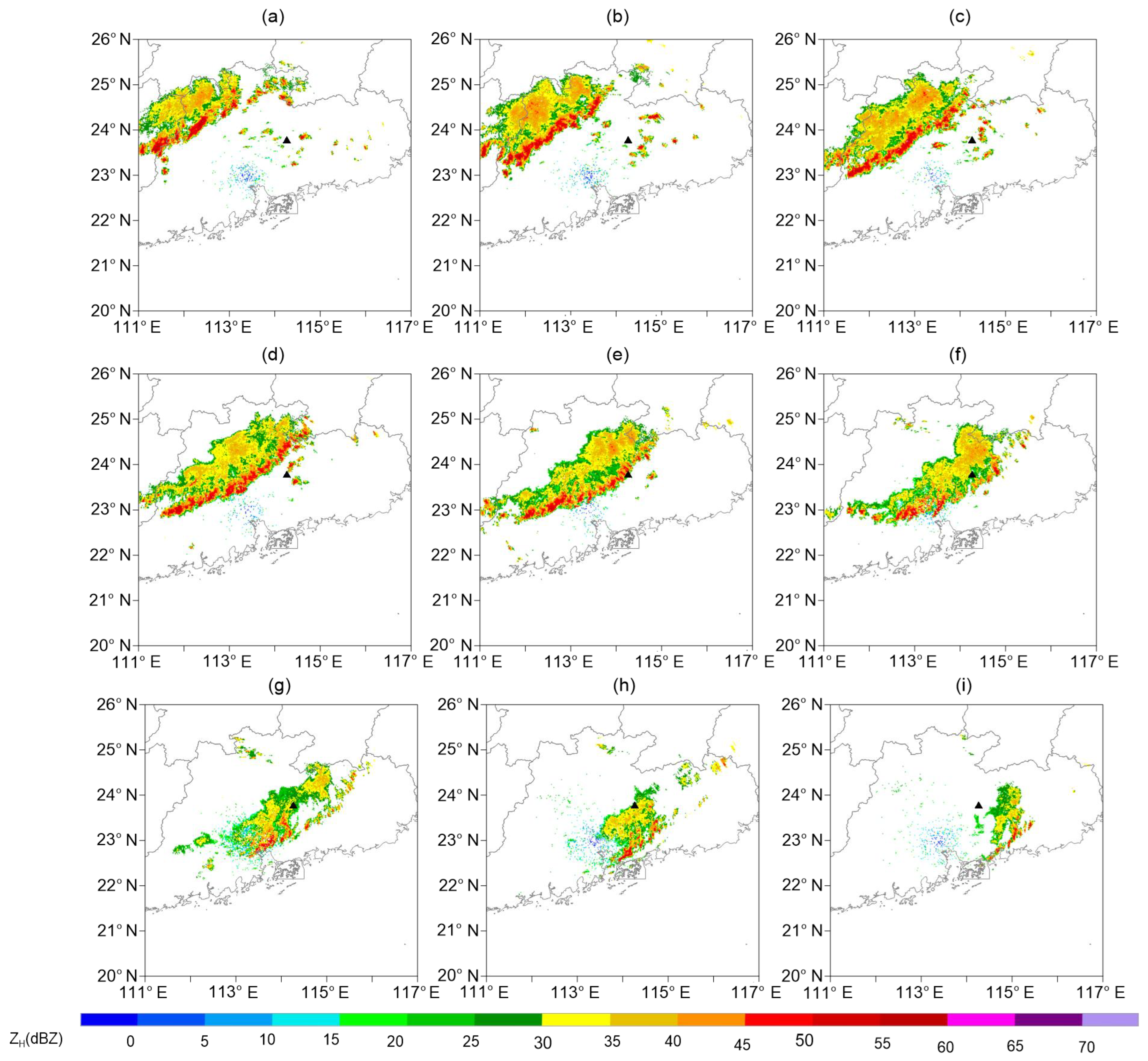
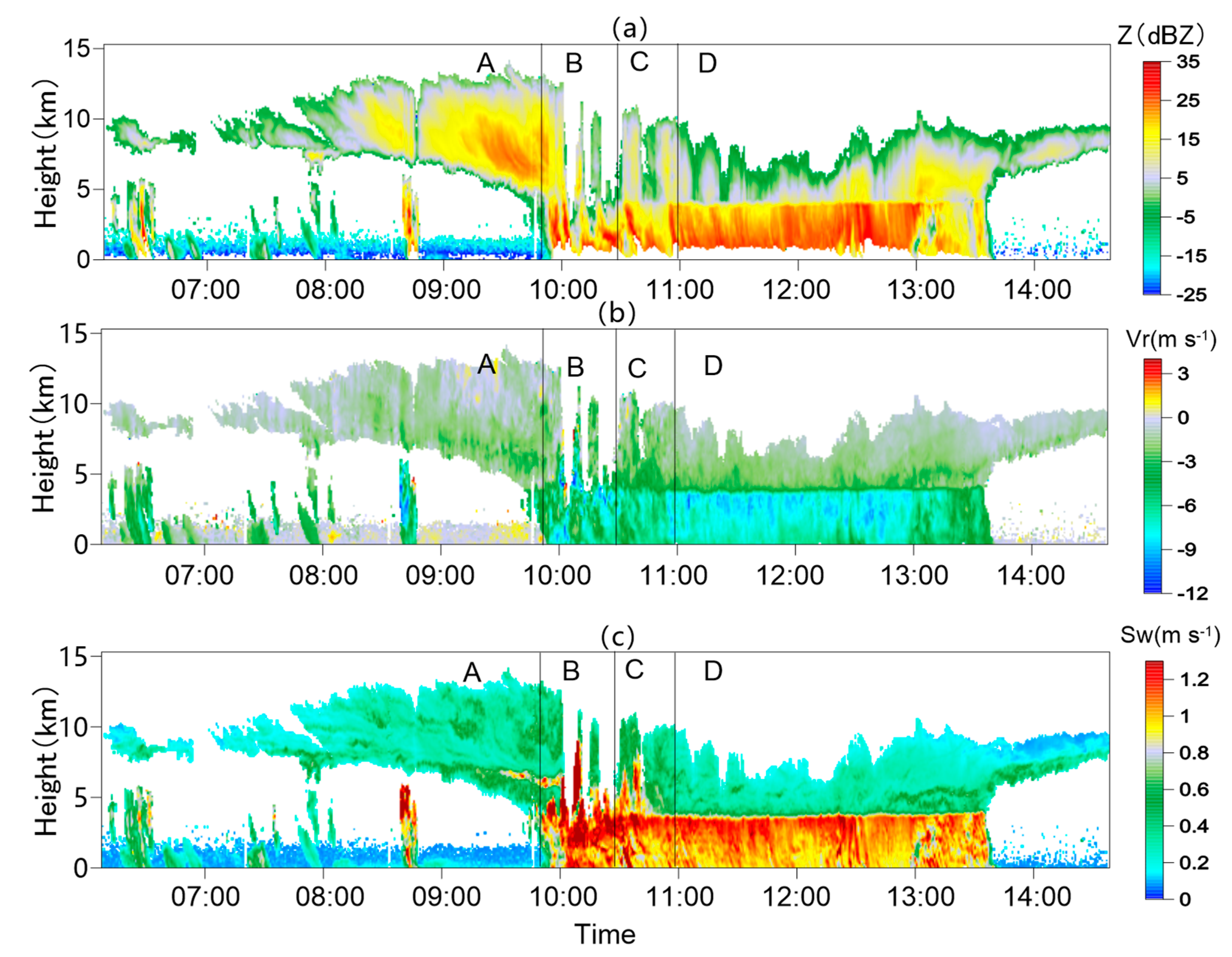
CR and PR detected cloud structures as the squall line passed, showing the evolution of the stages before passage (segment A), the strong convection time segment (segment B), the transition time segment (segment C), and the stratiform cloud time segment (segment D). The detection results showed that some local convection with falling rain inside and an upper layer altostratus cloud existed in segment A. The altostratus cloud was the blanket cloud extending from the front end of the squall line body. When the main body of the squall line passed by in segment B, strong convection and precipitation existed, with a reflectivity factor exceeding 35 dBZ and a velocity spectrum width exceeding 1.3 m s−1 detected by CR. As a result, intensive attenuation was caused by the heavy rain in the CR detection; thus, part of the echo in the upper layer could not be observed. According to the PR polarization parameters, Z of segment B was very high, with a maximum of 50 dBZ, and Zdr was 1–2, with the Kdp large value also representing large liquid water content. In segments C and D, the cloud and rain stabilized gradually, with descending cloud tops, stable precipitation, and a zero-layer bright band. Smaller Kdp values (less than 0.9) were distributed in the 0 °C layer, at approximately 3–5 km, which may have been caused by the melting of ice crystal particles. The strong attenuation is a limitation in the use of millimeter-wavelength radar.
(2)
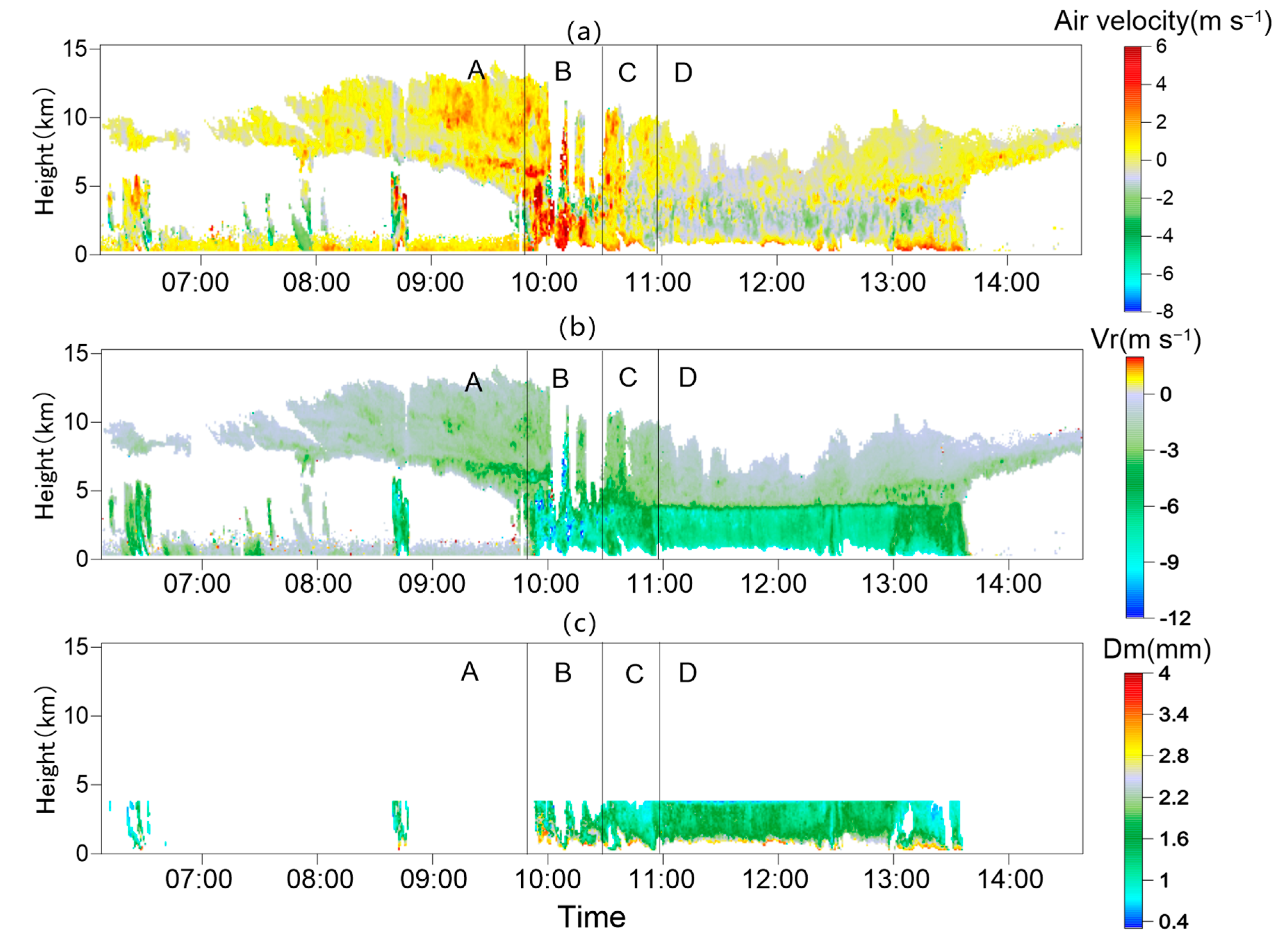
In the CR-retrieved vertical air velocity within the squall line in segment A, the downdraft was dominant in the local convection and a weak updraft existed in the higher-altitude altostratus clouds. In segment B, the strong upward speed under 5 km was significant, reaching more than 8 m s−1. Between segments C and D, the upward air velocity changed gradually to a wide range of weak downdrafts.
(3)
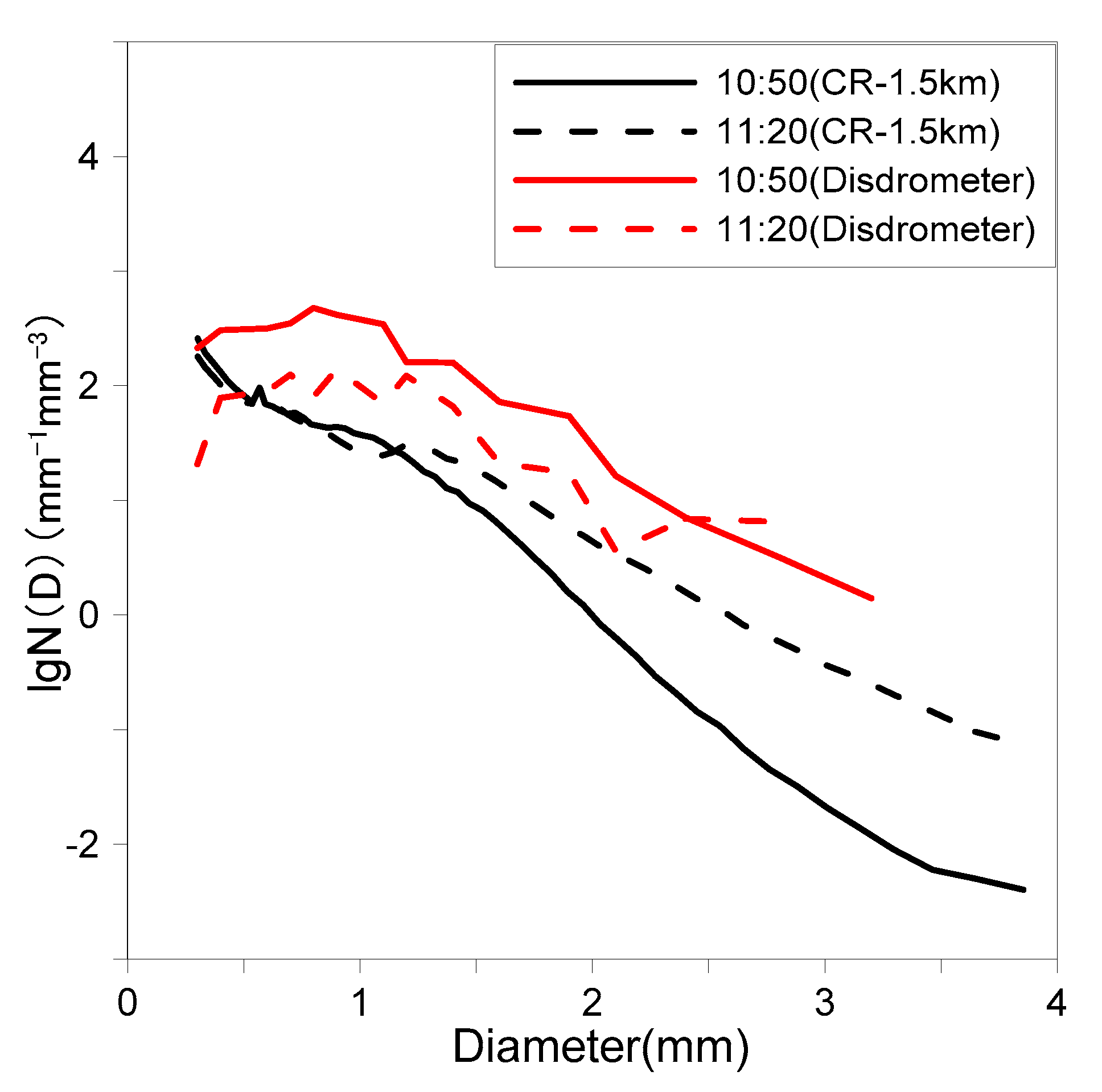
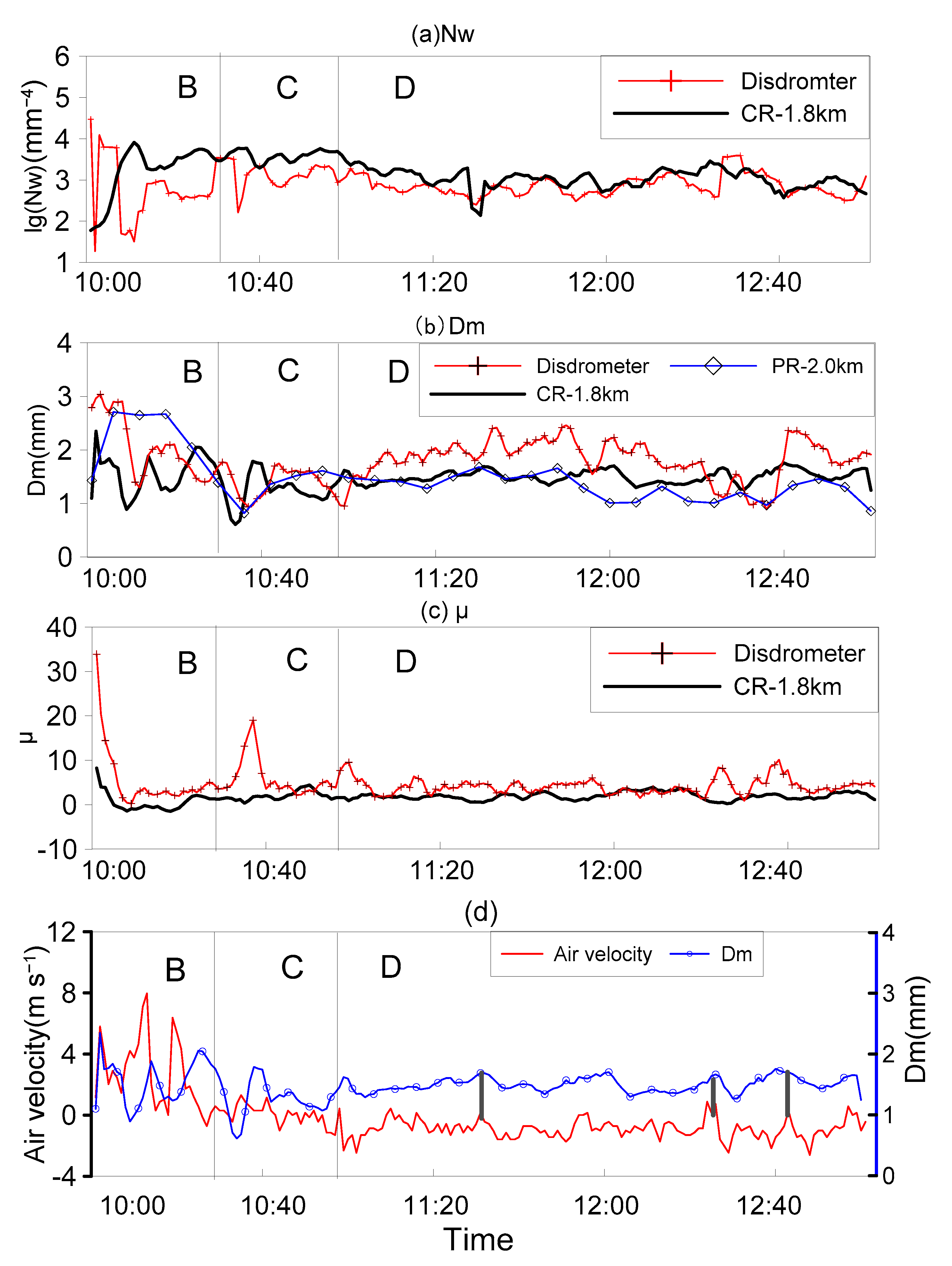
We calculated the CR data for DSD evolution during the passage of the squall line. Dm was almost entirely distributed within 1–2 mm at all heights. First, in the comparison of DSD by CR at 1.5 km and DSD data obtained on the ground, the retrieved DSD line was lower than the disdrometer in segment C, and the difference decreased between segments C and D. Second, DSDs were fitted using a normalized gamma distribution. In segments C and D, the Nw and μ values of the CR-retrieved DSD at 1.8 km showed good agreement with the ground data. The CR-retrieved Dm at 1.8 km was very close to the PR-retrieved Dm at 2 km; however, the Dm of the ground DSD was generally larger than both. Therefore, comparing with the DSD retrieved at around 2 km, the overall number concentration remained unchanged and Dm got larger on the ground, possibly reflecting the process of raindrop coalescence. Third, in segment B, CR-retrieved DSD parameters fluctuated greatly, but failed to reflect the characteristics of large raindrops, as shown by the disdrometer DSD parameters. Echo attenuation may have a significant influence on results retrieved in segment B.
(4)
In the comparison of the average vertical profiles of several quantities in segments B, C, and D, first, the CR-retrieved Dm decreased with height. The decrease of Nw and Dm with height in segments C and D were similar, which reflects the collision effect of falling raindrops. The changes were opposite in segment B, with Nw decreasing and Dm increasing as the height decreased. This indicates that raindrops underwent intense mixing and rapid collision and growth. Second, in segments B and C, the CR-retrieved Dm was approximately 0.5 mm smaller than the PR-retrieved Dm, and the distribution trends of the overlapping height range were similar. This is partly because of the Z difference of the two radars caused by the serious echo attenuation of CR. In segment D, the Dm values of the two radars within 2–4 km were consistent. Overall, the PR-retrieved Dm can verify the veracity of the CR-retrieved Dm. Third, from the mean vertical velocity profile of different segments, the larger rising velocity in the CR retrieval corresponded to the larger Dm, especially in segment C and D. The vertical velocity profile peak generated a larger Dm value.
As a whole, this study analyzed the microphysical structures of a squall line, providing the dynamic structure and hydrometeor distributions during each time interval and at different layers. Compared with other studies on weak cloud and precipitation using cloud radar, our study tried to analyze typical convective precipitation. Our analysis provided not only the comparison of DSD at ground and the CR-retrieved DSD, but also the vertical profiles of two radars’ retrieved parameters, verifying the credibility of the DSD and vertical air motion results. However, the echo attenuation may have a great influence on the retrieved results of the convective time segment. In future research, we plan to investigate the echo difference between CR and PR radar to make up for the retrieval error caused by such a difference.

Author Contributions

Conceptualization, N.M. and L.L.; methodology, N.M. and L.L.; software, N.M.; validation, L.L., Y.C., and Y.Z.; data curation, N.M.; writing—original draft preparation, N.M.; writing—review and editing, L.L., Y.C., and Y.Z. All authors have read and agreed to the published version of the manuscript.

Funding

This research was funded by the National Key Research and Development Program of China, grant number 2017YFC1501405, and the National Natural Science Foundation of China (42075092).

Institutional Review Board Statement

Not applicable.

Informed Consent Statement

Not applicable.

Acknowledgments

The authors want to give sincere thanks to the data and information of the field experiments organized by State Key Laboratory of Severe Weather, Chinese Academy of Meteorological Sciences.

Conflicts of Interest

The authors declare no conflict of interest.

References

  1. Houze, R.A.; Biggerstaff, M.I.; Rutledge, S.A.; Smull, B.F. Interpretation of Doppler weather radar displays of midlatitude mesoscale convective systems. Bull. Am. Meteorol. Soc. 1989, 70, 608–619. [Google Scholar] [CrossRef] [Green Version]
  2. Houze, R.A.; Smull, B.F.; Dodge, P. Mesoscale organization of springtime rainstorms in Oklahoma. Mon. Weather Rev. 1990, 118, 613–654. [Google Scholar] [CrossRef]
  3. Chong, M.; Amayenc, P.; Scialom, G.; Testud, J. A tropical squall line observed during the COPT 81 Experiment in west Africa. Part Ⅰ: Kinematic structure inferred from dual-Doppler radar data. Mon. Weather Rev. 1987, 115, 670–694. [Google Scholar] [CrossRef] [Green Version]
  4. Frankhuaser, J.C.; Barnes, G.M.; LeMone, M.A. Structure of a midlatitude squall line formed in strong unidirectional shear. Mon. Weather Rev. 1992, 120, 237–260. [Google Scholar] [CrossRef]
  5. Wang, T.C.C.; Lin, Y.K.; Shen, H.; Pasken, R.W. Characteristics of a subtropical squall line determined from TAMEX dual-Doppler data. Part Ⅰ: Kinematic structure. J. Atmos. Sci. 1990, 47, 2357–2381. [Google Scholar] [CrossRef] [Green Version]
  6. Roux, F. Retrieval of thermodynamic fields from multiple-Doppler radar data using the equations of motion and the thermodynamic equation. Mon. Weather Rev. 1985, 113, 2142–2157. [Google Scholar] [CrossRef] [Green Version]
  7. Pan, Y.J.; Zhao, K.; Pan, Y.N.; Wang, Y.P. Dual-Doppler analysis of a squall line in southern China. Acta Meteorol. Sin. 2012, 70, 736–751. [Google Scholar] [CrossRef]
  8. Wu, H.Y.; Chen, H.S.; Jiang, Y.F. Observation and Simulation Analyses on Dynamical Structure Features in a Severe Squall Line Process on 3 June 2009. Plateau Meteorol. 2012, 32, 1084–1094. (In Chinese) [Google Scholar] [CrossRef]
  9. Kollias, P.; Albrecht, B.A.; Marks, F. Why Mie? Accurate Observations of Vertical Air Velocities and Raindrops Using a Cloud Radar. Bull. Am. Meteorol. Soc. 2002, 83, 1471–1483. [Google Scholar] [CrossRef] [Green Version]
  10. Shupe, M.D.; Kollias, P.; Poellot, M.; Eloranta, E. On Deriving Vertical Air Motions from Cloud Radar Doppler Spectra. J. Atmos. Ocean. Technol. 2008, 25, 547. [Google Scholar] [CrossRef] [Green Version]
  11. Tridon, F.; Planche, C.; Mroz, K.; Banson, S.; Battaglia, A.; Baelen, J.V.; Wobrock, W. On the Realism of the Rain Microphysics Representation of a Squall Line in the WRF Model. Part I: Evaluation with Multifrequency Cloud Radar Doppler Spectra Observations. Mon. Weather Rev. 2019, 147, 2787–2810. [Google Scholar] [CrossRef] [Green Version]
  12. Liu, L.P.; Xie, L.; Cui, Z.H. Examination and application of Doppler spectral density data in drop size distribution retrieval in weak precipitation by cloud radar. Chin. J. Atmos. Sci. 2014, 38, 223–236. (In Chinese) [Google Scholar] [CrossRef]
  13. Peng, L.; Chen, H.B.; Li, B. A case study of deriving vertical air velocity from 3-mm cloud radar. Chin. J. Atmos. Sci. 2012, 36, 1–10. (In Chinese) [Google Scholar] [CrossRef]
  14. Hildebrand, P.H.; Sekhon, R.S. Objective determination of the Noise Level in Doppler Spectra. J. Appl. Meteorol. 1974, 13, 808–811. [Google Scholar] [CrossRef] [Green Version]
  15. Ma, N.K.; Liu, L.P.; Zheng, J.F. Application of Doppler spectral density data in vertical air motions and drop size distribution retrieval in cloud and precipitation by Ka-band Millimeter Radar. Plateau Meteorol. 2019, 38, 325–339. (In Chinese) [Google Scholar] [CrossRef]
  16. Gossard, E.E. Measurement of cloud droplet size spectra by Doppler radar. J. Atmos. Ocean. Technol. 1994, 11, 712–726. [Google Scholar] [CrossRef] [Green Version]
  17. Testud, J.; Oury, S.; Black, R.A.; Amayenc, P. The Concept of “Normalized” Distribution to Describe Raindrop Spectra: A Tool for Cloud Physics and Cloud Remote Sensing. J. Appl. Meteorol. 2001, 40, 1118–1140. [Google Scholar] [CrossRef]
  18. Cao, Q.; Zhang, G.; Schuur, T.; Ikeda, K. Analysis of Video Disdrometer and Polarimetric Radar Data to Characterize Rain Microphysics in Oklahoma. J. Appl. Meterol. Climatol. 2008, 47, 2238–2255. [Google Scholar] [CrossRef] [Green Version]
Figure 1. Radar echo of the squall line determined by the dual-polarization S-band weather radar of Guangzhou from 0600 to 1400 UTC on 6 May 2016: (a) 0600, (b) 0700, (c) 0800, (d) 0900, (e) 1000, (f) 1100, (g) 1200, (h) 1300, and (i) 1400 (the black triangle marks the position of the Ka-band cloud radar).
Atmosphere 12 00348 g001
Figure 2. Time–height cross-sections of the squall line echoes observed by CR on 6 May 2016 in precipitation mode: (a) reflectivity factor Z (unit: dBZ), (b) radial velocity Vr (unit: m s1), and (c) velocity spectrum width Sw (unit: m s1). Different stages of the squall line are divided by black solid lines, with the time segment before the passage of the squall line, the strong convection time segment, the transition time segment, and the stratiform time segment labeled A, B, C, and D, respectively.
Atmosphere 12 00348 g002
Figure 3. Time–height cross-sections of the squall line echoes observed by PR on 6 May 2016: (a) reflectivity factor Z (unit: dBZ), (b) differential reflectivity factor Zdr (unit: dBZ), (c) correlation coefficient ρhv, and (d) specific differential phase Kdp (unit: °/km). Different stages of the squall line are divided by black solid lines, and the time segment before the passage of the squall line, the strong convection time segment, the transition time segment, and the stratiform time segment are labeled A, B, C, and D, respectively.
Atmosphere 12 00348 g003
Figure 4. Cloud radar retrievals of the squall line on 6 May, 2016: (a) Vertical air velocity (unit: ms−1), (b) free-falling velocity of raindrops in still air (unit: ms−1), and (c) weighted average diameter (unit: mm). Different stages of the squall line are divided by black solid lines, and the time segment before the passage of the squall line, the strong convection time segment, the transition time segment, and the stratiform time segment are labeled A, B, C, and D, respectively.
Atmosphere 12 00348 g004
Figure 5. Comparison of retrieved DSD at 1.5 km and disdrometer-obtained DSD during segments B (convective clouds), C (transition clouds), and D (stratified clouds) (unit: mm−1 m−3).
Atmosphere 12 00348 g005
Figure 6. Time series of the three DSD fitting parameters at ground level retrieved by the disdrometer and at 1.8 km retrieved by CR during 0947–1300 UTC on 6 May 2016: (a) Nw (unit: mm−1 m3), (b) Dm (unit: mm), and (c) μ. Dm time series of PR at 2 km is represented by the blue line in (b). Time series of Dm and vertical air velocity retrieved by CR are shown in (d), and the gray lines connect the peak values. Different stages of the squall line are divided by black solid lines, with the time segment before the passage of the squall line, the strong convection time segment, the transition time segment, and the stratiform cloud time segment labeled A, B, C, and D, respectively.
Atmosphere 12 00348 g006
Figure 7. The average profiles of several quantities in segments B, C, and D, including the reflectivity factor, polarization parameters of PR, vertical air velocity, and DSD parameters by CR. (a,c,e) show the Zdr, Kdp, Dm, vertical air velocity, and Nw profiles of segments B, C, and D, respectively, and (b,d,f) show the reflectivity factor profiles of PR and CR in regions B, C, and D, respectively.
Atmosphere 12 00348 g007
Table 1. Main specifications of the cloud radar.
ParameterCloud Radar
Transmitting frequency33.4 GHz
Wavelength8.5 mm
3 dB beam width0.3°
Range resolution30 m
Temporal resolution3 s
Nyquist velocity range−18.54~18.54 m·s−1
Height range0~15.3 km
Primary detection objectNonprecipitation clouds, weak precipitation clouds
Detecting elementsBase data, Doppler spectrum
Detection modeVertical pointing, three detection modes
Table 2. Main specifications of the S-band radar.
ParameterS-Band Radar
Antenna diameter8.54 m
Antenna gain45.31 dB
Beam width<0.98°
First side lode<−30 dB
Wavelength10.3 cm
Operating modeSimultaneous horizontal and vertical transmission and reception
Minimum detectable power−117.8 dBm
Volume scan modeVCP21 (9 tilts)
Range resolution0.25 km
Table 3. Main specifications of HSC-PS32.
ParameterHSC-PS32
Sensor typeLaser transmitter
Wavelength785 nm
Sensor componentsRed laser shooting
Weather type22 classes (no rain, fog, rain, snow, drizzle, hail, etc.)
Measurement area54 cm
Measurement rangeParticle size: 0~25 mm
Velocity: 0~20 m s−1
Rain rate: 0.001~1200 mmh−1
Height range0~15.3 km
Measurement rangeNonprecipitation clouds, weak precipitation clouds, weak precipitation
Detection principleA combination of extinction with forward
scattering
Working temperature−40~+60 °C
Storage temperature−50~+70 °C
Data communicationsWireless communications (GPRS)
Publisher’s Note: MDPI stays neutral with regard to jurisdictional claims in published maps and institutional affiliations.

