Article

The Neural Network Assisted Land Use Regression

by
Jan Bitta
1,2,
Vladislav Svozilík
1,2,* and
Aneta Svozilíková Krakovská
3,4
1
Laboratory of Information Technologies, Joint Institute for Nuclear Research, Moscow Region, 141980 Dubna, Russia
2
Faculty of Materials Science and Technology, VSB—Technical University of Ostrava, 70800 Ostrava-Poruba, Czech Republic
3
Faculty of Mining and Geology, VSB—Technical University of Ostrava, 70800 Ostrava-Poruba, Czech Republic
4
Frank Laboratory of Neutron Physics, Joint Institute for Nuclear Research, Moscow Region, 141980 Dubna, Russia
*
Author to whom correspondence should be addressed.
Atmosphere 2021, 12(4), 452; https://doi.org/10.3390/atmos12040452
Submission received: 13 March 2021 / Revised: 30 March 2021 / Accepted: 30 March 2021 / Published: 1 April 2021
(This article belongs to the Special Issue Advances in Air Quality Data Analysis and Modeling)

Abstract

:
Land Use Regression (LUR) is one of the air quality assessment modelling techniques. Its advantages lie mainly in a much simpler mathematical apparatus, quicker and simpler calculations, and a possibility to incorporate more factors affecting pollutant concentration than standard dispersion models. The goal of the study was to perform the LUR model in the Polish-Czech-Slovakian Tritia region, to test two sets of pollution data input factors, i.e., factors based on emission data and pollution dispersion model results, to test regression via neural networks and compare it with standard linear regression. Both input datasets, emission data and pollution dispersion model results, provided a similar quality of results in the case when standard linear regression was used, the R2 of the models was 0.639 and 0.652. Neural network regression provided a significantly higher quality of the models, their R2 was 0.937 and 0.938 for the factors based on emission data and pollution dispersion model results respectively.

1. Introduction

1.1. Air Pollution

Air pollution is an undesirable state of the environment caused by the emission of pollutants from various pollution sources to the air. A pollutant is defined as any substance that negatively affects human health, ecosystems or properties [1,2]. The overall imbalance in the environment has increased over the years. Sources of pollution can be classified as natural and anthropogenic. Concentrations emitted by natural sources appear as a natural background and are not influenced by human activities [1]. Anthropogenic pollution is caused by human activities, and its origin is bound to human settlements. Anthropogenic pollution, unlike natural pollution, is influenceable. Common air pollution pollutants are particulate matter (PM10 and PM2.5), nitrogen oxides, carbon monoxide, sulphur dioxide, benzo[a]pyrene, persistent organic pollutants (POPs), etc., [3]. This article deals with PM10. PM10 are solid or liquid (aerosol) particles of 10 μm or less in diameter, compound from various organics, sulfates, nitrates, ammoniac salts, soot, mineral particles, metals, bacteria, pollen and water [1].

1.2. Air Pollution Modelling

Air pollution monitoring is a standard tool for the air pollution assessment. In the Czech Republic, it is supposed to be the main tool for air monitoring and research in accordance with Czech Act no. 201/2012 Coll. Air pollution concentrations are regulated in respect to both acute effects of pollution exposure (short-term averages) and the effects of chronic air pollution exposure represented by yearly averages. This approach was implemented from the EU Legislation Act on Ambient Air Quality and Cleaner Air for Europe [4] and is universal for the EU countries. The given study focuses on the chronic part of the air pollution effect represented by yearly averages.
The disadvantage of pure air pollution monitoring is that measurements can provide information about concentrations only at specific measurement points. For effective air pollution management, it is better to have continuous information about the distribution in the study area. Mathematical air pollution dispersion modelling is a suitable method to acquire the concentration distribution of air pollution in the study area.
Mathematical models utilized in the air quality assessment and management can be classified by the model type as [5]:
  • empirical models,
  • Gaussian models,
  • numerical models,
  • physical models.
Physical models are a smaller physical representation of a real situation that they represent and allow studying. Numerical models are a category of models based on general formulas and algorithms of computational fluid dynamics. These model categories are not considered in the study.
Empirical models are based on in situ measurements and observations. They use various data analysis techniques to create a model describing the phenomenon under study. Empirical models are usually much simpler, require less computational power, and are easier to work with. Their biggest disadvantage is that they are site and time specific. Their scope is limited by the data they are based on. A difference in data location or a time period results in different models constructed. Land Use Regression (LUR) models belong to the empirical model category.

1.3. Gaussian Models

Gaussian dispersion modelling is based on the assumption of continuous leakage of pollution from a pollution source and subsequent dispersion of pollutants in a constant homogeneous wind speed field without spatial limiting conditions. The dispersion of pollutants occurs in the wind direction due to convection and in the direction perpendicular to it due to diffusion, which is caused by atmospheric turbulence and expressed statistically using the (Gaussian) normal distribution [6]. Spatial limiting conditions, such as the effect of terrain, are included in the calculation using coefficients [7]. Input data of Gaussian models are terrain data, meteorological data, the characterization of pollution sources, and a mesh of reference points. Input data characterize an average situation during the modelled period [8].
Gaussian models work with a reasonable degree of air pollution dispersion process abstraction. Therefore, it is possible to describe the relationship between the concentrations at the reference point and the source using an easily enumerable mathematical formula. Simultaneously, abstraction imposes smaller requirements on the input data and time consumption of evaluation. Therefore, Gaussian models are widely used for air pollution modelling in widespread areas. Among the Gaussian air pollution models preferred by the EPA are Industrial Source Complex (ISC) [9], CALPUFF [10], CALINE3 [11], AERMOD [12], and others. Gaussian models preferred by the Czech legislation are SYMOS’97 [13], AEOLIUS [14] and ATEM [15]. These models provide steady-state results describing air pollution concentrations in the study area and time interval.

1.4. Land Use Regression

Models based on Land Use Regression belong to the category of empirical models. LUR can be treated as an independent air pollution modelling method. This kind of model is based on the principle that concentrations at a specific location depend on the characteristics of the surrounding environment, especially the characteristics that affect the intensity of emissions and rate of dispersion and deposition. Modelling itself is performed on the basis of the regression model describing the influence of relevant environmental and spatial characteristics, i.e., input factors [16,17]. The model is composed of regression equations that include the relationship between input factors and substance concentrations at monitoring sites. The resulting formula can be used to predict concentrations over the whole area represented by point measurements.
LUR models are not tied to any time or spatial resolution. They are used in a variety of time intervals from short-term campaigns to long-term averages at fixed pollution monitoring sites. The spatial resolution of LUR models can vary from hyper-local urban areas to regional or country level models.
Most LUR models deal with linear regression [18]. Linear regression describes the relationship between the variables x and y, where the values of x (x can be a scalar or a vector representing a set of input values) are assumed to be independent variables and measured without errors. Linear regression consists of two variables connected by a linear function [19]. The dependent random variable represents the value of y under investigation. It is assumed that the variable y is a linear function of x. The coefficient of determination (R2) is used to evaluate the relationship between these variables [20].
LUR itself is especially useful in areas that are difficult to monitor or have an unsatisfactory density of the monitoring station mesh. Therefore, LUR air pollution modelling is used for assessment all over the world, especially in Europe, America, Australia, and Asia.
Van den Bossche et al. [21] used mobile monitoring to gather data at a high spatial resolution in order to build LUR models for the prediction of annual average concentrations of black carbon (BC). The overall prediction was low due to the input uncertainty and lack of predictive variables. The authors highlighted the use of independent data to validate and exclude those data during variable selection in the model building procedure and the importance of using an appropriate cross-validation scheme to estimate the predictive performance of the model. LASSO, the regularized linear model, performed slightly better than the classical supervised approach, and the nonlinear SVM technique did not show significant improvement over the linear model. The generalization of the LUR model to areas where no measurements were made was limited, especially when predicting absolute concentrations.
Lee et al. [22] developed LUR models for particulate matter in the Taipei Metropolis with a high density of roads and strong activities of industry, commerce, and construction. It was possible to achieve R2 values of 95% (PM2.5), 96% (PM2.5 absorbance), 87% (PM10), and 65% (PMcoarse). Local traffic, construction, residential land use, and industrial sources were identified as the causes of PM2.5 pollution. A variable representing the river vicinity decreased PM2.5 pollution. PM2.5 absorbance levels were boosted by local traffic, commercial and industrial land use. Increased concentrations of PMcoarse were caused by elevated motorways.
LUR input data have a spatial character. Geographic information systems are a suitable tool for processing and management, especially when using remote sensing data. Hsu et al. [23] used GIS and remote sensing to develop ten regression models for the PM2.5 bound compound concentration based on measurements of a six-year period. The regression models included NH 4 + , SO 4 2 , NO 3 , OC, EC, Ba, Mn, Cu, Zn, and Sb. The authors managed to explain the variance (R2) of the LUR models in the range between 0.60 and 0.92. In the course of the study, they were able to successfully estimate the fine spatial variability of PM2.5 and its compounds in Taiwan. Traffic distribution, industrial areas, greenness, and culture-specific PM2.5 sources, such as temples, were used as inputs. The main variables determined by the LUR model that affect PM2.5-bound concentrations are traffic, industrial areas, and greenness.
The study Wu et al. [24] assesses the influence of surrounding greenness on the concentrations caused by local culture-specific emission sources (Chinese restaurants and temples) within a city of Taipei using LUR modelling. Correlation analysis of the LUR PM2.5 model was carried out. A strongly negative correlation (r: −0.71 to −0.77) between NDVI was detected. Temples (r: 0.52 to 0.66) and Chinese restaurants (r: 0.31 to 0.44) were positively correlated with PM2.5 concentrations. The result was confirmed using a cross-validation test with the result R2 of 0.90 and external validation R2 of 0.83, and with the adjusted model R2 of 0.89.

1.5. Artificial Neural Networks

Artificial neural networks (ANNs) are a mathematical abstraction of biological processes that constitute animal brains. An ANN consists of a set of nodes and neurons, which are interconnected. It loosely simulates the neurons of animal brains. Synapses are represented by these connections. Each neuron receives signals via connections, processes them, and signals further via connections. The signal is a real number. In each neuron, the input signals are summed and transformed using some nonlinear function (activation function). The result is an output signal of the neuron. Each input connection has a weight set, which increases or decreases the importance of the signal. The neuron can also have a bias property that represents the sensitivity of the neuron to the signal. The bias value is added to the input signal. Neurons are usually aggregated into layers. The layers can have different activation functions. In each neural network, the signal is propagated from the input receiving layer (input layer) to the output layer, which provides the output signal through one or more layers of neurons. The signal can be one-directional or contain loops McLachlan et al. [25]. Neural networks can be trained via sets of examples consisting of pairs that combine inputs and desired results. From a mathematical point of view, training is an optimization process that optimizes the performance of the neural network. The performance is usually defined as the difference between the desired results and neural network outputs. Independent variables of the optimization are the weights and biases of the neural network. The adjustment of the weights and biases gives increasingly more accurate results. The training of the network is terminated after a sufficient number of adjustments. This process is called supervised learning. There are also types of neural networks that are trained on data not containing the desired results. This process is called unsupervised learning.
Network training is a time-consuming process demanding a lot of computational power. Once the training process is completed, the neural network is able to recall the output value when provided with an input dataset. Mathematically, this is an enumeration of an explicit mathematical formula, a quick and simple operation.
2. Methodology

2.1. Gaussian Models

The Analytical Dispersion Modelling Supercomputer System (ADMOSS) was developed at the VSB—Technical University of Ostrava (VSB-TUO) to perform air pollution modelling in widespread areas [26]. The ADMOSS is based on a combination of geographic information systems (GIS), a mathematical model of air pollution dispersion, and parallel computer clusters. The Modelling methodology implemented in the ADMOSS is the Gaussian model SYMOS’97 recommended by the Czech legislation [27]. The ADMOSS is independent of the modelling methodology and able to run with other models of the same class. Studies (Air Silesia [28], AIR PROGRES CZECHO-SLOVAKIA [29], AIR TRITIA [30]) focusing on air pollution modelling and assessment in the Czech-Polish-Slovak borderland were carried out using the ADMOSS. The study is based on the Gaussian modelling results of the AIR TRITIA project.

2.2. Input Factors of the Land Use Regression

Three groups of factors, i.e., emission factors, results of air pollution dispersion modelling, and land cover factors, were considered in the study. Each modelling result factor was read out as a value at pollution monitoring sites. Factors of land cover and factors representing emission were calculated in a similar manner. Based on the experience from Bitta et al. [31], all factors representing land cover and emission were enumerated as weighted averages, where the weights were defined by the estimated probability of the wind direction.
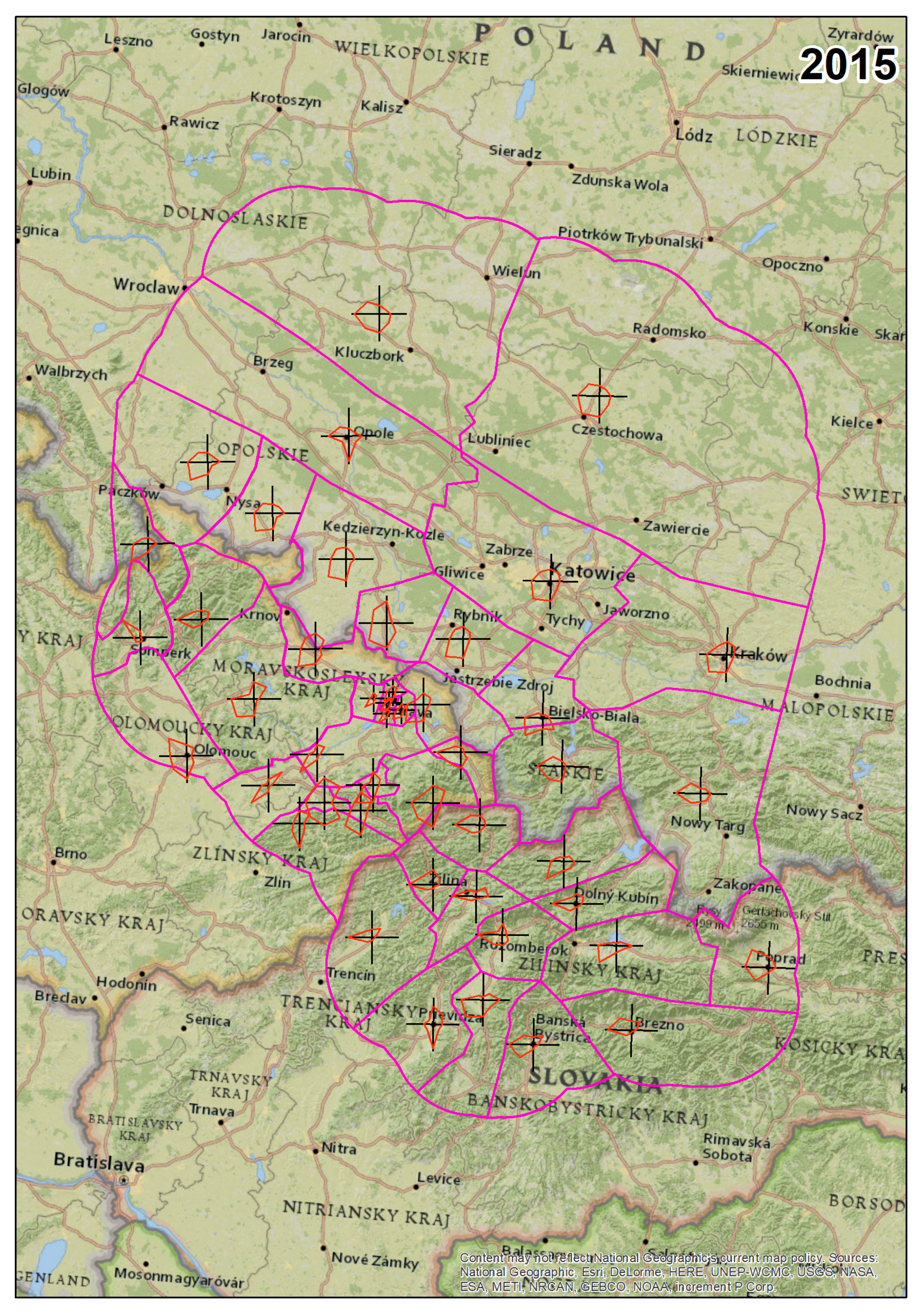
The whole area of interest was divided into 46 areas, the division was performed with respect to the terrain configuration. Each area had its own unique meteorological dataset. Buffer zones around the monitoring stations were divided into eight slices representing eight wind directions. The factors were calculated as wind direction probability weighted averages of the factors calculated in the slices. The outlines of division polygons and wind direction probability graphs are visualized in Figure 1.
All factors considered in the study are listed in Table 1. Tests which buffer perimeters are the most representative for the LUR were performed in the study in Section 4.1.

2.3. Neural Network-Based Regression

Neural networks with supervised learning can be utilized as a universal regression technique, an alternative to standard statistical methods. In the case of the LUR model, the set of input factors represents input data, and the pollutant concentration is the desired output. The neural network is trained to provide the desired results from a given list of input factor values.
When neural networks are used for such a task, there is a severe risk of overfitting. Overfitting is the product of analysis that corresponds too closely or exactly to a particular set of data and, therefore, may fail to fit additional data or reliably predict future observations (Figure 2).
We limited the maximal number of input factors to five and used the five-fold cross-validation technique to assess the suitability of the current dataset selection and neural network configuration to avoid overfitting. k-fold cross-validation is the technique that splits the initial data sample into k of equally sized subsamples. One subsample is kept for model testing and the remaining k 1 subsamples are training data. The training process is repeated k-times, each data subsample is once used as test data. The performance of the neural network is represented by the average performance of k trained neural networks [25].
For the sake of analysis, we used multilayer perceptron (MLP) neural networks. An MLP is a class of feedforward ANNs. It is a one-directional neural network consisting of three layers of neurons—the input layer, the hidden layer, and the output layer [32]. In the experiments, we used MLPs with the hidden layer, in which the number of neurons ranged from 1 to 30, and there were two possible activation functions—the logistical function and hyperbolic tangent.
To determine the best neural network configuration for each group of the selected factors, we tested all possible neural network configurations with five different random five-fold cross-validations. That resulted in the need to train 1500 neural networks and compare their performance for each combination of the hidden layer size and activation function. The performance parameter was the R 2 estimate based on average R 2 of cross-validation neural networks. When the optimal neural network configuration was determined, the final network with those parameters was trained on the whole dataset. The R 2 performance value of this neural network represents the quality of prediction based on the selected input factors.
A neural network-based LUR model was developed to estimate spatial and temporal variability of nitrogen dioxide (NO2). At first, the standard LUR model was elaborated to identify significant variables. Secondly, the deep neural network algorithm was applied on the LUR results to fit the model for predicting concentrations. Lautenschlager et al. [33] focus on the development of the OpenLUR platform. This platform consists of the LUR modelling technique combined with machine learning and open datasets.
The study performed by Alam and McNabola [34], extending the typical LUR approach with ANNs. At first, the average daily PM10 concentrations of Vienna and Dublin were delivered using the concept of multiple linear regression (MLR) modelling. Secondly, an ANN was used to manage the input variable nonlinearity. The best result of R2 = 66% for Vienna and 51% for Dublin was reached owing to the ANN.

3. Data Sources

2015 data were used in the study. The study area is the area of interest of the Air Tritia project [35]. The Air Tritia project focuses on air quality modelling and assessment. Emission and pollution monitoring data were collected and published in this project. The Tritia region consists of two Polish voivodships (Silesian, Opole), the Moravian-Silesian region in the Czech Republic and the Žilina region in Slovakia. Figure 3 demonstrates the position and size of the study area.
The level of air pollution was determined by vast hard coal deposits of the Upper Silesian Basin, which has been mined since the 18th century. The presence of coal enabled the growth of industries by using coal as a source of energy or as feedstock (coal mining, coal processing, steel production, industrial chemistry), downstream industries (e.g., machine industry) and coal heat and electricity production (utility, C&I and domestic scale). The combination of industrial production services, required by densely populated surrounding urban settlements, and the unfavorable basin-like terrain configuration are the cause of severe air pollution. The EEA marks the Tritia region with a population of approximately 7.5 million inhabitants as one of the most air polluted regions of the EU (Figure 4). The most problematic pollutants are particulates (PMx), PAH (polyaromatic hydrocarbons), and heavy metals (Hg, Cd, As) [36].

3.1. Air Pollution and Meteorological Data

Pollution monitoring data consist of yearly averages of PM10 (Figure 3) in 2015, collected from all pollution monitoring sites in the Tritia region. The values and site locations were obtained from yearbooks of the Czech Hydrometeorological Institute [38], the Slovakian Hydrometeorological Institute [38] and Inspectorates for Environmental Protection of the Silesian and Opole Voivodships [39,40]. There were 47 air pollution monitoring stations measuring the PM10 concentration in the study area. Yearly average values are presented in Table A1.
Meteorological data were obtained from the Air Tritia project dataset [41].

3.2. Emission Data

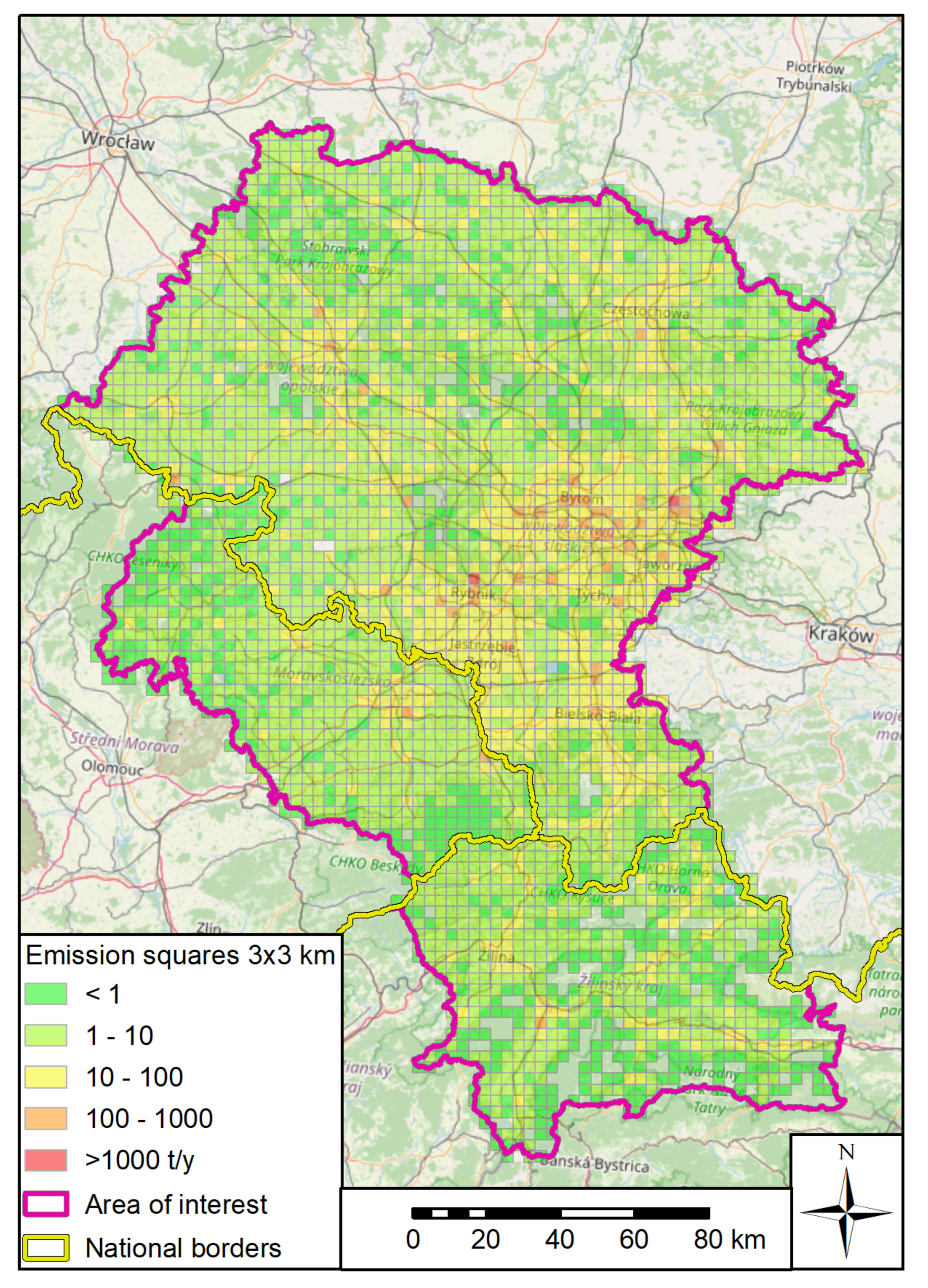
Emission data were obtained from the emission database provided by the Air Tritia project. The data were divided by the country of origin (Czech–Polish-Slovak) and type of pollution source (industrial, domestic heating, car traffic). Industrial sources were represented as point sources, and the input data contained following parameters: position, average emission flow, height, exhaust diameter, speed, volume flow, and the temperature of exhaust gases. Domestic heating was represented by area sources, which were squares of a 200-m size containing a position, average emission flow, and height. Car traffic sources were modelled as linear sources with a length ≤50 m containing a line description, average emission flow, and height. Brief emission statistics are presented in the following table (Table 2) and emission squares (Figure 5) [30].

3.3. Gaussian Model Results

The results of the Gaussian model were obtained from the Air Tritia project. The long-term SYMOS’97 model was used in the project. Meteorological conditions were standardized by the wind speed (low, medium, strong), wind direction (eight directions + calm), and atmospheric stability (Bubník–Koldovský classification, five classes) in the long-term model. Each combination of the meteorological parameters was calculated separately, and the annual average concentration was calculated as a mean of those values weighted by the probability of occurrence of such weather conditions. The emission data entered modelling in the form described in the section above [13,42].

3.4. Land Use Data

Land use data were represented by data from vector topographical datasets, namely, ZABAGED (CZ), BDOT (PL), ZBGIS (SK), which are all available at a 1:10,000 map scale CUZK [43], GUGiK [44] and GKU [45]. There were five kinds of land cover used for analysis, i.e., built-up areas, forested areas, grass-covered areas, water bodies, and open soil agricultural areas.

4. Experiments and Results

The modelling experiment was structured according to the following flowchart (Figure 6).
The first step of the modelling experiment was to calculate possible input factors based on emission data, land cover data, and Gaussian model results. The number of possible input factors for LUR needed to be reduced. For this reason, the second step of the experiment was factor preselection. When a proper set of possibly eligible factors was selected, LUR modelling followed.
Four sets of LUR models were constructed. Standard LUR models using linear regression were constructed for each combination of five or less input factors. The first set of input factors consisted of emission factors and land cover factors, and the second set of input factors comprised Gaussian model factors and land cover factors. Neural network-assisted LUR models were also developed for the same two groups of input factors mentioned above. Those models replaced the linear regression of LUR models with nonlinear regression provided by the neural network.
The best models were selected from each of the four calculated model groups, which represented the best available result of the combination of the input factor group and regression technique. The R 2 value of the models was chosen as the quality parameter for the result of each model.
All calculations and data analysis were performed in the Python 3.4 programming language. The pandas module was used for table data handling, the statmodels module was applied for basic statistical analysis, the matlibplot module was used for graph generation, and sklearn was applied for neural network analysis. All the modules above are parts of the Anaconda distribution of the Python language Anaconda [46], which was utilized for calculations. arcpy is the API of the ArcGIS Pro 2.6 software, which enables spatial analysis and map generation in the Python environment.
The modelling experiment entailed a large number of mathematical computations, which were significantly accelerated due to parallel computing on the CESNET [47] Metacentrum and the “Govorun” supercomputer JINR [48], where hundreds of neural networks could be trained simultaneously.

4.1. Factor Preselection

It was necessary to determine the best buffer zone perimeter for each emission and land cover factor. Analysis based on Spearman correlation coefficients was used. Factor values were calculated for distance perimeters ranging from 200 to 10,000 m with a 200 m step. Spearman’s correlation between each factor and the 2015 yearly average PM10 concentration at the monitoring sites was calculated (Figure 7). The best perimeters used in further analysis were the distances at which Spearman’s correlation had its local or global maximum.
Table 3 lists the selected factors and the best perimeters. There are also factors representing the model results included. The factors were read out from the model results at locations of the monitoring stations.

4.2. Linear Regression-Based Land Use Regression

Linear regression LUR models were developed using three different input factor groups, namely, emission factors, land cover factors (Table 3), and Gaussian model result factors. All the following models were limited to a maximum of five input factors to avoid overfitting during linear regression calculations on the dataset containing 47 monitoring sites. At first, models containing any subset of emission and land cover factors were tested (Figure 8). There were 1585 linear models tested. The quality of the models was determined by the coefficient of determination of the model ( R 2 ).
The best model found was a model containing the following factors: industrial sources in a 2000 m distance, car traffic in a 1000 m distance, built-in land in an 8000 m distance, forested area in a 400 m distance and grass covered land in a 5000 m distance. This model (Figure 9) has R 2 = 0.639 and the formula:
PM 10 = 32.6237 + 0.0212 I N 2000 + 0.4823 C A R 1000 + 0.2294 B L D 8000 0.1133 G R S 5000 0.0965 F R S 400
Secondly, the linear model was selected among linear models that were constructed using Gaussian model results for the industrial source ( M O D I N ), domestic heating ( M O D D H ), and car traffic ( M O D C A R ) and land cover factors. 465 models containing up to six input factors were constructed. The quality of the models was also determined by their coefficient of determination ( R 2 ) (Figure 10).
The best model found was a model containing the following factors: built-in areas in an 8000 m distance, forested area in a 400 m distance, grass covered land in a 5000 m distance, and all three Gaussian model results (Figure 11). This model has R 2 = 0.652 and the formula:
PM 10 = 28.7064 + 0.2457 B L D 8000 0.0870 F R S 400 + 0.0459 S O I L 5000 + 2.9565 M O D I N + 2.6991 M O D C A R

4.3. Neural Network-Assisted Land Use Regression

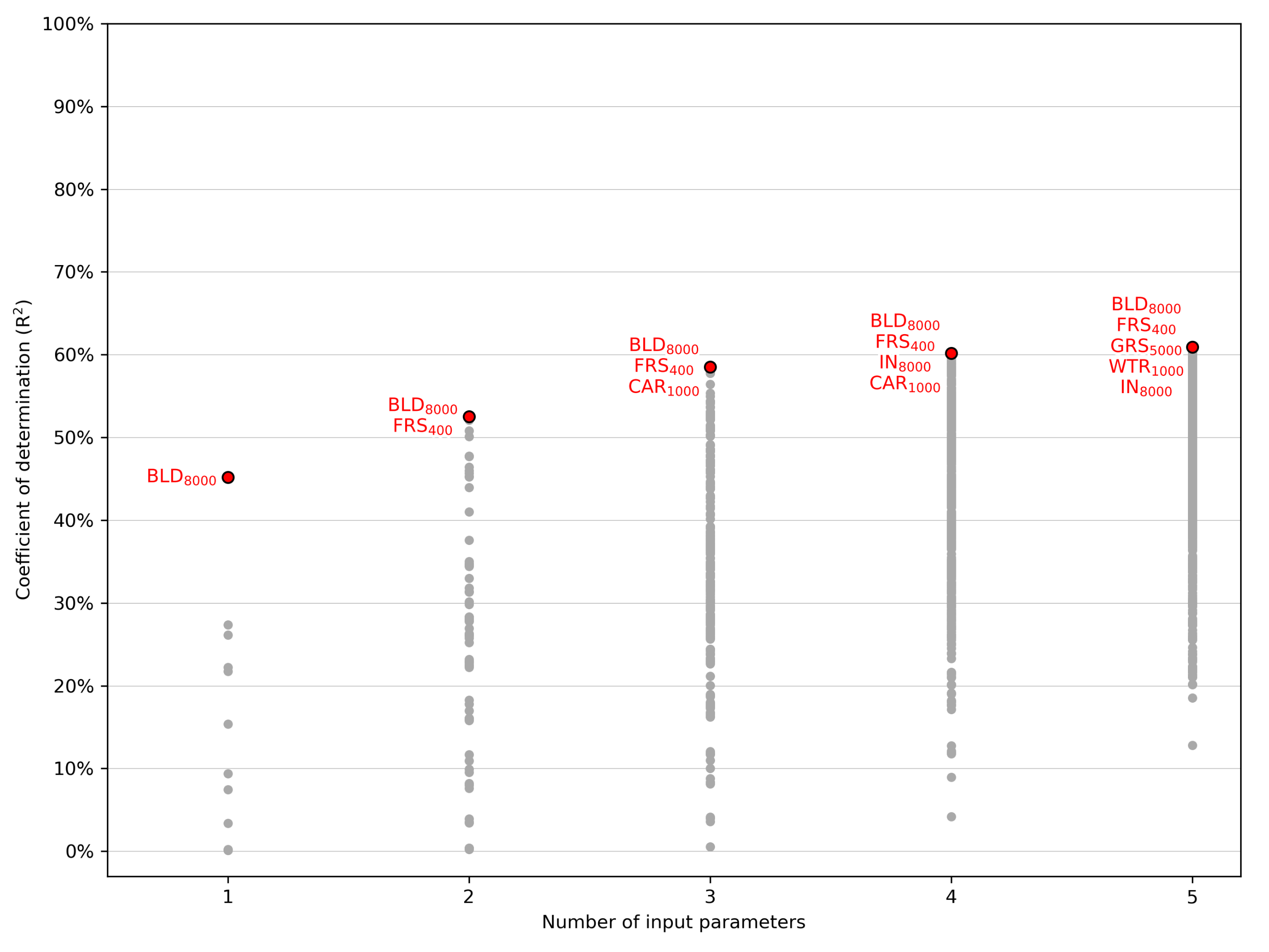
Two experiments with neural networks were conducted. All possible combinations of emission and land cover factors were tested, with the number of selected factors being 5 in the first experiment. A total of 1585 combinations were tested. In the following graph, each point represents the performance of neural network models. The most efficient models for each number of the input parameters are highlighted (Figure 12).
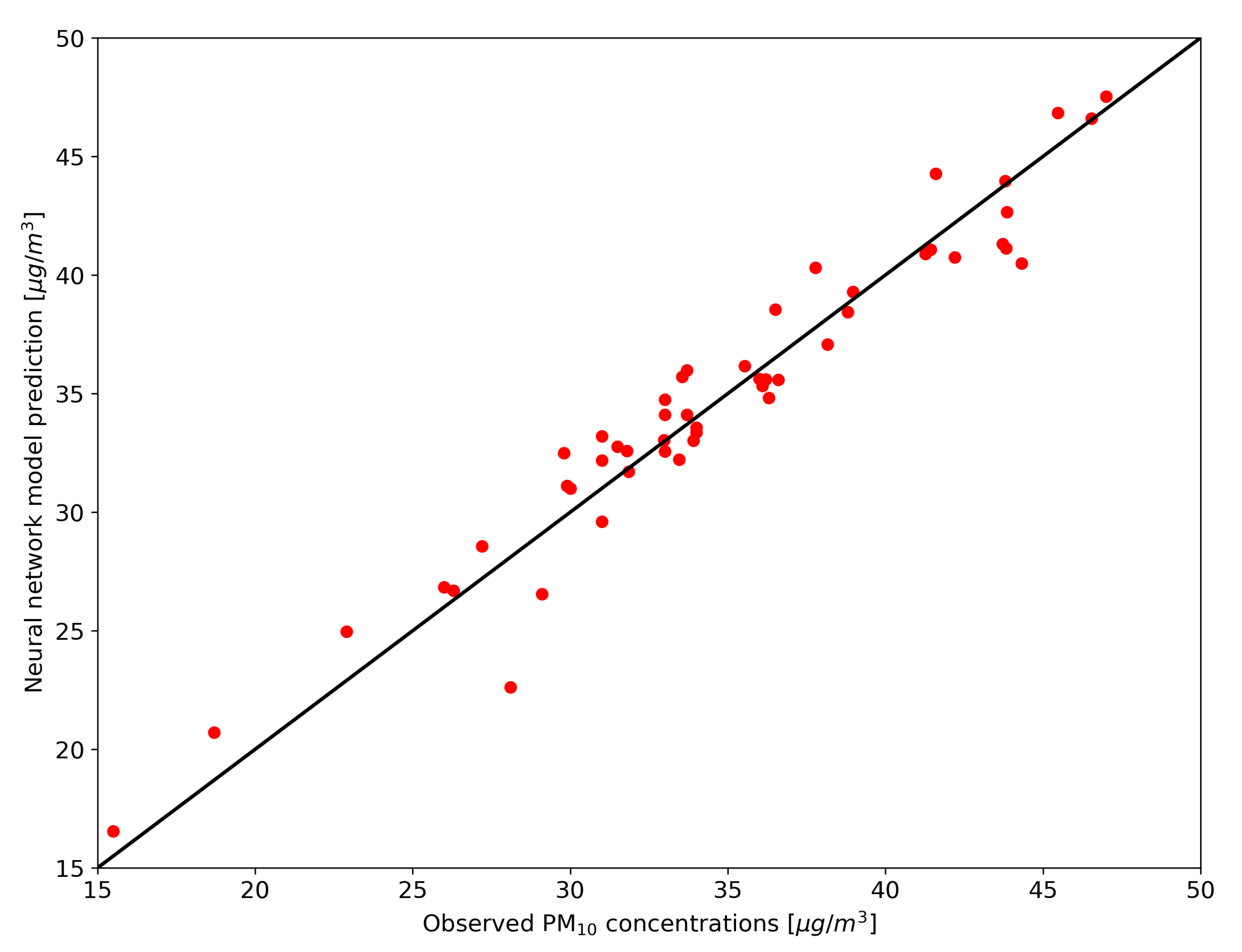
The best performing model was a neural network model containing the B L D 400 , B L D 8000 , G R S 5000 , I N 2000 and C A R 1000 factors. The R 2 of the model was 0.937 (Figure 13).
All possible input factor combinations with Gaussian model results and land cover factors were tested in the second experiment. The number of input factors was limited to five again. 381 combinations were tested. In the following graph, each point represents the performance of neural network models. The most efficient models for each number of the input parameters are highlighted (Figure 14).
The best performing model was a neural network model containing the B L D 400 , F R S 400 , G R S 5000 , M O D I N and M O D C A R factors. The R 2 of the model was 0.938 (Figure 15).
It was required to train 1501 neural networks for each tested combination of the input factors. It means that in total, approximately 2.95 million neural networks needed to be trained.

5. Discussion

Two sets of input data were selected for the LUR model construction; the first dataset consisted of emission factors and land cover factors, while the second dataset comprised Gaussian model results and land cover factors. The LUR model construction was performed via two techniques, the first one was standard linear regression, the second one was the multilayer perceptron neural network. A set of LUR models was created for different selections of input factors (≤5) in each of the four experiments, determined by the input dataset and model construction technique. The best model in each experiment was defined by the R 2 score of the result (Table 4).
A comparison of different possible model performance measures of all four best models is presented in Table 5.
Nearly all model performance measures indicate a better performance of neural network models. The only exception is the normalized mean bias, which shows the low overestimation or underestimation of neural network models, while linear regression models show almost zero values. This is the natural behaviour of linear models.
All the best models provide significantly improved results over the pure Gaussian model. The R 2 of the Gaussian model was 0.485, and its results compared to the measurements are shown in Figure 16. There are several monitoring stations where the Gaussian model significantly overestimated or underestimated the measured values. The values were overestimated at the monitoring sites in forested areas and underestimated in rural areas with a high percentage of open soil near the monitoring stations. This clearly shows the limitations of pure Gaussian models, which do not include the influence of land cover factors.
Both linear regression-based LUR models provided a similar performance, the R 2 of the models was 0.639 for the emission factor linear model and 0.652 for the linear model based on the Gaussian model results. The results of these LUR models are similar to those of the other LUR models, which are 0.65 in Bitta et al. [31], 0.58 in Liu et al. [49] or 0.66–0.76 in Masiol et al. [50]. A more detail comparison of these studies and the model of the study is not possible, since each model used a different set of variables, different time scales, etc. Gaussian model results were more accurate at the monitoring sites representing urban or industrial sites. The LUR model, which included land cover factors, provided better results in rural and natural environments.
Both neural network-based LUR models performed significantly better than their linear regression-based counterparts. Both models showed similar results with R 2 of 0.937 and 0.938. A better performance of neural network-based models is the expected result, since nonlinear regression provided by neural networks can better reflect a generally nonlinear nature of pollution dispersion.
One can also compare the performance of linear regression and neural network models with the same input data. This comparison is provided in the following two tables (Table 6 and Table 7).
It is clear that neural network models provide significantly more accurate results than linear regression models. Nonlinear regression provided by neural network models performed best with input factors that had slightly worse results in the linear regression model than the best possible linear regression model inputs. Conversely, inputs that provided the best linear regression model results slightly underperformed when they were used as inputs of the neural network model. There are factors that better reflect the nonlinear behaviour of air pollution dispersion.
Such high R 2 values can have several reasons. The selected method of the model construction may provide high quality results or be distorted due to overfitting (even though we tried to avoid it) or the monitoring station mesh dominated by urban background stations (42 out of 47 stations). Higher variability among monitoring stations would definitively bring higher confidence in the results.
For each LUR model construction technique, both input factor data sets provided a similar quality of results. The question arises whether Gaussian dispersion modelling is a necessary step. The Gaussian dispersion model in this case was highly computationally intensive. It took several processor years of processing, which could have been avoided. This hypothesis also requires further investigation on different datasets.
LUR models are empirical models that are constructed as statistical models based on the data provided. Each LUR model represents only a specific time and space interval, which is reflected in input data. The model formula and coefficients implicitly represent the effects of general phenomena that affect air pollution. Meteorological factors, which demonstrably influence pollution dispersion, such as precipitation, temperature, thermal stability, etc., are typical examples of factors that are implicitly reflected in LUR model coefficients. It also means that a different time period or different area of interest produces its own set of LUR model coefficients. The goal of LUR modelling should not be to provide one universally applicable model. The goal is to provide an algorithm that generates the LUR model fitting the best selected time period and area of interest.

6. Conclusions

We managed to significantly improve the performance of the standard linear regression-based LUR model by replacing the linear regression algorithm with the multilayer perceptron neural network. This is an innovative approach that has the potential of future improvement of LUR modelling. The modelling technique described in the study requires further investigation and development. The goal should be a standardized modelling algorithm and standardized input datasets that provide credible results for decision makers.

Author Contributions

Conceptualization, J.B. and V.S.; Data curation, J.B. and V.S.; Formal analysis, J.B., V.S. and A.S.K.; Methodology, J.B.; Supervision, J.B.; Validation, V.S. and A.S.K.; Writing—original draft, J.B. and V.S.; Writing—review & editing, V.S. and A.S.K. All authors have read and agreed to the published version of the manuscript.

Funding

The research was funded by the project solved in cooperation between the Czech Republic and JINR (3+3 project) “Development of novel techniques of air pollution distribution estimation”, 2020, No. 05-6-1118-2014/2023, main investigators: V. Svozilík, J. Bitta.

Institutional Review Board Statement

Not applicable.

Informed Consent Statement

Not applicable.

Data Availability Statement

Modelling data are available at https://bit.ly/3cAuMfi (accessed on 31 March 2021), for further info please contact authors.

Acknowledgments

Access to the computing and storage facilities owned by parties and projects contributing to the National Grid Infrastructure MetaCentrum under the programme “Projects of Large Research, Development, and Innovations Infrastructures” (CESNET LM2015042) is greatly appreciated. The research was supported in part by the “Govorun” computational cluster provided by the Laboratory of Information Technologies of the Joint Institute for Nuclear Research in Dubna, Moscow Region, Russia.

Conflicts of Interest

The authors declare no conflict of interest.

Abbreviations

The following abbreviations are used in this manuscript:
ADMOSSAnalytical Dispersion Modelling Supercomputer System
ANNArtificial Neural Network
APIApplication Programming Interface
CESNETCzech Education and Scientific NETwork
CUZKČeský úřad zeměměřický a katastrální/
Czech State Administration of Land Surveying and Cadastre
EEAEuropean Environment Agency
EUEuropean Union
GKUGeodetic and Cartographic Institute Bratislava
GUGiKMain Office of Geodesy and Cartography/Główny Urząd Geodezji i Kartografii
JINRJoint Institute for Nuclear Research
LURLand Use Regression
mMeter
MLPMulti-Layer Perceptron
PAHPolycyclic Aromatic Hydrocarbon
PM10Particulate Matter with a diameter of 10 microns
PM2.5Particulate Matter with a diameter of 2.5 microns
PMcoarseParticulate Matter Coarse
POPsPersistent Organic Pollutants
R2Coefficient of determination
SYMOSModelling System for Stationary Sources
VSB-TUOVSB—Technical University of Ostrava
ZABAGEDFeature Catalog ZABAGED®
ZBGISZákladná báza údajov pre geografický informačný systém/
Basic database for geographic information systems

Appendix A

Table A1. Annual concentration of PM10 in 2015 in the AIR TRITIA project area.
Annual Mean Concentration of PM10 in 2015
Monitoring StationLatitudeLongitudeConcentration
Bílý Kříž49.5026091718.5385608315.5
Čeladná49.5592155618.3483544422.9
Frýdek-Místek49.6717911118.3510702829.9
Návsí u Jablunkova49.5941944418.7439638928.1
Třinec-Kanada49.6723786118.6430377826.3
Třinec-Kosmos49.6681136118.6777991729.8
Český Těšín49.7489586118.6097258336.5
Havířov49.790977518.4068355636.2
Karviná49.8637961118.551452536.6
Orlová49.8756618.4336072236.1
Šunychl49.9275666718.3618469434.0
Věřňovice49.9246788918.422872541.6
Červená hora49.7771416717.5419463918.7
Opava-Kateřinky49.9449883317.9095305627.2
Ostrava-Fifejdy49.839187518.2636891733.9
Ostrava-Mariánské Hory49.8248597218.2636547231.5
Ostrava-Poruba/ČHMÚ49.8252944418.15927529.1
Ostrava-Přívoz49.8562583318.2697411136.3
Ostrava-Radvanice OZO49.8185386118.3403436133.7
Ostrava-Radvanice ZÚ49.8070563918.3391380642.2
Ostrava-Zábřeh49.7960394418.2471808331.8
Ostrava-Českobratrská49.8398518.28997533.7
Bielsko-Biała, ul. Kossak-Szczuckiej49.81346419.02731835.5
Cieszyn, ul. Mickiewicza49.73813618.63906933.0
Częstochowa, ul. Baczyńskiego50.83638919.13011131.9
Dąbrowa Górnicza, ul. Tysiąclecia50.32911119.23122241.4
Godów, ul. Gliniki49.92187518.47127844.3
Katowice, ul. Kossutha50.26461118.97502839.0
Katowice, ul. Plebiscytowa50.24679519.01946946.5
Knurów, ul. Jedności Narodowej50.23316718.65572243.8
Lubliniec, ul. Piaskowa50.65835718.6962238.2
Rybnik, ul. Borki50.11118118.51613947.0
Tarnowskie Góry, ul. Litewska50.44473618.82963937.8
Zabrze, ul. M. Curie-Skłodowskiej50.316518.77237543.9
Zawiercie, ul. M. Skłodowskiej-Curie50.4795419.4330138.8
Żory, Os. Gen. Władysława Sikorskiego50.02868118.69122241.3
Żywiec, ul. Kopernika49.67160219.23444643.8
Martin, Jesenského49.0669444418.9219444426.0
Ružomberok, Riadok49.0791666719.302531.0
Žilina, Obežná49.2119444418.7711111130.0
Głubczyce, ul. Kochanowskiego50.20094217.81645333.0
Kędzierzyn-Koźle, ul. B. Śmiałego50.34960818.23657531.0
Kluczbork, ul. Mickiewicza50.97218118.20757533.0
Nysa, ul. Rodziewiczówny50.45898917.33190634.0
Opole, os.im.Armii Krajowej50.67685617.95027831.0
Opole, ul. Minorytów50.66696117.92279733.0
Zdzieszowice, os. Piastów50.42353318.12073936.0

References

  1. Vallero, D.A. Fundamentals of Air Pollution, 5th ed.; Elsevier: Amsterdam, The Netherlands; Boston, MA, USA, 2014. [Google Scholar]
  2. Künzli, N.; Kaiser, R.; Medina, S.; Studnicka, M.; Chanel, O.; Filliger, P.; Herry, M.; Horak, F.; Puybonnieux-Texier, V.; Quénel, P.; et al. Public-health impact of outdoor and traffic-related air pollution: A European assessment. Lancet 2000, 356, 795–801. [Google Scholar] [CrossRef]
  3. Saxena, P. Air Pollution: Sources, Impacts and Controls; CAB International: Wallingford, Oxfordshire, UK; Boston, MA, USA, 2019. [Google Scholar]
  4. The Parliament of the EU; The Council of the EU. Directive 2008/50/EC of the European Parliament and of the Council of 21 May 2008 on ambient air quality and cleaner air for Europe. Off. J. Eur. Union 2008. Available online: https://eur-lex.europa.eu/legal-content/EN/TXT/HTML/?uri=CELEX:32008L0050 (accessed on 27 February 2021).
  5. United States Environmental Protection Agency (EPA US). OAQPS Guidline Series. Available online: https://nepis.epa.gov/Exe/ZyPDF.cgi/91005584.PDF?Dockey=91005584.PDF (accessed on 27 February 2021).
  6. Sutton, O.G. A Theory of Eddy Diffusion in the Atmosphere. Proc. R. Soc. A Math. Phys. Eng. Sci. 1932, 135, 143–165. [Google Scholar] [CrossRef]
  7. Bubník, J.; Keder, J.; Macoun, J.; Maňák, J.; Jareš, R.; Karel, J.; Smolová, E.; Hladík, M.; Janatová, L.; Škáchová, H.; et al. SYMOS’97—Systém Modelování Stacionárních Zdrojů, 1998 actualised 2014; Czech Hydrometeorological Institute: Prague, Czech Republic, 2014. [Google Scholar]
  8. Turner, D.B.; Schulze, R.H. Practical Guide to Atmospheric Dispersion Modeling, 1st ed.; Trinity Consultants: Pitsburgh, PA, USA, 2007. [Google Scholar]
  9. Atkinson, D.; Bailey, D.; Irwin, J.; Touma, J. Improvements to the EPA Industrial Source Complex Dispersion Model. J. Appl. Meteorol. 1997, 36, 1088–1095. [Google Scholar] [CrossRef]
  10. United States Environmental Protection Agency (EPA US). Analyses of the CALMET/CALPUFF Modeling System in a Screening Mode; EPA US: Washington, DC, USA, 1998.
  11. Benson, P.E. A review of the development and application of the CALINE3 and 4 models. Atmos. Environ. Part Urban Atmos. 1992, 26, 379–390. [Google Scholar] [CrossRef]
  12. United States Environmental Protection Agency (EPA US). AERMOD: Description of Model Formulation. Available online: https://nepis.epa.gov/Exe/ZyPDF.cgi/P1009OXW.PDF?Dockey=P1009OXW.PDF (accessed on 27 February 2021).
  13. Bubnik, J.; Keder, J.; Macoun, J. Metodika SYMOS’97—Metodika Výpočtu Znečištění Ovzduší u Bodových, Plošných Nebo Liniových Stacionárních Zdrojů; Czech Hydrometeorological Institute: Prague, Czech Republic, 1997. [Google Scholar]
  14. Buckland, A.; Middleton, D. Nomograms for calculating pollution within street canyons. Atmos. Environ. 1999, 33, 1017–1036. [Google Scholar] [CrossRef]
  15. ATEM. Imisní Model ATEM. Available online: http://www.atem.cz/soubory/ke_stazeni/IMATEM_metodika.pdf (accessed on 31 March 2021).
  16. Hoek, G.; Beelen, R.; de Hoogh, K.; Vienneau, D.; Gulliver, J.; Fischer, P.; Briggs, D. A review of land-use regression models to assess spatial variation of outdoor air pollution. Atmos. Environ. 2008, 42, 7561–7578. [Google Scholar] [CrossRef]
  17. Gilbert, N.; Goldberg, M.; Beckerman, B.; Brook, J.; Jerrett, M. Assessing spatial variability of ambient nitrogen dioxide in Montréal, Canada, with a land-use regression model. J. Air Waste Manag. Assoc. 2005, 55, 1059–1063. [Google Scholar] [CrossRef] [PubMed] [Green Version]
  18. Briggs, D. The role of GIS: Coping with space (and time) in air pollution exposure assessment. J. Toxicol. Environ. Health Part A 2005, 68, 1243–1261. [Google Scholar] [CrossRef] [PubMed]
  19. Hendl, J. Prehled Statistickych Metod Zpracovani Dat: Analyza a Metanalyza Dat; Portal: Prague, Czech Republic, 2006. [Google Scholar]
  20. Gelman, A. Data Analysis Using Regression and Multilevel/Hierarchical Models; Cambridge University Press: Cambridge, UK, 2007. [Google Scholar]
  21. Van den Bossche, J.; De Baets, B.; Verwaeren, J.; Botteldooren, D.; Theunis, J. Development and evaluation of land use regression models for black carbon based on bicycle and pedestrian measurements in the urban environment. Environ. Model. Softw. 2018, 99, 58–69. [Google Scholar] [CrossRef] [Green Version]
  22. Lee, J.H.; Wu, C.F.; Hoek, G.; de Hoogh, K.; Beelen, R.; Brunekreef, B.; Chan, C.C. LUR models for particulate matters in the Taipei metropolis with high densities of roads and strong activities of industry, commerce and construction. Sci. Total. Environ. 2015, 514, 178–184. [Google Scholar] [CrossRef] [PubMed]
  23. Hsu, C.Y.; Wu, C.D.; Hsiao, Y.P.; Chen, Y.C.; Chen, M.J.; Lung, S.C. Developing Land-Use Regression Models to Estimate PM2.5-Bound Compound Concentrations. Remote Sens. 2018, 10, 1971. [Google Scholar] [CrossRef] [Green Version]
  24. Wu, C.D.; Chen, Y.C.; Pan, W.C.; Zeng, Y.T.; Chen, M.J.; Guo, Y.L.; Lung, S.C.C. Land-use regression with long-term satellite-based greenness index and culture-specific sources to model PM2.5 spatial-temporal variability. Environ. Pollut. 2017, 224, 148–157. [Google Scholar] [CrossRef] [PubMed]
  25. McLachlan, G.J.; Do, K.A.; Ambroise, C. Analyzing Microarray Gene Expression Data; John Wiley and Sons: Hoboken, NJ, USA, 2004. [Google Scholar]
  26. Bitta, J. Systém Pro Hodnocení Stavu Životního Prostředí Pomocí Matematického Modelování Pro Oblasti Zatížené Metalurgickým Průmyslem. Ph.D. Thesis, VSB—Technical University of Ostrava, Ostrava, Czech Republic, 2011. [Google Scholar]
  27. Zákon, č. 201/2012 Sb. O ochraně ovzduší [Clean Air Act]; Parliament of the Czech Republic: Prague, Czech Republic, 2012. [Google Scholar]
  28. Jančík, P. Atlas Ostravského Ovzduší, 1st ed.; VŠB-TU: Ostrava, Czech Republic, 2013. [Google Scholar]
  29. Jančík, P.; Pavlíková, I.; Hladký, D.; Michalík, J.; Svozilík, V. Air Progres Czecho-Slovakia. Available online: http://apcs.vsb.cz/data/Studie-APCS.pdf (accessed on 7 September 2019).
  30. Ďurčanská, D.E.A. Riadenie Kvality Ovzdušia [Air Quality Management], 1st ed.; Žilinská Univerzita V Žiline—EDIS—Vydavate’ské Centrum ŽU: Žilina, Slovakia, 2020. [Google Scholar]
  31. Bitta, J.; Pavlikova, I.; Svozilik, V.; Jancik, P. Air Pollution Dispersion Modelling Using Spatial Analyses. ISPRS Int. J. Geo-Inf. 2018, 7, 489. [Google Scholar] [CrossRef] [Green Version]
  32. Hastie, T.; Tibshirani, R.; Friedman, J. The Elements of Statistical Learning: Data Mining, Inference and Prediction; Springer: New York, NY, USA, 2009. [Google Scholar]
  33. Lautenschlager, F.; Becker, M.; Kobs, K.; Steininger, M.; Davidson, P.; Krause, A.; Hotho, A. OpenLUR: Off-the-shelf air pollution modeling with open features and machine learning. Atmos. Environ. 2020, 233, 117535. [Google Scholar] [CrossRef]
  34. Alam, M.S.; McNabola, A. Exploring the modeling of spatiotemporal variations in ambient air pollution within the land use regression framework: Estimation of PM10 concentrations on a daily basis. J. Air Waste Manag. Assoc. 2015, 65, 628–640. [Google Scholar] [CrossRef] [PubMed]
  35. Air Tritia. Available online: https://www.interreg-central.eu/Content.Node/AIR-TRITIA.html (accessed on 1 November 2020).
  36. European Environment Agency. Air Quality in Europe: 2015 Report; Publications Office of the European Union: Luxembourg, 2015. [Google Scholar] [CrossRef]
  37. European Environment Agency. Annual Mean PM10 Concentrations in 2015. Available online: https://www.eea.europa.eu/data-and-maps/figures/annual-mean-pm10-concentrations-in (accessed on 1 November 2020).
  38. Macoun, J.e.a. Air Pollution and Atmospheric Deposition in Data, the Czech Republic, 2015; Czech Hydrometeorological Institute: Prague, Czech Republic, 2016. [Google Scholar]
  39. Sadowski, T.E.A. Stan Srodowiska w Wojewodztwie Slaskim w 2015 Roku; PIOS Katowice: Katowice, Poland, 2016. [Google Scholar]
  40. Gaworski, K.E.A. Wyniki Pomiarow Uzyskanych w 2015 Roku na Stacjach Jakosci Powietrza w Wojewodztwie Opolskim; PIOS Opole: Opole, Poland, 2016. [Google Scholar]
  41. Tritia, A. Air Quality Management System. Available online: https://aqms.vsb.cz/ (accessed on 27 February 2021).
  42. Modeling System for Stationary Resources (SYMOS’97). Czech Hydrometeorological Institute: Prague. Available online: https://www.idea-envi.cz/symos-97-en.html (accessed on 27 February 2021).
  43. CUZK. ZABAGED. Available online: https://geoportal.cuzk.cz/(S(dlueg0h03ufdmtu4thyb1a5f))/default.aspx?lng=EN&mode=TextMeta&text=dSady_zabaged&side=zabaged&menu=24 (accessed on 1 November 2020).
  44. GUGiK. Baza Danych Obiektów Topograficznych (BDOT). Available online: https://www.geoportal.gov.pl/dane/baza-danych-obiektow-topograficznych-bdot (accessed on 1 November 2020).
  45. GKU. ZBGIS. Available online: https://www.geoportal.sk/sk/zbgis/ (accessed on 1 November 2020).
  46. Anaconda. Anaconda. Available online: https://www.anaconda.com (accessed on 1 November 2020).
  47. CESNET. Metacentrum NGI. Available online: https://www.metacentrum.cz/en/index.html (accessed on 1 November 2020).
  48. JINR. Govorun Supercomputer. Available online: http://hlit.jinr.ru/en/about_govorun_eng/ (accessed on 1 November 2020).
  49. Liu, W. Land use regression models coupled with meteorology to model spatial and temporal variability of NO2 and PM10 in Changsha, China. Atmos. Environ. 2015, 116, 272–280. [Google Scholar] [CrossRef]
  50. Masiol, M.; Zíková, N.; Chalupa, D.; Rich, D.; Ferro, A.; Hopke, P. Hourly land-use regression models based on low-cost PM monitor data. Environ. Res. 2018, 167, 7–14. [Google Scholar] [CrossRef] [PubMed]
Figure 1. Wind direction probability distribution, Basemap: OpenStreetMap (CC BY-SA 4.0).
Atmosphere 12 00452 g001
Figure 2. Under- and overfitting of the prediction model.
Atmosphere 12 00452 g002
Figure 3. Tritia region and pollution monitoring sites, Basemap: OpenStreetMap (CC BY-SA 4.0).
Atmosphere 12 00452 g003
Figure 4. Annual average PM10 concentrations in the EU, 2015 (European Environment Agency (EEA)) [37].
Atmosphere 12 00452 g004
Figure 5. PM10 emission distribution in the area of interest, Basemap: OpenStreetMap (CC BY-SA 4.0).
Atmosphere 12 00452 g005
Figure 6. Flowchart of the modelling experiment.
Atmosphere 12 00452 g006
Figure 7. Spearman’s correlations of the built-up land cover factor with PM10 concentrations.
Atmosphere 12 00452 g007
Figure 8. Performance comparison of linear models with emission + land cover factors.
Atmosphere 12 00452 g008
Figure 9. Observed PM10 concentrations vs. best model predictions.
Atmosphere 12 00452 g009
Figure 10. Performance comparison of linear models with Gaussian model results + land cover factors.
Atmosphere 12 00452 g010
Figure 11. Observed PM10 concentrations vs. best model predictions.
Atmosphere 12 00452 g011
Figure 12. Performance comparison of neural network models with emission + land cover factors.
Atmosphere 12 00452 g012
Figure 13. Observed PM10 concentrations vs. best model predictions.
Atmosphere 12 00452 g013
Figure 14. Performance comparison of neural network models with Gaussian model results + land cover factors.
Atmosphere 12 00452 g014
Figure 15. Observed PM10 concentrations vs. best model predictions.
Atmosphere 12 00452 g015
Figure 16. Observed PM10 concentrations vs. Gaussian model results.
Atmosphere 12 00452 g016
Table 1. Considered regression factors.
Factor GroupFactorCodeUnit
Emission factorsIndustrial sourcesINt/y
Car trafficCARt/y
Domestic heatingDHt/y
Land cover factorsGrass coveredGRS%
Built-inBLD%
ForestedFRS%
Open soilSOIL%
Water bodiesWTR%
Gaussian model resultsPollution from industrial sourcesMOD I N μg/m3-
Pollution from domestic heatingMOD D H μg/m3
Pollution from car trafficMOD C A R μg/m3
Table 2. Emission of PM10 in the area of interest.
CountryPollution SourcesNo. of SourcesEmission [t/y]
CzechiaIndustrial sources47281325
Domestic heating52,6691225
Car traffic59,651514
PolandIndustrial sources17,4859962
Domestic heating131,74120,603
Car traffic403,4511965
SlovakiaIndustrial sources1366233
Domestic heating33,5762686
Car traffic34,009301
Total738,67638,814
Table 3. Selected factors.
Factor GroupFactorCodeUnitPerimeter(s) [m]
Emission factorsIndustrial sourcesINt/y2000/8000
Car trafficCARt/y1000/10,000
Domestic heatingDHt/y1000/5000
Land cover factorsGrass coveredGRS%5000
Built-inBLD%400/8000
ForestedFRS%400
Open soilSOIL%5000
Water bodiesWTR%1000
Gaussian model resultsPollution from industrial sourcesMOD I N μg/m3-
Pollution from domestic heatingMOD D H μg/m3-
Pollution from car trafficMOD C A R μg/m3-
Table 4. R 2 values of the best models.
Emission + Land Cover FactorsGaussian Model + Land Cover Factors
Linear regression model0.6390.652
Neural network model0.9370.938
Table 5. Model performance measures.
Model Performance MeasureEmission + Land Cover FactorsEmission + Land Cover FactorsGaussian Model + Land Cover FactorsGaussian Model + Land Cover Factors
Linear Regression ModelNeural Network ModelLinear Regression ModelNeural Network Model
Correlation0.8070.9680.8240.968
R20.6390.9370.6520.938
Normalized mean bias2.5 * 10−160.001454 * 10−16−0.00172
Normalized root mean square error0.11430.0483220.10980.048258
Table 6. R 2 values of the best linear regression models and neural network models with the same inputs.
Emission + Land Cover FactorsGaussian Model + land Cover Factors
Linear regression model0.6390.652
Neural network model0.8540.810
Table 7. R 2 values of the best neural network models and linear regression models with the same inputs.
Emission + Land Cover FactorsGaussian Model + Land Cover Factors
Linear regression model0.5160.564
Neural network model0.9370.938
Publisher’s Note: MDPI stays neutral with regard to jurisdictional claims in published maps and institutional affiliations.