Article

Application of Morrison Cloud Microphysics Scheme in GRAPES_Meso Model and the Sensitivity Study on CCN’s Impacts on Cloud Radiation

1
Key Laboratory of Meteorological Disaster, Ministry of Education/Joint International Research Laboratory of Climate and Environment Change/Collaborative Innovation Center on Forecast and Evaluation of Meteorological Disasters, Nanjing University of Information Science and Technology, Nanjing 210044, China
2
Chinese Academy of Meteorological Sciences (CAMS), State Key Laboratory of Severe Weather (LASW), China Meteorological Administration (CMA), Beijing 100081, China
3
Southern Marine Science and Engineering Guangdong Laboratory (Zhuhai), Sun Yat-sen University, Zhuhai 519082, China
4
Key Laboratory of South China Sea Meteorological Disaster Prevention and Mitigation of Hainan Province, Hainan Meteorological Administration, Haikou 570203, China
5
Beijing Meteorological Service Center, China Meteorological Administration (CMA), Beijing 100089, China
*
Authors to whom correspondence should be addressed.
Atmosphere 2021, 12(4), 489; https://doi.org/10.3390/atmos12040489
Submission received: 10 March 2021 / Revised: 2 April 2021 / Accepted: 8 April 2021 / Published: 13 April 2021
(This article belongs to the Section Atmospheric Techniques, Instruments, and Modeling)

Abstract

:
In the present study, the Morrison double-moment cloud microphysics scheme including mass and droplet number concentration of water and ice clouds is implemented into the Chinese mesoscale version of the Global/Regional Assimilation and Prediction System (GRAPES_Meso). Sensitivity experiments of different cloud condensation nuclei (CCN) values are conducted to study the impacts of CCN on cloud microphysical processes and radiation processes in East China. The model evaluation shows that the simulated cloud liquid water path (CLWP) is consistent with that of the National Center for Environment Prediction (NCEP) reanalysis, and the cloud optical depth (COD) and effective radius of cloud water (Rc) are in agreement with those of the Moderate Resolution Imaging Spectroradiometer (MODIS) datasets both in regional distribution and magnitudes. These comparisons illustrate the effectiveness of the Morrison scheme for the cloud processes in East China. For the study period of 8 to 12 October 2017, the sensitivity experiments show that with initial CCN number concentration (CCN0) increasing from 10 to 3000 cm−3, the maximum value of daily average Rc decreases by about 63%, which leads to a decrease of cloud-rain conversion rate. Moreover, the maximum value of daily average mixing ratio of cloud water (qc) increases by 133%, the maximum value of daily average mixing ratio of rain (qr) decreases by 44%, and the maximum value of daily average CLWP and COD increase by 100% and 150%, respectively. This results in about 65% increasing of the maximum value of daily average cloud downward shortwave radiative forcing (CDSRF) when CCN0 increases from 10 cm−3 to 3000 cm−3. The study indicates the important impacts of CCN on cloud properties and radiation effects.

1. Introduction

Clouds are an essential component for the earth’s water cycle, and intensely influence energy exchange between earth and atmosphere [1,2]. The interaction between clouds and aerosols directly affects cloud properties and microphysical processes by radiation and heat transfer, which then has important influences on weather and climate change. A reasonable cloud microphysics scheme describing the cloud micro and macro properties, formation, and evolution accurately are vital for the weather and climate model [3,4].
Cloud microphysics parameterization schemes are generally divided into bin schemes [5,6] and bulk schemes [7,8]. Bin schemes explicitly calculate the evolution of the particle size distribution and divide a hydrometeor size distribution into several size bins, based on the microphysical properties of hydrometeors and aerosol such as phase state, particle size, shape, density, which is widely used to study the liquid and ice-phase cloud microphysical processes [9,10]. Bulk schemes, therefore, become a feasible alternative for many applications. Bulk schemes can be further classified into single-moment and double-moment schemes. Single-moment schemes simulate only the mass mixing ratio of hydrometeors [11,12,13]. Double-moment schemes simulate both mass mixing ratio and number concentration of hydrometeors [14]. Double-moment microphysics schemes were widely used in the convective and layer clouds and precipitation [15,16]. Ferrier proposed a double-moment ice-phase volumetric water microphysics scheme to simulate the distribution of condensate in convective precipitation and layered cloud precipitation under different large-scale environmental conditions [17]. A relatively complete double-moment microphysics scheme was proposed to study cumulonimbus related issues, which can numerically calculate the number concentration of cloud (nc), raindrops (nr), ice (ni), snow (ns), and graupel (ng) droplets [18]. Double-moment schemes incorporate the number concentration of hydrometeors and increase the degrees of freedom of the particle size distribution, and the number and quality of hydrometeor particles in the physical mechanism are more coordinated, which is incorporated in climate or weather models and widely used in weather and climate simulations [19,20,21].
Morrison developed a double-moment microphysics scheme including five types of hydrometeors: cloud droplets, raindrops, ice, snow, and graupel [22]. The scheme considers a more elaborate and comprehensive microphysical process, mass concentration, and numerical concentration of the aquatic matter and is used to test real cases and ideal case studies [23,24,25,26]. The scheme is widely applied to investigate the influence of aerosol spectrum changes on the precipitation weather process. Therefore, this double-moment scheme has been widely used in the popular mesoscale models such as the NCAR/Penn fifth-generation Mesoscale Model (MM5) and the Weather Research and Forecasting (WRF) model. The Morrison scheme is implemented into the aerosol-climate model BCC_AGCM2.0.1_CUACE/Aero to evaluate model results for aerosols cloud properties and meteorological fields, the new model simulated a more realistic aerosol mass concentrations and optical depth compared with the original version [21]. The forecast of cold precipitation amount includes cloud ice mixing ratio, snow mixing ratio, and haze mixing ratio; the Morrison scheme can also forecast the number concentration [27]. Besides, the predicted particle properties (P3) scheme has been developed, and the scheme represents ice microphysics by emphasizing the pre-diction of particle properties rather than the separation of ice into different predefined categories [28]. Thompson had also developed a new bulk microphysical parameterization (BMP) to analyze the impact of cloud properties on radiation, precipitation amount and type, and aircraft icing, which has been updated to incorporate aerosols explicitly in a simple and cost-effective manner [29,30]. A comparative study of different microphysical schemes (Lin, WSM6, GCE, Thompson and Morrison) was carried out, and it was found that although the Thompson scheme and Morrison scheme set the cloud droplet concentration as a constant, the cloud droplet number concentration and cloud droplet spectrum of these two schemes are closer to the observation [31,32,33].
Cloud condensation nuclei (CCN) plays a crucial role in the double moment cloud microphysical processes. The CCN may influence the precipitation efficiency by determining the concentration and original particle size of the cloud droplet. Studies show that the increase of CCN will lead to an increase in the concentration of cloud droplets and a decrease in the size of cloud droplet particles, which then suppresses warm cloud precipitation [34,35]. Besides, with the increase of CCN, the mixing ratio of cloud water (qc) in the condensate increases, the size of droplets decreases, and raindrops decrease, accordingly [36]. CCN can also affect the cloud radiative forcing through the indirect effect [37]. That is, the increase of CCN will lead to more and smaller cloud droplets, which then generates more cloud reflection. The effective radius of cloud water (Rc) is an important cloud physical characteristic parameter, and it can affect the scattering characteristics of clouds. For a given liquid water content or ice water content, cloud with smaller Rc or the effective radius of cloud ice (Ri) will reflect/scatter more solar radiation [38]. The distribution of the cloud optical depth (COD) is affected by cloud volume, cloud water content, and Rc. The area with large cloud volume is basically the large value area of COD. From the perspective of vertical change, the change of COD is greatly affected by the change of liquid water content with height [39].
These studies on CCN are mainly concentrated in areas where aerosol pollution is relatively light, while for the heavily polluted North China Plain, research about the impact of CCN on cloud microphysical processes is still poor. In this study, the Morrison double-moment cloud microphysics scheme is implemented into the GRAEPS_Meso model. The evaluation of the simulation results and the impacts of different CCN on microphysical quantities and cloud radiation forcing have been presented. Table 1 shows the related acronyms of cloud microphysical characteristics used in this paper, such as CCN, Rc, Ri, and so on. The study indicates the impacts of CCN on cloud properties and radiation effects are important. There is high pollution in East China, and the number concentration of CCN changes drastically. The results of my study are very important for the improvement of forecasting ability and the model performance in East China.

2. Model and Scheme

2.1. GRAPES_Meso

The mesoscale version of the new-generation Global/Regional Assimilation and Prediction System (GRAPES_Meso) is an operational weather forecasting model developed by the Chinese Academy of Meteorological Sciences, which mainly consists of 3-D meteorological field data assimilation, the full compressible dynamic framework, and a physical parameterization package [40,41,42]. This model is generally used for operational forecasting and scientific research about the medium- and short-term weather conditions in China [43,44]. It has also been widely used for the study of cloud, aerosol, and the interaction between cloud and aerosol in China for about 20 years [45,46]. The application results of the GRAPES_Meso model in national and regional areas are satisfactory [47,48]. The model adopts a height-based terrain-following coordinate, a semi-implicit and semi-Lagrangian temporal advection scheme for time integration discretization, an Arakawa-C staggered grid format, a central finite-difference scheme for horizontal discretization, and a non-hydrostatic approximation scheme for vertical discretization [49]. The physical parameterization schemes selected in this study include Rapid Radiative Transfer Model (RRTM) longwave radiation scheme [50], Goddard shortwave radiation scheme [51], the Monin–Obukhov surface layer scheme [52], the Noah land surface model [53], the Betts–Miller–Janjic (BMJ) cumulus convection scheme [54], and the Medium-Range Forecast (MRF) boundary layer scheme [55].

2.2. Morrison Cloud Microphysical Scheme

Morrison double-moment microphysics scheme including mass mixing ration of and number concentration predictions of hydrometeors particles is integrated into GRAPES_Meso to simulate the cloud process in East Asia in this study [56]. The governing equations of the Morrison scheme for the mass mixing ratio and number concentration of hydrometeors are as follows [57,58]:
q t = ( v q ) + z ( V q x ) + D q + q t PRO + q t COND / DEP + q t AUTO + q t COAG + q t MLT / FRZ + q t MULT
N t = v N + z V N x + D N + N t PRO + N t EVAP / SUB + N t AUTO + N t SELF + N t COAG + N t MLT / FRZ + N t MULT
where q and N represent the mass mixing ratio and number concentration of all hydrometeors; they depend on space variables x, y, and z and time, t. v is the three-dimensional wind vector. VNx and Vqx are number- and mass-weighted the final falling velocity of each particle. ∇D is a turbulent diffusion operator for models that parameterize turbulent mixing. The first three terms on the right-hand side of Equations (1) and (2) represent the advection, sedimentation, and the turbulent diffusion term of qx and Nx, respectively, and they are calculated by dynamic frame in the GRAPES_Meso model. Table 2 summarized all the transformation processes in Equations (1) and (2) [22].
The Morrison scheme includes not only the double-moment of warm cloud processes but also the double-moment of cold cloud processes. It can predict water cloud mass mixing ration, number concentration (qc, mixing ratio of rainwater (qr), nc, nr), cloud mass mixing ratio, and number concentration (mixing ratio of ice (qi), qg, mixing ratio of snow (qs), ni, ng, ns). The scheme includes 19 microphysics processes mass mixing ratio related to mass mixing ratio and 22 microphysics processes related to number concentration, respectively. The scheme uses the activation calculation method to calculate CCN, while this study uses logarithmic aerosol particle size distribution to drive the CCN spectrum. Therefore, it needs to preset an initial CCN number concentration (CCN0) as the assumed atmosphere condition [59]. The default setting of CCN0 is 250 cm−3, representing the typical continent cloud, and many studies use this fixed default values in the simulation due to the lack of aerosols activation scheme in most numerical weather prediction models and cloud simulation studies, which is one of the major reasons leading to model uncertainties from clouds features and processes.

2.3. Experiments Design
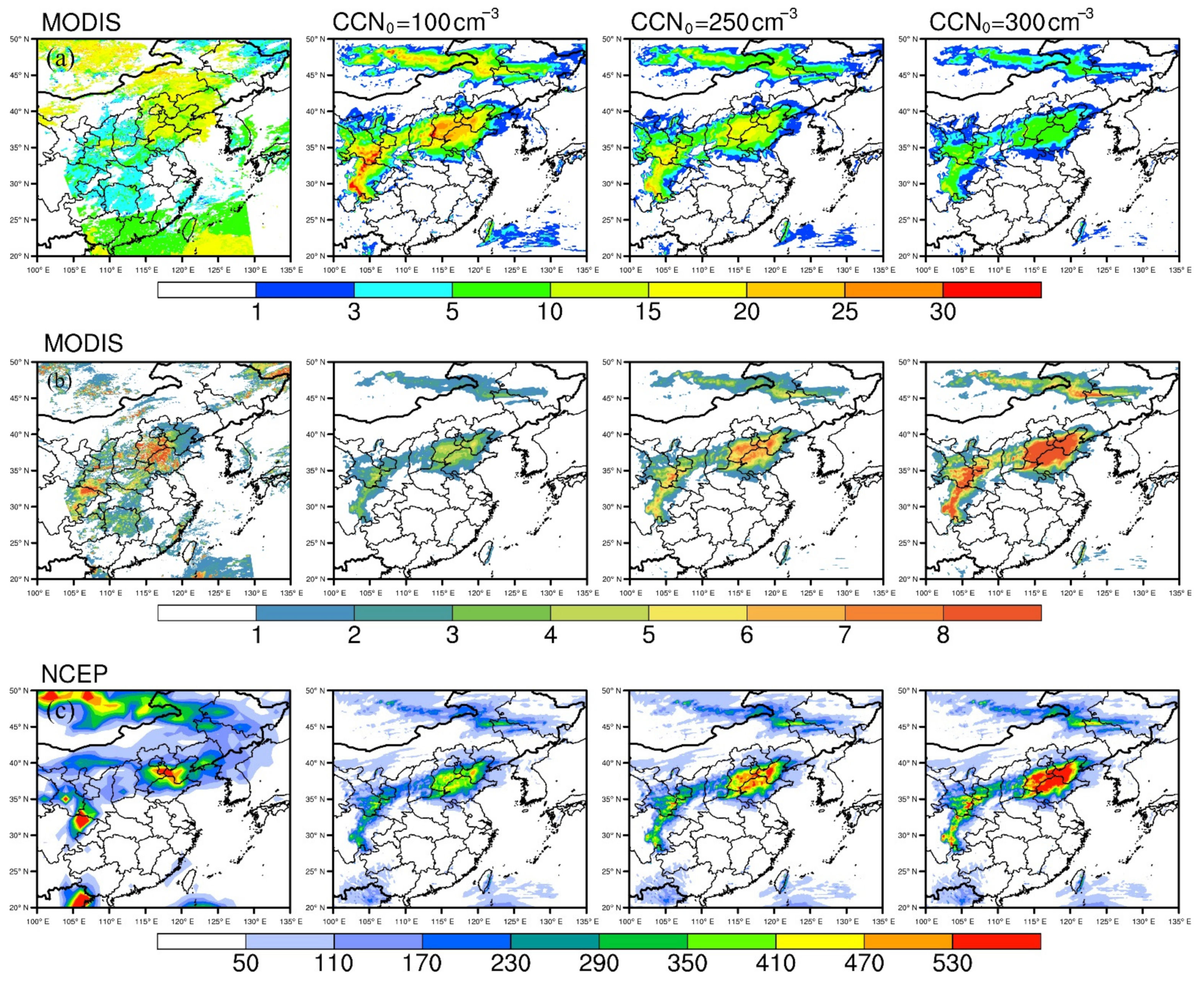
October is fall in China, and the frontal cloud system featured by stable stratus is the typical cloud system in this region. There are two frontal cloud systems passed through the study region in October. One occurred 8–12, another occurred 23–28; they are both frontal cloud systems dominated by stable stratus instead of convective clouds moved from northwest to southeast in East China, and the convective cloud is extremely weak during the cloud processes. The observation studies showed that the CCN varies largely in different regions and atmosphere conditions closely related to atmosphere critical supersaturation, aerosol loading, and species. It was reported that CCN could reach up to 1000 and 40,000 cm−3 in different conditions [60,61]. In North China, when the heaviest aerosol pollution occurs, the maximum value of CCN can get to 8000 cm3, and when the pollution is light, the minimum value of CCN can get to 8.2 cm−3 [62,63]. However, the initial values are usually set as fixed 250 cm−3 in the microphysics scheme in weather and climate models, which will lead to uncertainties in cloud radiation processes and then the model performance [36,64]. This study incorporates the Morrison scheme with the GRAPES_Meso model and sets the initial CCN as 250 cm3 to evaluate its applicability in the cloud system simulation in east Asia. The cloud liquid water path (CLWP) of reanalysis from the National Center for Environment Prediction (NCEP), COD and Rc of level-2 products from the Moderate Resolution Imaging Spectrometer (MODIS) are used for the model evaluation. Based on this, a set of sensitivity experiments CCN0 are set as 10, 100, 250, 600, 1000, 3000, 8000, and 10,000 cm−3 to study the effects of CCN on the cloud properties and radiation processes. The increase of CCN will lead to an increase in cloud droplets, which has been fully proved, so CCN and cloud droplets are in common to a certain degree, especially in variations. In this paper, we apply the Morrison double-moment scheme in the GRAPES model. However, in the current model, the processes of CCN activation have not been realized. We just set a wide range of possible CCN values directly (named as CCN0) to study the impacts of possible CCN’s changing on clouds radiation. Similar experiments have been conducted in previous studies [65,66]. Our following paper will focus on the different CCN activation schemes and its impacts on clouds radiation. For the model configuration, the initial input and lateral boundary are provided by NCEP final analysis (FNL) data (https://rda.ucar.edu/datasets/ (accessed on 20 July 2019)), with 0.25° × 0.25° horizontal grids and 6 h interval. The model domain covers east China, and its downwind area (20°–50° N, 100°–135° E). The model has 31 vertical layers from the surface to about 30 km. The model starting time is 00 UTC 8 October 2017, and its ending time is 00 UTC 13 October 2017, and the study period is from 00 UTC 8 to 12 October.

3. Model Evaluation

The CCN0 in Morrison scheme is assumed as the background of continent atmospheric condition 250 cm−3 in the model evaluation; in contrast, CCN of 100 and 300 cm−3 are also used for comparison in this section. Compared with WDM6 scheme in GRAPES_Meso, Morrison scheme has better performance in simulating the cloud microphysical characteristics in this study (Figures S1–S3). The correlation coefficient (CORR) and Root Mean Squared Error (RMSE) of CLWP, Rc, and COD between observations and simulations of Morrison and WDM6 schemes with setting CCN values as 250 cm−3 are calculated in the supplementary material (Table S1); it also can be seen that the simulations of Morrison scheme are better than those of WDM6 scheme.
Figure 1a shows the modeled average Rc, COD, and CLWP (CCN set as 100, 250, and 300 cm−3) from 8 to 12 October 2017 and cloud MODIS Rc, COD, and CLWP of NCEP Analysis. The comparison of modeled Rc with that of MODIS shows that there are obvious differences among the modeled Rc when the CCN is set as 100, 250, and 300 cm−3, indicating the great impacts of CCN on clouds particle size. In general, modeled Rc is the most consistent with the MODIS Rc when CCN is 250 cm−3 while Rc is generally bigger when CCN is 100 cm−3 and smaller when CCN is 300 cm−3 than those of MODIS. This is because more CCN means more cloud particles sharing the same cloud water and the reduction of the particles’ size. The size reduction of cloud particles with the CCN increasing causes the decreasing of the auto transformation process from clouds to rain, which further results in more cloud water in the atmosphere, so modeled COD and CLWP are both increased with the CCN decreasing from 100, 250 to 300 cm−3 (Figure 1b,c). Corresponding to the Rc varying, modeled COD and CLWP change distinctly when CCN increases from 100, 250 to 300 cm−3, suggesting the possible impacts of CCN on cloud radiation by Rc, COD, and CLWP. Moreover, the two parameters agree the best with those between MODIS COD and NCEP CLWP when CCN is 250 cm−3, illustrating the basic rationality of 250 cm−3 when CCN has to be set as a constant when aerosols activation scheme and aerosols processes are absent in the numerical weather prediction (NWP) models. We also compare the results between model and observed data by using the case from 23 to 28 October 2017 (Figures S4–S6). When the initial CCN is set as 250 cm−3, simulations of Rc, COD and CLWP agree with those of MODIS and NCEP in space and time. CORR and RMSE of CLWP, Rc, and COD between observations and simulations with setting CCN values as 250 cm−3 are calculated in Table 3. In the case from 8 to 12 October 2017, the CORRs of the observed and simulated RC, COD, and CLWP are 0.54, 0.55, and 0.57, and the RMSEs are 8.9, 1.6, and 160.4. As for another case from 23 to 28 October 2017, the CORRs are 0.51, 0.48, and 0.55, and the RMSEs are 10.2, −2.1, and 173.8. All of CORRs have exceeded 0.05 significance level. These results show that the simulations when the initial CCN is set as 250 cm−3 agree with the observed data and are more accurate than those when setting CCN as 100 cm−3 or 300 cm−3. However, it is noteworthy that there are certain diversities between modeled Rc, COD, and CLWP even CCN is 250 cm−3 and those of MODIS and NCEP. The truth of the obvious differences between Rc, COD, and CLWP among the three experiments when CCN is 100, 250 or 300 cm3 indicates the important impacts of CCN on cloud key parameters. The CCN is set as the constant of 250 cm−3 in Morrison in the whole domain during model running time maybe still one important reason leading to the model errors of Rc, COD, CLWP, and cloud process though it is the best choice at present comparing with the model results when CCN is 100 and 300 cm−3.

4. Study Results and Discussions

To illustrate the possible impacts of CCN0 on clouds physical, microphysics, and optical features, the radiation processes, temporal and spatial changing of mass mixing of cloud hydrometeors (qc, qr, qi, qs, and qg), Rc, Ri, COD of water cloud (CODC), and ice cloud (CODI) corresponding to different CCN0 values in Morrison scheme, and the possible relationships between the changes of above factors are compared and discussed in detail in this section.

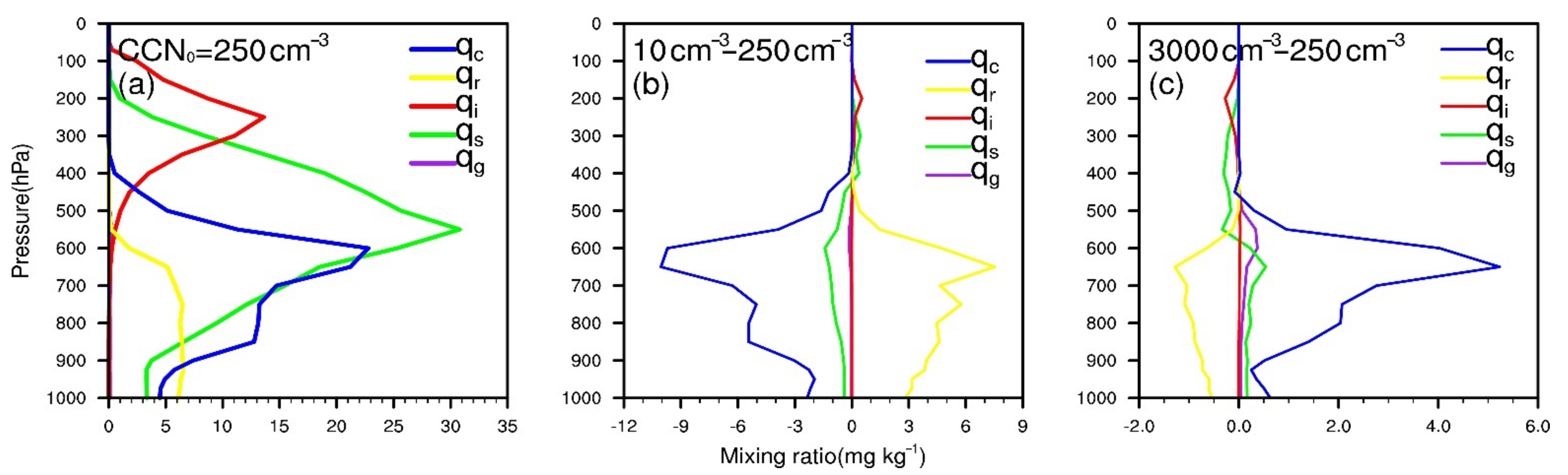
4.1. The CCN Impacts on the Mass Mixing Ratio of Hydrometeors

Firstly, Figure 2 gives the vertical distribution of the average mixing ratio five kinds of hydrometeors, qc, qr, qi, qs, and qg simulated by the Morrison scheme with CCN0 values of 10 cm−3, representing CCN in a clean atmosphere, 250 cm−3 representing typical continent CCN, and 3000 cm−3 representing CCN in the severe polluting atmosphere from 8 to 12 October 2017. The black line is the 0° temperature line at the height of about 600 hPa.
It can be seen from Figure 2 that qc gets to the maximum value from 04:00 UTC to 19:00 UTC on 9 October from the height of 800 hPa to 650 hPa with CCN0 values of 10 cm−3. The qc gets to the maximum value at a height of 600 hPa from 6:00 UTC to 18:00 UTC on 9 October with CCN0 values of 250 cm−3. With values of CCN0 varying to 3000 cm−3, qc increases significantly, and the increase in CCN0 enhances qc by 133%. The qr gets to the maximum value after 11:00 UTC on 9 October at the height of 950 hPa to 750 hPa; qr decreases with values of CCN0 increasing to 250 cm−3, and the ground gets to a maximum value at the height from land layer to 700 hPa during the period of 13:00 UTC on 9 October to 02:00 UTC on 10 October. With the values of CCN0 increasing to 3000 cm−3, qr has a large reduction significantly. After 14:00 UTC on 9 October, qr decreases by 44% compared with 10 cm−3. Figure 3 displays the vertical profiles of the region and period averaged qc, qr, qi, qs, qg with CCN0 of 250 cm−3 (a) and the differences between it and that of CCN0 of 10 cm−3 (b) and 3000 cm−3 (c). It can be seen clearly that comparing Figure 3a–c when CCN0 is set as 10 cm−3, qc decreases and qr increases comparing with those when CCN0 is 250 cm−3; the maximum of the qc differences between the two is up to 10 mg/kg, which is an account for 43% of the maximum value of qc when CCN0 is 250 cm−3. Correspondingly, the maximum of qr decrease is 6, accounting for almost 100% of qr when CCN0 is set as 250 cm−3. Conversely, when CCN0 is set as 3000 cm−3, qc increases and qr decreases comparing with those when CCN0 is 250 cm−3. The maximum of the qc differences between the two is about 5 mg/kg, which means about a 22% increase of the maximum value of qc when CCN0 is 250 cm−3, and the maximum qr decrease is about 20%.
However, comparing with qc and qr, the changes of qi and qs due to the CCN0 changing is small (Figure 2). The sources of cloud ice crystals are mainly from the ice nucleation from freezing of aerosol and the heterogeneous freezing of droplets, among which ice nucleation from the freezing of aerosol is more important [16,22]. When CCN number concentration increases, the impact on the ice nuclei is little, and the largest source of ice crystal is not changed [67]. Moreover, because the cloud system studied here is a stratus cloud with few ascending motions, it is difficult to freeze a large amount of cloud water. Based on these, the number concentration of CCN changes will not change the ice crystals much. Meantime, the source of snow and graupel is ice crystals [68]. Therefore, compared with cloud water and cloud raindrops, the changes of cloud ice, cloud snow, and graupel are not obvious. Although this change is small, the mixing ratio of cloud snow and graupel also changes to a certain extent with the increase of the CCN concentration, which is manifested as a rise near and below the 0 °C isotherm and a drop in the upper air slightly (Figure 3). This result agrees with the studies that the increase of CCN is not conducive to the formation of ice particles in the upper air [16,17,18,19,22,36,37]. The reason may be that the increase of cloud droplets consumes ice crystals and causes them to fall above 0 °C isotherm. In addition, the increase of CCN causes the cloud water to rise significantly near the 0 °C isotherm, which is beneficial to the growth of the snow and graupel. Therefore, the mixing ratio of cloud snow and graupel increase with CCN increasing below 500 hPa.

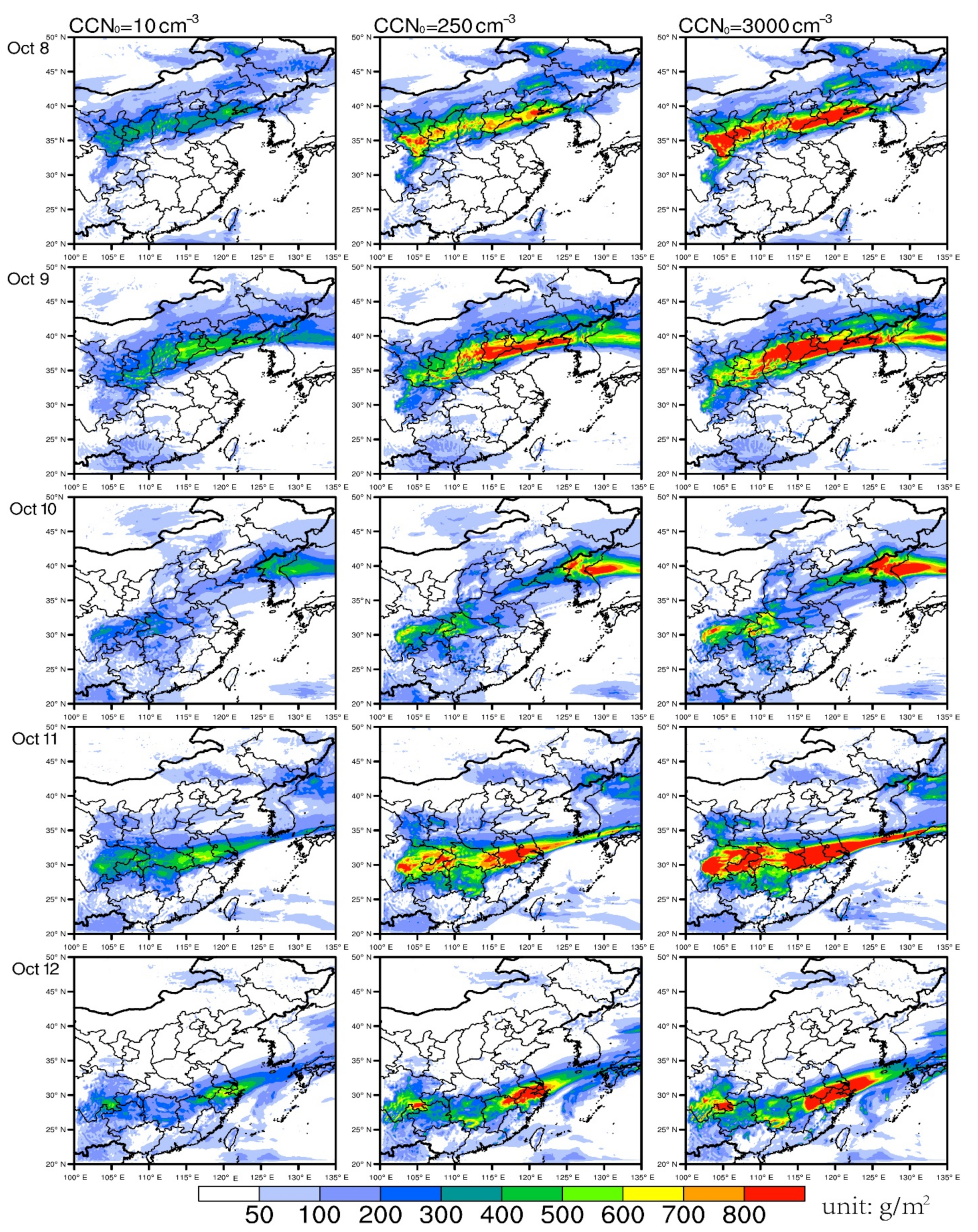
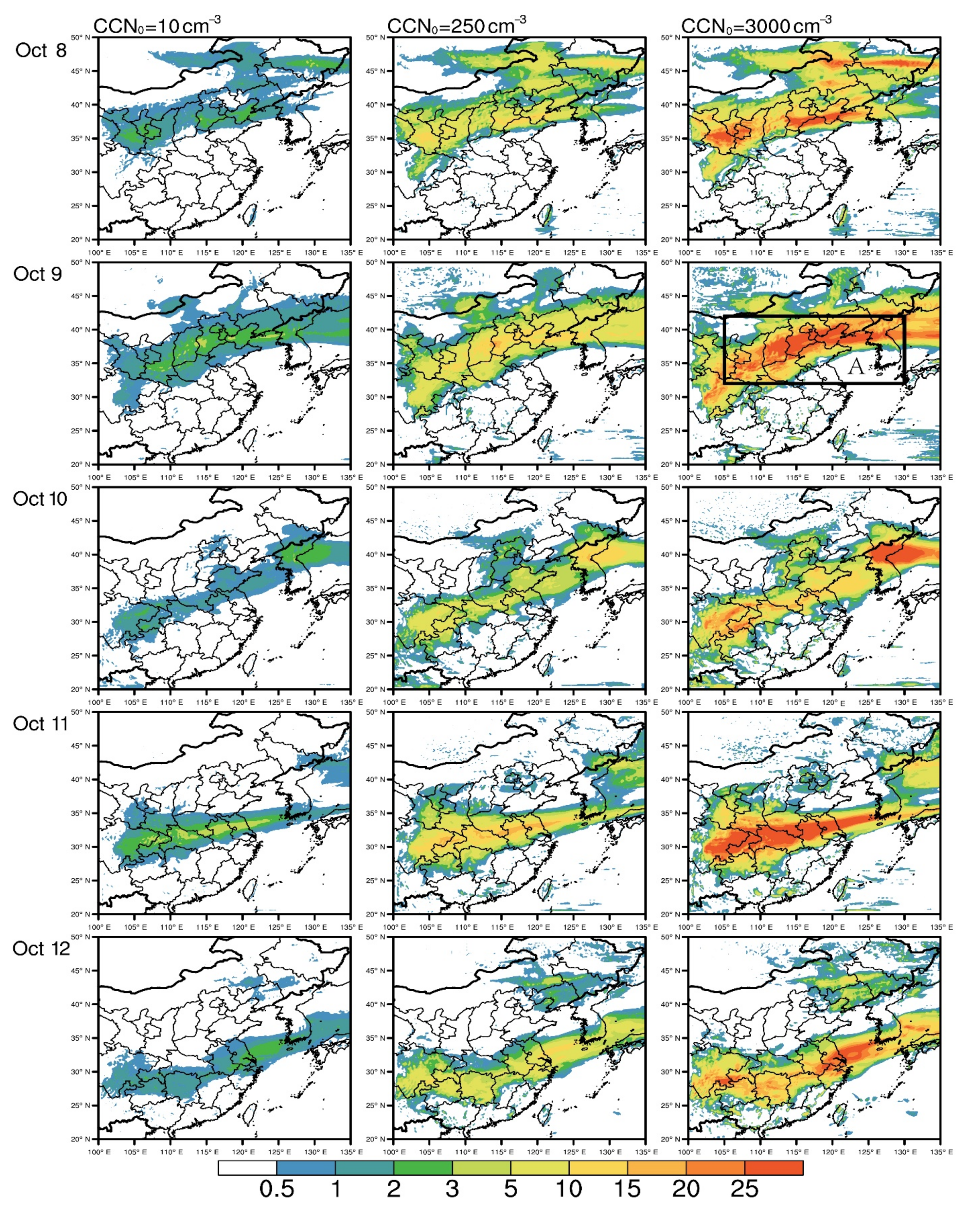
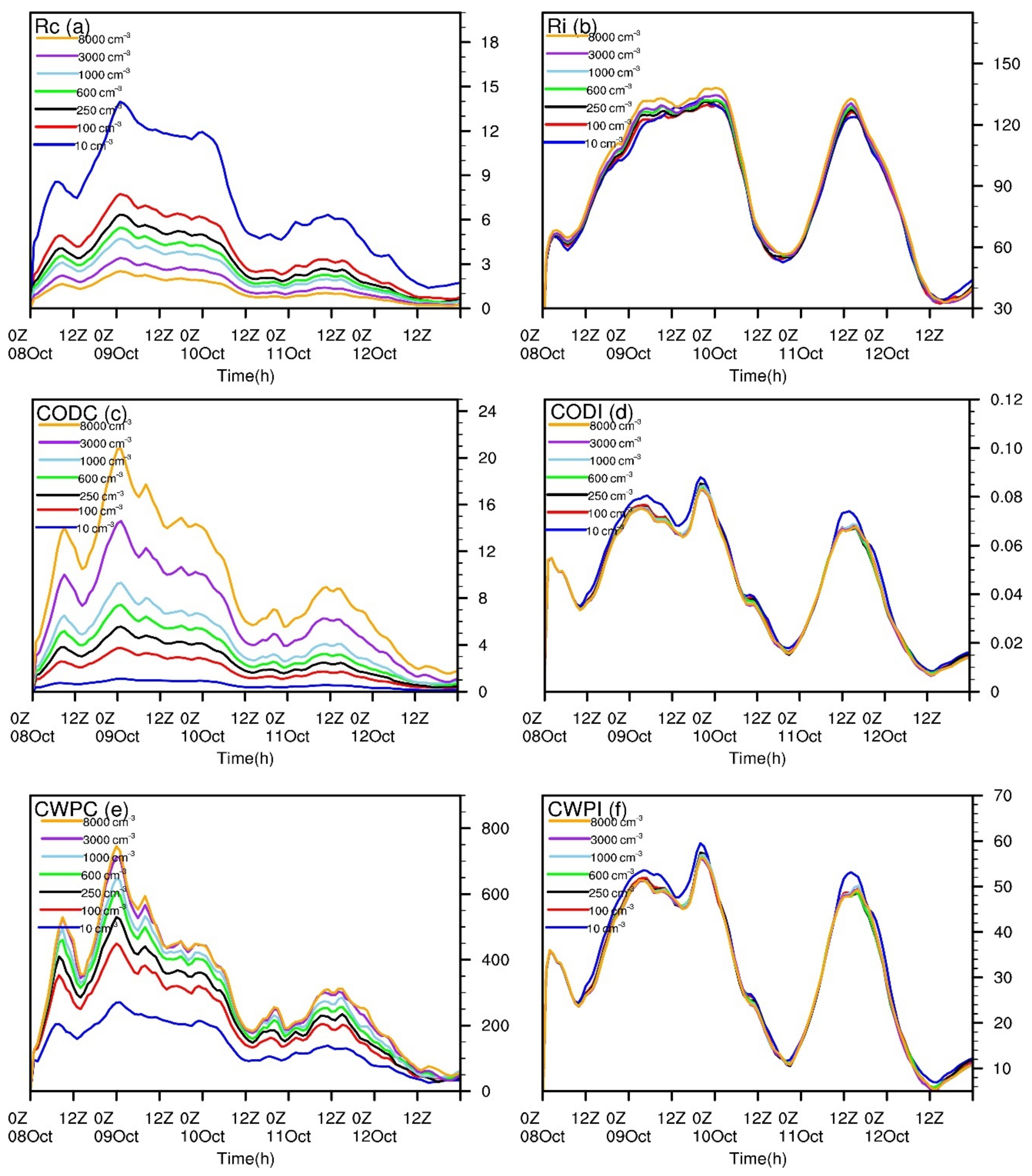
4.2. CCN Impacts on Modeled Rc, CLWP, and COD

CLWP represents the total cloud water atmosphere column loading and has an important influence on the total cloud radiation process. Rc, the cloud particle size, is the very sensitive parameter on the cloud optical features and on the cloud radiation process. COD is the direct input parameter combining the contributions of cloud water loading and optical impacts in the radiative transfer model to calculate the cloud radiation process [64].
Figure 4 shows the simulated daily Rc from 8 October to 12 October when CCN0 is set as 10, 250, and 3000 cm−3 in Morrison scheme. It can be seen from Figure 4 that there are distinguished differences among the simulated Rc of the three CCN0 values. In general, Rc decreases with the CCN0 increasing, and Rc is the biggest when CCN0 is set as 10 cm−3; the second corresponds to CCN0 of 250 cm−3, and the smallest corresponds to CCN0 of 3000 cm−3. Although the Rc’s differences between CCN0 of 10 cm−3 and 250 cm3, representing the possible Rc’s differences between very clean and normal continent CCN0, are much bigger than those between CCN0 of 250 cm−3 and 3000 cm−3, representing the Rc’s differences between normal continent CCN0 and CCN0 of severe pollution atmosphere, the Rc’s differences between CCN0 of 250 cm−3 and 3000 cm−3 are still obvious enough to show the possible reforming on Rc due to the CCN0 changing from normal continent atmosphere to severe pollution atmosphere. The maximum value of daily average Rc decreases by about 63% when CCN0 increases from 10 cm−3 to 3000 cm−3. It is worth noting that for CLWP (Figure 5), the changes in CLWP are consistent with CCN0, but the magnitude of increase in CLWP is much smaller than the increase in CCN0 with getting smaller tendency. In this case, in which the increase in cloud water content is relatively low, too many cloud droplets compete for water and are not prone to growth, which will lead to rapid decrease in Rc and the magnitude of the decrease decreases [69].
Figure 5 displays the daily average CLWP by the model from 8 to12 October when CCN0 is 10, 250, and 3000 cm−3 in Morrison scheme in the model run. It can be seen that CLWP corresponding CCN0 of 10 cm−3 is the smallest, CLWP corresponding CCN0 of 250 cm−3 is the second, and CLWP corresponding CCN0 of 3000 cm−3 is the biggest, illustrating that more CCN0 results in less Rc (Figure 4) and the automatic conversion process from cloud to rain, and more cloud water exits in the atmosphere. The maximum value of daily average CLWP increases by 100% when the values of CCN0 going from 10 cm−3 to 3000 cm−3. Comparing the CLWPs under the three CCN0 values, it can be found that the CLWP differences between CCN0 as 10 and 250 cm−3 are bigger than those between CCN0 as 250 and 3000 cm−3 under the same background of atmospheric circulation and water vapor. Model daily COD (Figure 6) shows a similar change with the CCN0 changing, that is, COD with CCN0 as 10 cm−3 is the smallest, COD with CCN0 as 250 cm−3 is the middle, and COD with CCN0 as 3000 cm−3 is the biggest. The maximum value of daily average COD increases by 150% when the values of CCN0 go from 10 cm−3 to 3000 cm−3. COD has a good positive correlation with CLWP. The bigger the cloud water content is, the greater the cloud optical depth is, which causes the less solar shortwave radiation received by the ground [69]. However, there is still a certain difference between the CLWP and COD changing with the CCN0, that is, COD changes more with CCN0 from 250 to 3000 cm−3 than CLWP did. This suggests that COD increases much more with CCN0 changing from normal continent (250 cm−3) to severe pollution CCN0 (3000 cm−3) than CLWP does. This can be interpreted as that CLWP is only changed by the changes of cloud water mixing by CCN0, but COD may be changed by both the changes of cloud water mixing and optical properties of cloud particles due to the cloud size changing. When CCN0 changes from 10 to 250 cm−3, the cloud particle size is relatively big; the impact of CCN0 on cloud water content is bigger than that on optical features of cloud particles, and thus the CLWP difference is bigger than COD. When CCN0 changes from 250 to 3000 cm−3, the cloud particle size is much smaller; the impact of CCN0 on optical features of cloud particles is much more important than it on cloud water content, and thus, the COD difference is bigger than CLWP. This result suggests the possible COD difference due to normal continent CCN0 and severe pollution CCN0.
The above discussion uses three CCN0 values of 10 (representing very clean atmosphere), 250 (representing continent atmosphere), 3000 cm−3 (representing severe pollution atmosphere) in the Morrison scheme to discuss the CCN impacts on cloud properties. However, in the real atmosphere, CCN varies with meteorological conditions and aerosols types and concentrations. The experiment results when CCN is set as 10, 100, 250, 600, 1000, 3000, or 8000 cm−3 will be used to discuss the different CCN values on cloud properties in detail. Hence, Region A (32°–42° N, 105°–130° E) is chosen to study the effect of different values of CCN on area-averaged cloud microphysical quantities.
Figure 7 displays the temporal changing of region averaged Rc, Ri, CODC, CODI, CLWP of cloud water (CWPC), and CLWP of cloud ice (CWPI) corresponding to the different CCN0 from 8 to 12 October. It can be seen that Rc (Figure 7a) decreases, while CODC (Figure 7c) and CWPC (Figure 7e) increase with the CCN0 increasing from 10, 100, 250, 600, 1000, 3000, to 8000 cm−3. This is mainly because more CCN in the atmosphere leads to a smaller size of cloud particles (smaller Rc), less auto conversion from cloud to rain, more water cloud with smaller particle sizes in the atmosphere, and higher atmospheric column cloud water, which means bigger CODC and CWPC. Among the Rc differences between every two adjacent CCN0 values, the difference between Rc when CCN0 is set as 10 cm−3 and that when CCN0 is 250 cm−3 is the biggest. Though CODC and CWPC show similar changes with the CCN0, there are still some differences: Similar to Rc changes, the difference between CWPC when CCN0 is set as 10 cm−3 and that when CCN0 is 250 cm−3 is the biggest among the CWPC differences between every two adjacent CCN0 values. CWPC changes with CCN0 from 100, 250, 600, 1000, 3000, to 8000 cm−3 is not as large as it is with CCN0 from 10 to 100 cm−3. However, CODC changing with CCN0 shows certain different features to those of Rc and CWPC, that is, the largest differences in CODC between per two adjacent CCN0 occur in CCN0 changing from 1000 to 3000 cm−3 or 3000 to 8000 cm−3, instead of CCN0 changing from 10 to 100 cm−3 as Rc and CWPC do. In other words, when atmosphere CCN changes from a very clean atmosphere (10 cm−3) to continent atmosphere (100 or 250 cm−3), Rc and CWPC change the most, and COD changes most with CCN continued increases based on pollution atmosphere (from 1000 to 3000, or 8000 cm−3). Furthermore, COD changes uniformly with CCN0 changing from 10, 100, 250, 600, 1000, 3000 to 8000 cm−3 while CLWP and Rc change most with CCN0 changing from 10 to 100 cm−3. This is because that CWPC is only affected by atmosphere column cloud water, but COD is affected by both atmosphere column cloud water and optical features of cloud particle sizes. Comparing with water cloud, ice cloud parameters including Ri (Figure 7b), CODI (Figure 7e), and CWPI (Figure 7f) change slightly with CCN0.

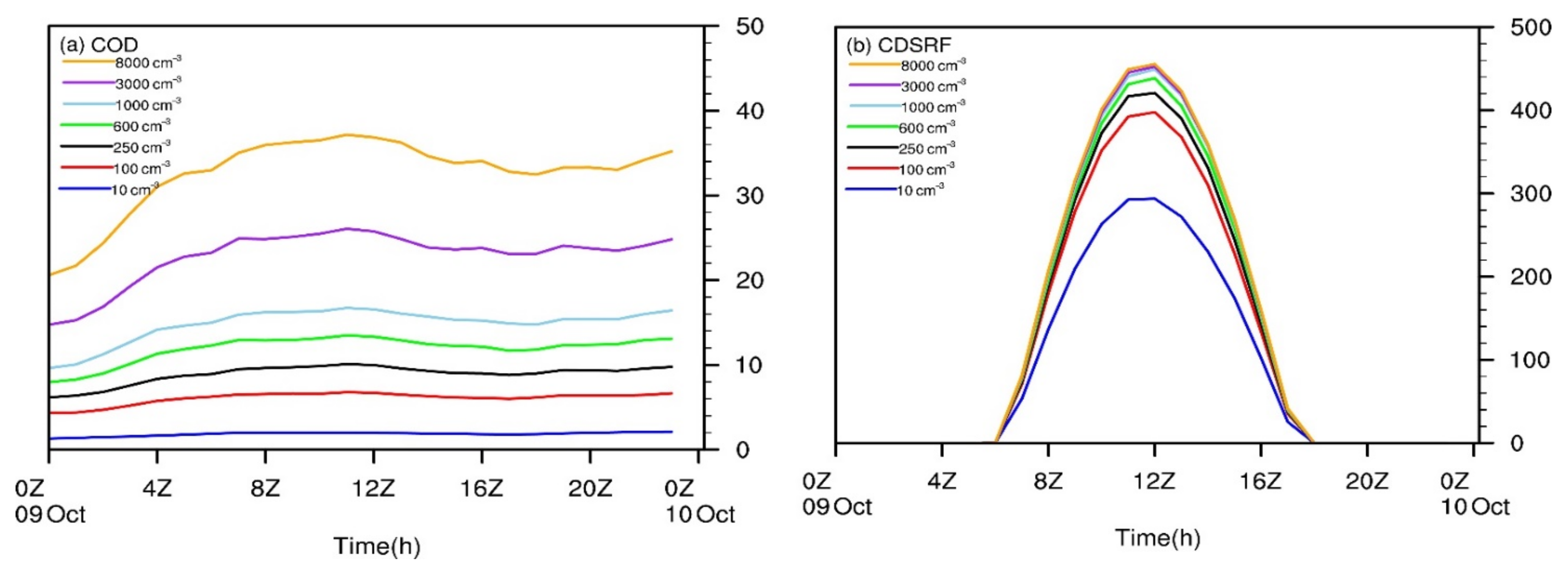
4.3. CCN Impacts on Cloud Radiation Forcing

The discussion in the above section illustrates the important impacts of CCN changing on cloud features, especially on water cloud features, which is sure to lead the changes in the cloud radiation process. The increase in number concentration and the decrease in size of cloud droplets will lead to increase of cloud albedo (Twomey effect). In addition, the decrease in particle size will reduce the precipitation rate and increase the liquid water content in the cloud, the thickness of the cloud, and the life of the cloud (Albrecht effect). These processes will change cloud albedo, resulting in the decrease of solar shortwave radiation received by the ground [3,70]. The cloud downward shortwave radiative forcing (CDSRF) provides a means to quantify the effect of cloud on radiation. The CDSRF is calculated by the Equation (3):
C D S R F = F c l e a r s w F c l o u d y s w
where F s w is the simulated downward shortwave radiation received by the surface. The subscripts “clear” and “cloudy” refer to clear-sky and cloudy (all-sky) conditions.
Figure 8 shows CDSRF at 12:00 UTC from 8 to 12 October 2017 when CCN0 is 250 cm−3 and the difference between it and that when CCN0 is 10 cm−3 or 3000 cm−3. It can be seen that there are distinguished differences among the simulated CDSRF of the three CCN0 values. In general, CDSRF with CCN0 as 10 cm−3 is the smallest, CDSRF with CCN0 as 250 cm−3 is the middle, and CDSRF with CCN0 as 3000 cm−3 is the biggest. When CCN0 is set as 10 cm−3, CDSRF increases comparing with that when CCN0 is 250 cm−3; the maximum of the CDSRF differences between the two is up to −220 W/m2, which decrease by about 37% compared with the maximum value of CDSRF when CCN0 is 250 cm−3. Conversely, when CCN0 is set as 3000 cm−3, the maximum of the CDSRF differences between the two is about 60 W/m2, which means about 10% increasing of the maximum value of CDSRF when CCN0 is 250 cm−3. Comparing the CDSRFs under the three CCN0 values, it can be found that the possible CDSRF differences between very clean and normal continent CCN0 are much bigger than CDSRF differences between normal continent CCN0 and CCN0 of severe pollution atmosphere. The maximum value of daily average CDSRF differences between CCN0 of 10 cm−3 and 3000 cm−3 is up to 260 W/m2, which means about a 65% increasing of the maximum value of daily average CDSRF when CCN0 is 10 cm−3.
Figure 9 displays hourly area-averaged COD (Figure 9a) and CDSRF (Figure 9b) of Region A at 12:00 UTC corresponding to the different CCN0 on 9 October 2017. It can be seen that COD and CDSRF increases with the CCN0 increasing from 10, 100, 250, 600, 1000, 3000, to 8000 cm−3. The area-averaged COD and CDSRF get to the maximum value at 12:00 UTC on 9 October; this is mainly because higher COD leads to higher CDSRF. Among the CDSRF differences between every two adjacent CCN0 values, the differences between CDSRF when CCN0 is set as 10 cm−3 and that when CCN0 is 100 cm−3 is the biggest. However, COD changing with CCN0 shows a certain different feature with those of CDSRF, that is, the largest differences in COD between per two adjacent CCN0 occur when CCN0 changes from 3000 to 8000 cm−3, instead of those in CDSRF when CCN0 changes from 10 to 100 cm−3. In other words, when atmosphere CCN changes from 10 to 100 or 250 cm−3, CDSRF changes the most, while COD changes most when CCN continues to increase from 1000 to 3000 or 8000 cm−3.
Table 4 displays area-averaged CDSRF of Region A with CCN changing and their percentage changes compared with CCN0 (250 cm−3) at 12:00 UTC from 8 to 12 October. CDSRF changes the most with CCN0 changing from 10 to 250 cm−3 on 9 October, and the maximum of the area-averaged CDSRF differences between the two is up to −80.8W/m2, which decrease by 28.9% compared with the maximum value of CDSRF when CCN0 is 250 cm−3. The maximum percentage change is up to 40.6% between 10 cm−3 and 250 cm−3 on 8 October, while the minimum of that is 3% between 250 cm−3 and 600 cm−3 on the same day. When atmosphere CCN changes from very clean atmosphere (10 cm−3) to continent atmosphere (250 cm−3), the percentage change compared to CDSRF with CCN0 set as 250 cm−3 is between 23.0% and 40.6%; when the CCN0 changing from normal continent atmosphere (250 cm−3) to severe pollution atmosphere (3000 cm−3), the percentage change is between 6.5% and 11.6%. Particularly, the values of area-averaged CDSRF of Region A in Table 1 are smaller than those in Figure 8, this is because the distribution of daily average CDSRF is uneven in Region A.

5. Summary and Conclusions

The Morrison double-moment cloud microphysical scheme including mass and droplets number concentration of water and ice cloud is integrated into the GRAPES_Meso model and a large-area stratus cloud process from 00:00 UTC 8 October to 00:00 UTC 13 October 2017 is simulated by it. The MODIS Rc, COD, and NCEP reanalysis CLWP are used for model evaluation. Sensitivity experiments are performed with different values of CCN number concentration varying from 10, 100, 250, 600, 1000, 3000, to 8000 cm−3, respectively, to study the effects of CCN on microphysics processes and cloud radiation effect in East China. The specific conclusions of the paper are summarized as follows.
Compared with WDM6 scheme in GRAPES_Meso, Morrison scheme has better performance in simulating the cloud microphysical characteristics in this study. The simulated CLWP shows a great agreement with that of NCEP reanalysis. Both the regional distribution and magnitude of simulated Rc and COD are consistent with those retrieved by MODIS satellite, indicating that the reasonability and availability of the Morrison scheme in the cloud description of cloud optical properties and radiation in GRAPES_Meso in East Asia.
With the values of CCN0 increasing from 10 cm−3 (representing a very clean atmosphere) to 3000 cm−3 (representing severe pollution atmosphere), the maximum value of daily average Rc decreases by 63%, while the impact of CCN has a little effect on Ri. Besides, the maximum value of the simulated daily average qc increases by about 133%, the maximum value of daily average qr decreases by 44%, the maximum value of daily average CLWP increases by 100%, and the maximum average COD increases by 150% while the CWPI and CODI decrease slightly. Because ice nuclei (the largest source of ice crystal) have not been changed, and the cloud system studied here is a stratus cloud with few ascending motions, it is difficult to freeze a large amount of cloud water. Based on these, the number concentration of CCN changes will not change the ice crystals much. Meanwhile, the source of snow and graupel are ice crystals. Therefore, compared with cloud water and cloud raindrops, the changes of cloud ice, cloud snow, and graupel are not obvious. When the number concentration of CCN0 exceeds 3000 cm−3, its impact on CLWP is small, but the impact on COD is big due to the combined impacts of CCN on cloud water and cloud optical features related to particle size. These processes will change cloud albedo when CCN0 increases, resulting in the decrease of solar shortwave radiation received by the ground. The maximum value of daily average CDSRF increases by 65% on 9 October. CDSRF changes the most when atmosphere CCN changes from 10 cm−3 to 100 or 250 cm−3. For the uneven distribution of daily average CDSRF in Region A, the values of area-averaged CDSRF of Region A are smaller than the values of daily averaged CDSRF. These study results show CCN’s important impacts on cloud properties and radiative forcing. Because of the complexity of the effect of CCN on clouds, further studies will focus on more cloud processes and types, more microphysical schemes, and CCN or ice cloud nucleation (IN) activation.

Supplementary Materials

The following are available online at https://www.mdpi.com/article/10.3390/atmos12040489/s1, Figure S1: Comparation between MODIS and CCN = 250 cm−3 Rc from 23 to 28 October 2017, Figure S2: Comparation between MODIS and CCN = 250 cm−3 COD from 23 to 28 October 2017, Figure S3: Comparation between NCEP and CCN = 250 cm−3 CLWP from 23 to 28 October 2017, Figure S4: Averaged Rc (μm) from 5 to 7 January 2017 (Left: MODIS data; Mid: WDM6 Scheme; Right: Morrison Scheme), Figure S5: Averaged COD from 5 to 7 January 2017 (Left: MODIS data; Mid: WDM6 Scheme; Right: Morrison Scheme), Figure S6: Averaged CLWP (g m−2) from 5 to 7 January 2017 (Left: NCEP data; Mid: WDM6 Scheme; Right: Morrison Scheme), Table S1: Comparison of observed and average Rc, COD and CLWP with CCN values of 250 cm−3 simulated by Morrison and WDM6 scheme from 5 to 7 January 2017.

Author Contributions

Conceptualization, H.W.; methodology, H.W. and M.Z.; data curation, X.Z.; writing—original-draft preparation, Y.S.; writing—review and editing, H.W. and W.Z.; visualization, Y.P. and Z.L.; project administration, H.W.; funding acquisition, H.W., X.S. and J.H. All authors have read and agreed to the published version of the manuscript.

Funding

This research was fundedby the National Key Research and Development Project (2019YFC0214601) and the National Natural Science Foundation of China (41590874, 41975054, 41930967).

Institutional Review Board Statement

Not applicable.

Informed Consent Statement

Not applicable.

Data Availability Statement

Not applicable.

Acknowledgments

We appreciate the provision of the NCEP/NCAR reanalysis data from the National Center for Meteorological and Environmental Forecast (NCEP) and National Center for Atmospheric Research (NCAR) (https://rda.ucar.edu/datasets/ (accessed on 20 July 2019)), and MODIS data from The Land Processes Distributed Active Archive Center (https://ladsweb.modaps.eosdis.nasa.gov/ (accessed on 20 July 2019)).

Conflicts of Interest

The authors declare no conflict of interest.

References

  1. Stephens, G.L. Cloud feedbacks in the climate system: A critical review. J. Clim. 2005, 18, 237–273. [Google Scholar] [CrossRef] [Green Version]
  2. Duan, J.; Liu, Y. Trends of cloud optical depth and cloud effective radius variation in China. J. Meteorol. Sci. Technol. 2011, 39, 408–416. (In Chinese) [Google Scholar]
  3. Ackerman, A.S.; Toon, O.B.; Taylor, J.P.; Johnson, D.W.; Hobbs, P.V.; Ferek, R.J. Effects of aerosols on cloud albedo: Evaluation of Twomey’s parameterization of cloud susceptibility using measurements of ship tracks. J. Atmos. Sci. 2000, 57, 2684–2695. [Google Scholar] [CrossRef] [Green Version]
  4. Yin, J.; Wang, D.; Zhai, G. Long-term in situ measurements of the cloud-precipitation microphysical properties over East Asia. J. Atmos. Res. 2011, 102, 206–217. [Google Scholar] [CrossRef]
  5. Clark, T.L. Numerical modeling of the dynamics and microphysics of warm cumulus convection. J. Atmos. Sci. 1973, 30, 857–878. [Google Scholar] [CrossRef]
  6. Takahashi, T. Tropical showers in an axisymmetric cloud model. J. Atmos. Sci. 1975, 32, 1318–1330. [Google Scholar] [CrossRef] [Green Version]
  7. Garvert, M.F.; Woods, C.P.; Colle, B.A.; Mass, C.F.; Hobbs, P.V.; Stoelinga, M.T.; Wolfe, J.B. The 13-14 December 2001 IMPROVE-2 Event. Part II: Comparisons of MM5 model simulations of clouds and precipitation with observations. J. Atmos. Sci. 2005, 62, 3520–3534. [Google Scholar] [CrossRef]
  8. Sarkadi, N.; Geresdi, I.; Thompson, G. Numerical simulation of precipitation formation in the case orographically induced convective cloud: Comparison of the results of bin and bulk microphysical schemes. J. Atmos. Res. 2016, 180, 241–261. [Google Scholar] [CrossRef]
  9. Hall, W.D. A detailed microphysical model within a two-dimensional dynamic framework: Model description and preliminary results. J. Atmos. Sci. 1980, 37, 2486–2507. [Google Scholar] [CrossRef]
  10. Khain, A.P.; Sednev, I. Simulation of precipitation formation in the eastern Mediterranean coastal zone using a spectral microphysics cloud ensemble model. Atmos. Res. 1996, 43, 77–110. [Google Scholar] [CrossRef]
  11. Lin, Y.L.; Farley, R.D.; Orville, H.D. Bulk parameterization of the snow field in a cloud model. J. Appl. Meteorol. Sci. 1983, 22, 1065–1092. (In Chinese) [Google Scholar] [CrossRef] [Green Version]
  12. Mitchell, D.L. A model predicting the evolution of ice particle size spectra and radiative properties of cirrus clouds. Part I: Microphysics. J. Atmos. Sci. 1994, 51, 797–816. [Google Scholar] [CrossRef] [Green Version]
  13. Frick, C.; Seifert, A.; Wernli, H. A bulk parameterization of melting snowflakes with explicit liquid water fraction for the COSMO model. Geosci. Model Dev. 2013, 6, 1925–1939. [Google Scholar] [CrossRef] [Green Version]
  14. Cotton, W.R.; Tripoli, G.J.; Rauber, R.M.; Mulvihill, E.A. Numerical simulation of the effects of varying ice crystal nucleation rates and aggregation processes on orographic snowfall. J. Climate Appl. Meteorol. 1986, 25, 1658–1680. [Google Scholar] [CrossRef] [Green Version]
  15. Reisin, T.; Levin, Z.; Tzivion, S. Rain production in convective clouds as simulated in an axisymmetric model with detailed microphysics. Part, I. Description of the model. J. Atmos. Sci. 1996, 53, 497–519. [Google Scholar] [CrossRef] [Green Version]
  16. Milbrandt, J.A.; Yau, M.K.; Mailhot, J.; Bélair, S. Simulation of an Orographic Precipitation Event during IMPROVE-2. Part I: Evaluation of the Control Run Using a Triple-Moment Bulk Microphysics Scheme. Mon. Weather Rev. 2008, 136, 3873–3893. [Google Scholar] [CrossRef]
  17. Ferrier, B.S. A double-moment multiple-phase four-class bulk ice scheme, Part 1: Description. J. Atmos. Sci. 1994, 51, 249–280. [Google Scholar] [CrossRef] [Green Version]
  18. Gao, W.; Zhao, F.; Hu, Z.; Feng, X. A two-moment bulk microphysics coupled with a mesoscale model WRF: Model description and first results. J. Adv. Atmos. Sci. 2011, 28, 1184–1200. [Google Scholar] [CrossRef]
  19. Zheng, X.; Albrecht, B.; Minnis, P.; Ayers, K.; Jonson, H.H. Observed aerosol and liquid water path relationships in marine stratocumulus. Geophys. Res. Lett. 2010, 37. [Google Scholar] [CrossRef] [Green Version]
  20. Zhou, C.H.; Gong, S.; Zhang, X.Y.; Liu, H.L.; Xue, M.; Cao, G.L.; An, X.Q.; Che, H.Z.; Zhang, Y.M.; Niu, T. Towards the improvements of simulating the chemical and optical properties of Chinese aerosols using an online coupled model-CUACE/Aero. Tellus B 2012, 64, 18965. [Google Scholar] [CrossRef] [Green Version]
  21. Wang, Z.L.; Zhang, H.; Lu, P. Improvement of cloud microphysics in the aerosol-climate model BCC_AGCM2.0.1_CUACE/Aero, evaluation against observations, and updated aerosol indirect effect. J. Geophys. Res. Atmos. 2014, 119, 8400–8417. [Google Scholar] [CrossRef]
  22. Morrison, H.; Curry, J.A.; Khvorostyanov, V.I. A new double-moment microphysics parameterization for application in cloud and climate models, Part I: Description. J. Atmos. Sci. 2005, 62, 1665–1677. [Google Scholar] [CrossRef]
  23. He, T.; Zhao, F.S. An improved retrieval algorithm of aerosol optical depth. J. Appl. Meteorol. Sci. 2011, 22, 663–672. (In Chinese) [Google Scholar]
  24. Dong, H.; Xu, H.M.; Luo, Y.L. Effects of cloud condensation nuclei concentration on precipitation in convection permitting simulations of a squall line using WRF model: Sensitivity to cloud microphysical schemes. Chin. J. Atmos. Sci. 2012, 36, 145–169. (In Chinese) [Google Scholar]
  25. Shen, X.Y.; Mei, H.X.; Wang, W.G.; Huang, W.Y. Numerical simulation of ice-phase processes using a double-moment microphysical scheme and a sensitivity test of ice nuclei concentration. Chin. J. Atmos. Sci. 2015, 39, 83–99. (In Chinese) [Google Scholar]
  26. Baró, R.; Jiménez-Guerrero, P.; Balzarini, A.; Curci, G.; Forkel, R.; Grell, G.; Hirtl, M.; Honzak, L.; Langer, M.; Pérez, J.L.; et al. 2015: Sensitivity analysis of the microphysics scheme in WRF-Chem contributions to AQMEII phase 2. J. Atmos. Environ. 2015, 115, 620–629. [Google Scholar] [CrossRef]
  27. Li, G.; Wang, Y.; Zhang, R. Implementation of a two-moment bulk microphysics scheme to the WRF model to investigate aerosol-cloud interaction. J. Geophys. Res. 2008, 113, 1139. [Google Scholar] [CrossRef]
  28. Morrison, H.; Milbrandt, J.A. Parameterization of cloud microphysics based on the prediction of bulk ice particle properties. Part I: Scheme description and idealized tests. J. Atmos. Sci. 2015, 72, 287–311. [Google Scholar] [CrossRef]
  29. Thompson, G.; Field, P.R.; Rasmussen, R.M.; Hall, W.D. Explicit forecasts of winter precipitation using an improved bulk microphysics scheme. Part II: Implementation of a new snow parameterization. Mon. Weather Rev. 2008, 136, 5095–5115. [Google Scholar] [CrossRef]
  30. Thompson, G.; Rasmussen, R.M.; Manning, K. Explicit forecasts of winter precipitation using an improved bulk microphysics scheme. Part I: Description and sensitivity analysis. Mon. Weather Rev. 2004, 132, 519–542. [Google Scholar] [CrossRef] [Green Version]
  31. Thompson, G.; Eidhammer, T. A study of aerosol impacts on clouds and precipitation development in a large winter cyclone. J. Atmos. Sci. 2014, 71, 3636–3658. [Google Scholar] [CrossRef]
  32. Heinzeller, D.; Junkermann, W.; Kunstmann, H. Anthropogenic aerosol emissions and rainfall decline in southwestern Australia: Coincidence or causality? J. Clim. 2016, 29, 8471–8493. [Google Scholar] [CrossRef] [Green Version]
  33. Reshmi Mohan, P.; Srinivas, C.V.; Yesubabu, V.; Baskaran, R.; Venkatraman, B. Simulation of a heavy rainfall event over Chennai in Southeast India using WRF: Sensitivity to microphysics parameterization. Atmos. Res. 2018, 210, 83–99. [Google Scholar] [CrossRef]
  34. Jiang, H.; Feingold, G. Effect of aerosol on warm convective clouds: Aerosol-cloud-surface flux feedbacks in a new coupled large eddy model. J. Geophys. Res. 2006, 111. [Google Scholar] [CrossRef]
  35. Ochs, H.T.; Yao, C.S. Moment-conserving techniques for warm cloud microphysical computations. Part I: Numerical techniques. J. Atmos. Sci. 2010, 35, 1947–1958. [Google Scholar] [CrossRef] [Green Version]
  36. Li, Y.W.; Quan, X.; Zhang, Z.F. Numerical research of CCN concentration and its paramreterization scheme’s influence on a stratiform precipitation process. Trans. Atmos. Sci. 2018, 184, 119–130. (In Chinese) [Google Scholar]
  37. O’Sullivan, P.B.; Phyty, G.D.; Twomey, L.T. Evaluation of specific stabilizing exercise in the treatment of chronic low back pain with radiologic diagnosis of spondylolysis or spondylolisthesis. Spine 1997, 22, 2959–2967. [Google Scholar] [CrossRef]
  38. Klaus, W. The Effective Radius in Ice Clouds. J. Clim. 1997, 11, 1793–1802. [Google Scholar]
  39. Yang, B.Y.; Zhang, H.; Peng, J.; Wang, Z.L.; Jing, X.W. Analysis on Global Distribution Characteristics of Cloud Microphysical and Optical Properties Based on the CloudSat Data. Plateau Weather 2014, 33, 1105–1118. [Google Scholar]
  40. Chen, D.H.; Shen, X.S. Recent progress on GRAPES research and application. J. Appl. Meteorol. Sci. 2006, 17, 773–777. (In Chinese) [Google Scholar]
  41. Wu, X.J.; Jin, Z.Y.; Huang, L.P.; Chen, D.H. The software framework and application of GRAPES model. J. Appl. Meteorol. Sci. 2005, 16, 539–546. (In Chinese) [Google Scholar]
  42. Chen, D.H.; Xue, J.S.; Yang, X.S.; Zhang, H.L.; Shen, X.S.; Hu, J.L.; Wang, Y.; Ji, L.R.; Chen, J.B. New generation of multi-scale NWP system (GRAPES): General scientific design. Chin. Sci. Bull. 2008, 53, 3433–3445. (In Chinese) [Google Scholar] [CrossRef] [Green Version]
  43. Xu, G.Q.; Chen, D.H.; Xue, J.S.; Sun, J.; Shen, X.S.; Shen, Y.F.; Hung, L.P.; Wu, X.J.; Zhang, H.L.; Wang, S.Y. The program structure designing and optimizing tests of GRAPES physics. Chin. Sci. Bull. 2008, 53, 3470–3476. [Google Scholar] [CrossRef] [Green Version]
  44. Zhang, R.H.; Shen, X.S. On the development of the GRAPES—A new generation of the national operational NWP system in China. Chin. Sci. Bull. 2008, 53, 3429–3432. [Google Scholar] [CrossRef] [Green Version]
  45. Zheng, Z.Z.; Zhang, W.C.; Xu, J.W.; Zhao, L.N.; Chen, J.; Yan, Z.W. Numerical simulation and evaluation of a new hydrological model coupled with GRAPES. J. Meteorol. Res. 2012, 26, 653–663. [Google Scholar] [CrossRef]
  46. Zhou, C.H.; Shen, X.J.; Liu, Z.R.; Zhang, Y.M.; Xin, J.Y. Simulating aerosol size distribution and mass concentration with simultaneous nucleation, condensation/coagulation, and deposition with the GRAPES–CUACE. J. Meteorol. Res. 2018, 32, 265–278. [Google Scholar] [CrossRef]
  47. Wang, H.; Xue, M.; Zhang, X.Y.; Liu, H.L.; Zhou, C.H.; Tan, S.C.; Che, H.Z.; Chen, B.; Li, T. Mesoscale modeling study of the interactions between aerosols and PBL meteorology during a haze episode in Jing–Jin–Ji (China) and its nearby surrounding region—Part 1: Aerosol distributions and meteorological features. Atmos. Chem. Phys. 2015, 15, 3257–3275. [Google Scholar] [CrossRef] [Green Version]
  48. Nie, H.H.; Liu, Q.J.; Ma, Z.S. Simulation and analysis of heavy precipitation using cloud microphysical scheme coupled with high-resolution GRAPES model. Meteorol. Mon. 2016, 42, 1431–1444. (In Chinese) [Google Scholar]
  49. Yang, X.; Hu, J.; Chen, D.; Zhang, H.; Shen, X.; Chen, J.; Ji, L. Verification of GRAPES unified global and regional numerical weather prediction model dynamic core. Chin. Sci. Bull. 2008, 53, 3458–3464. [Google Scholar] [CrossRef] [Green Version]
  50. Rosenkranz, P.W. Rapid radiative transfer model for AMSU/HSB channels. IEEE Trans. Geosci. Remote Sens. 2003, 41, 362–368. [Google Scholar] [CrossRef]
  51. Mielikainen, J.; Huang, B.; Huang, H.L.A.; Goldberg, M.D. GPU acceleration of the updated Goddard shortwave radiation scheme in the weather research and forecasting (WRF) Model. IEEE J. Sel. Top. Appl. Earth Obs. Remote Sens. 2012, 5, 555–562. [Google Scholar] [CrossRef]
  52. Johansson, C.; Smedman, A.S.; Högström, U.; Brasseur, J.G.; Khanna, S. Critical test of the validity of Monin-Obukhov similarity during convective conditions. J. Atmos. Sci. 2011, 58, 1549–1566. [Google Scholar] [CrossRef]
  53. Ek, M.B. Implementation of Noah land surface model advances in the national centers for environmental prediction operational mesoscale Eta model. J. Geophys. Res. Atmos. 2003, 108, 8851. [Google Scholar] [CrossRef]
  54. Janjić, Z.I. Comments on “Development and evaluation of a convection scheme for use in climate models”. J. Atmos. Sci. 2000, 57, 3686. [Google Scholar] [CrossRef]
  55. Hong, S.Y.; Pan, H.L. Nonlocal boundary layer vertical diffusion in a medium-range forecast Model. J. Mon. Weather Rev. 1996, 124, 2322. [Google Scholar] [CrossRef] [Green Version]
  56. Morrison, H.; Thompson, G.; Tatarskii, V. Impact of cloud microphysics on the development of trailing stratiform precipitation in a simulated squall line: Comparison of one- and two-moment schemes. Mon. Weather Rev. 2009, 137, 991–1007. [Google Scholar] [CrossRef] [Green Version]
  57. Morrison, H. Modeling clouds observed at SHEBA using a bulk microphysics parameterization implemented into a single-column model. J. Geophys. Res. 2003, 108, 4255. [Google Scholar] [CrossRef]
  58. Morrison, H.; Pinto, J.O. Mesoscale Modeling of Springtime Arctic Mixed-Phase Stratiform Clouds Using a New Two-Moment Bulk Microphysics Scheme. J. Atmos. Sci. 2005, 62, 3683–3704. [Google Scholar] [CrossRef]
  59. Zhang, M.; Wang, H.; Zhang, X.; Peng, Y.; Che, H.Z. 2018: Applying the WRF Double-Moment Six-Class microphysics scheme in the GRAPES_Meso model: A case study. J. Meteorol. Res. 2018, 32, 246–264. [Google Scholar] [CrossRef]
  60. Lu, G.X.; Guo, X.L. Distribution and origin of aerosol and its transform relationship with CCN derived from the spring multi-aircraft measurements of Beijing cloud experiment (BCE). Chin. Sci. Bull. 2012, 57, 2460–2469. [Google Scholar] [CrossRef] [Green Version]
  61. Li, J.X.; Yin, Y.; Ren, G.; Yuan, L.; Li, P.R.; Shen, D.D. Observational study of the spatial-temporal distribution of cloud condensation nuclei in Shanxi Province, China. China Environ. Sci. 2015, 8, 23–33. (In Chinese) [Google Scholar]
  62. Shi, L.X.; Duan, Y. Observations of cloud condensation nuclei in North China. Acta Meteorol. Sin. 2007, 65, 644–652. (In Chinese) [Google Scholar]
  63. Feng, Q.J.; Li, P.R.; Fan, M.Y.; Hou, T.J. Observational analysis of cloud condensation nuclei in some regions of North China. Trans. Atmos. Sci. 2012, 35, 533–540. (In Chinese) [Google Scholar]
  64. Lee, S.S.; Donner, L.J.; Phillips, V.T.J. Cloud and aerosol effects on radiation in deep convective clouds: Comparison with warm stratiform clouds. Atmos. Chem. Phys. 2008, 8, 15291–15341. [Google Scholar]
  65. Ji, Q.; Shaw, G. On supersaturation spectrum and size distributions of cloud condensation nuclei. Geophys. Res. Lett. 1998, 25, 1903–1906. [Google Scholar] [CrossRef]
  66. Fitzgerald, J.W. Dependence of the supersaturation spectrum of ccn on aerosol size distribution and composition. J. Atmos. Sci. 2010, 30, 628–634. [Google Scholar] [CrossRef] [Green Version]
  67. Spice, A.; Johnson, D.W.; Brown, P.R.A.; Darlison, A.G.; Saunders, C.P.R. Primary ice nucleation in orographic cirrus clouds: A numerical simulation of the microphysics. Q. J. R. Meteorol. Soc. 1999, 125, 1637–1667. [Google Scholar] [CrossRef]
  68. Wang, J.; Lee, Y.N.; Daum, P.H.; Jayne, J.; Alexander, M.L. Effects of aerosol organics on cloud condensation nucleus (CCN) concentration and first indirect aerosol effect. Atmos. Chem. Phys. 2008, 8, 6325–6339. [Google Scholar] [CrossRef] [Green Version]
  69. Deng, Z.Z.; Zhao, C.S.; Zhang, Q.; Huang, M.Y.; Ma, X.C. Statistical analysis of microphysical properties and the parameterization of effective radius of warm clouds in Beijing area. Atmos. Res. 2009, 93, 888–896. [Google Scholar] [CrossRef]
  70. Painemal, D.; Zuidema, P. Microphysical variability in southeast Pacific Stratocumulus clouds: Synoptic conditions and radiative response. Atmos. Chem. Phys. 2010, 10, 6255–6269. [Google Scholar] [CrossRef] [Green Version]
Figure 1. Averaged effective radius of cloud water (Rc) (a) (μm), cloud optical depth (COD) (b), and simulated cloud liquid water path (CLWP) (c) (g m−2) (initial CCN number concentration (CCN0) was set as 100, 250, and 300 cm−3 in Morrison scheme) by model and Moderate Resolution Imaging Spectroradiometer (MODIS) Rc, COD, and National Center for Meteorological and Environmental Forecast (NCEP) analysis CLWP from 8 to 12 October 2017.
Atmosphere 12 00489 g001
Figure 2. Temporal changing of vertical profiles of area-averaged qc (ac), qr (df), qi (gi), qs (jl), qg (mo) (mg/kg) from 8 to 12 October (left: CCN0 = 10 cm−3, mid: CCN0 = 250 cm−3, right: CCN0 = 3000 cm−3). The solid black line represents the 0 °C isotherm.
Atmosphere 12 00489 g002
Figure 3. Vertical profiles of area-averaged qc, qr, qi, qs and qg (mg/kg) of A region from 8 to 12 October (a) CCN0 = 250 cm−3, (b) the difference between CCN0 = 10 cm−3 and CCN0 = 250 cm−3, (c) the difference between CCN0 = 3000cm−3 and CCN0 = 250 cm−3).
Atmosphere 12 00489 g003
Figure 4. Daily averaged Rc (μm) by model from 8 to 12 October (left: CCN0 = 10 cm−3, mid: CCN0 = 250 cm−3, right: CCN0 = 3000 cm−3).
Atmosphere 12 00489 g004
Figure 5. Daily averaged CLWP (g m−2) by model from 8 to12 October (left: CCN0 = 10 cm−3; mid: CCN0 = 250 cm−3; right: CCN0 = 3000 cm−3).
Atmosphere 12 00489 g005
Figure 6. Daily averaged COD by model from 8 to 12 October (left: CCN0 = 10 cm−3, mid: CCN0 = 250 cm−3, right: CCN0 = 3000 cm−3).
Atmosphere 12 00489 g006
Figure 7. Temporal changing of area-averaged Rc (a) (μm), Ri (b) (μm), CODC (c), CODI (d), CWPC (e) (g m−2), CWPI (f) (g m−2) of Region A with different CCN0 from 8 to 12 October.
Atmosphere 12 00489 g007
Figure 8. Daily CDSRF (W/m2) at 12:00 UTC from 8 to 12 October 2017 (left: CCN0 = 250 cm−3, mid: difference between CCN0 = 10 cm−3 and CCN0 = 250 cm−3, right: difference in values between CCN0 = 3000 cm−3 and CCN0 = 250 cm−3).
Atmosphere 12 00489 g008
Figure 9. Hourly area-averaged COD (a) and CDSRF (W/m2) (b) of Region A with different CCN0 values from 00 UTC 9 to 00 UTC 10 October 2017.
Atmosphere 12 00489 g009
Table 1. List of the acronyms used.
NotationDescription
CCNcloud condensation nuclei
Rceffective radius of cloud water
Rieffective radius of cloud ice
qcmixing ratio of cloud water
qrmixing ratio of cloud raindrops
qsmixing ratio of cloud snow
qimixing ratio of cloud ice
qgmixing ratio of cloud graupel
ncnumber concentration of cloud water
nrnumber concentration of raindrops
nsnumber concentration of snow
ninumber concentration of ice
ngnumber concentration of graupel
CLWPcloud liquid water path
CODcloud optical depth
CWPCcloud liquid water path of cloud water
CWPIcloud liquid water path of cloud ice
CODCcloud optical depth of cloud water
CODIcloud optical depth of cloud ice
CDSRFcloud downward shortwave radiative forcing
Table 2. The transformation processes in Equations (1) and (2).
ProcessDescription
PROIce nucleation or droplet activation from aerosol
COND/DEPCondensation of droplets and rain/deposition of snow and cloud ice (evaporation of droplets and rain/sublimation of snow and cloud ice)
AUTOAutoconversion (parameterized transfer of mass and number concentration from the cloud ice and droplet classes to snow and rain due to coalescence and diffusional growth)
COAGCollection between hydrometeor species (droplets, cloud ice, snow, and rain)
MLT/FREMelting of snow to form rain and cloud ice to form droplets/freezing of droplets and rain to form cloud ice and snow
EVAP/SUBEvaporation of rain and droplets/sublimation of cloud ice and snow
SELFSelf-collection of droplets, cloud ice, snow, and rain
MULTIce multiplication (transfer of mass from the snow class to ice)
Table 3. Comparison of observed and simulated average Rc, COD and CLWP with CCN values of 250 cm−3.
from 8 to 12 October 2017from 23 to 28 October 2017
CORRRMSECORRRMSE
Rc (μm)0.548.90.5110.2
COD0.551.60.48−2.1
CLWP (g/m2)0.57160.40.55173.8
Table 4. Area-averaged CDSRF (W/m2) of Region A with CCN changing and their percentage change based on that with CCN0 set as 250 cm−3 at 12:00 UTC from 8 to 12 October.
CCN0CDSRF (W/m2)/Percentage Change
(cm−3) October 8 October 9 October 10 October 11 October 12
10 133.4/−40.6% 199.4/−28.9% 134.8/−36.8% 139/−26.2% 94.1/−23.0%
100 179.2/−4.5% 266.5/−4.9% 198.8/−6.8% 179.3/−4.8% 110.6/−9.4%
250 187.6 280.2 213.3 188.4 122.1
600 193.3/3.0% 291.4/4.0% 221.1/3.7% 192.5/4.1% 129.2/5.8%
1000 199.9/6.6% 293.6/4.8% 226.5/6.2% 196.6/4.4% 133.7/9.5%
3000 202.8/8.1% 302.1/7.8% 235.2/10.3% 200.6/6.5% 136.3/11.6%
8000 205.3/9.4% 304.6/8.7% 239.8/12.4% 203.9/8.2% 138.6/13.5%
Publisher’s Note: MDPI stays neutral with regard to jurisdictional claims in published maps and institutional affiliations.

