A Feature Extraction and Classification Method to Forecast the PM_2.5 Variation Trend Using Candlestick and Visual Geometry Group Model

Abstract

Currently, the continuous change prediction of PM_2.5 concentration is an air pollution research hotspot. Combining physical methods and deep learning models to divide the pollution process of PM_2.5 into effective multiple types is necessary to achieve a reliable prediction of the PM_2.5 value. Therefore, a candlestick chart sample generator was designed to generate the candlestick chart from the online PM_2.5 continuous monitoring data of the Guilin monitoring station site. After these generated candlestick charts were analyzed through the Gaussian diffusion model, it was found that the characteristics of the physical transmission process of PM_2.5 pollutants can be reflected. Based on a set three-day period, using the time linear convolution method, 2188 sets of candlestick chart data were obtained from the 2013–2018 PM_2.5 concentration data. There existed 16 categories generated by unsupervised classification that met the established classification judgment standards. After the statistical analysis, it was found that the accuracy rate of the change trend of these classifications reached 99.68% during the next period. Using the candlestick chart data as the training dataset, the Visual Geometry Group (VGG) model, an improved convolutional neural network model, was used for the classification. The experimental results showed that the overall accuracy (OA) value of the candlestick chart combination classification was 96.19%, and the Kappa coefficient was 0.960. IN the VGG model, the overall accuracy was improved by 1.93%, on average, compared with the support vector machines (SVM), LeNet, and AlexNet models. According to the experimental results, using the VGG classification method to classify continuous pollution data in the form of candlestick charts can more comprehensively retain the characteristics of the physical pollution process and provide a classification basis for accurately predicting PM_2.5 values. At the same time, the statistical feasibility of this method has been proved.

1. Introduction

An increase in PM_2.5 has a very serious impact on human health and may induce lung cancer, leukemia, breast cancer, and other malignant tumors [1,2,3,4]. To protect public health, many monitoring stations have been built to detect real-time PM_2.5 concentrations. These data provide a basis for predicting PM_2.5 values. The research on the classification of PM_2.5 data is the basis for studying the principle of PM_2.5 physical diffusion. At present, most researchers directly use the original PM_2.5 data to carry out the numerical prediction research of PM_2.5 through the black-box model. However, because black-box models only reflect the general causal relationship between related factors, they cannot express the specific physical process. As a result, the prediction results of these studies are not accurate enough. Therefore, to improve the prediction accuracy, it is necessary to conduct research on PM_2.5 data feature extraction and feature classification. After conducting these studies, the PM_2.5 prediction process will have a good ability to reflect the physical laws, so as to achieve the purpose of improving the prediction accuracy. Thus, to accurately predict PM_2.5, a study of the PM_2.5 transmission process classification is very important [5].

There are many references regarding the physical diffusion mechanism of PM_2.5. The primary methodologies have included physical models, machine learning models, and hybrid models [6,7,8,9]. Physical models have been used to simulate the air transmission and the evolution of the chemical and physical changes by inputting prediction factors related to PM_2.5 [10,11,12,13]. For instance, a hidden Markov model (HMM) was conducted to predict the average 24-h PM_2.5 concentration in northern California [14]. However, physical models are sensitive to initial and boundary conditions for simulating PM_2.5 transmissions, causing limitations in the PM_2.5 predictions [15,16,17]. As a result, machine learning models have been adopted to overcome these limitations, and extreme values were predicted inaccurately due to a lack of knowledge regarding the physical mechanisms. To accurately predict the extreme values, hybrid models that used multiple models to simulate the physical transmission were proposed [18,19,20,21]. For instance, a hybrid model for predicting PM_2.5 concentration was designed using a principal component analysis (PCA), which was used for feature extraction in data preprocessing, and the least-squares support-vector machine (LSSVM) that improved the cuckoo search (CS) method [22] was also used. To a certain extent, the prediction accuracy was improved using the hybrid models, but they are still in the phase of multiple statistical model combinations and unable to exactly reflect the physical mechanism of PM_2.5 transmission [23,24,25,26]. In addition to the selected black-box models for research, some researchers also only consider the concentration data of PM_2.5 itself or the concentration data of other atmospheric pollutants as factors affecting PM_2.5 [27,28,29]. They have not studied the physical principles of PM_2.5 transmission. This will cause the accuracy of the research results to be low due to ignoring the transmission principle of PM_2.5 [30,31]. Therefore, some researchers have conducted research on the feature extraction of PM_2.5. For instance, a positive definite matrix was established to analyze the main components and forming factors of PM_2.5 in Switzerland [32]. These studies of PM_2.5 prediction through feature extraction have improved the accuracy of PM_2.5 prediction to a certain extent. However, these methods only carry out simple research on the feature extraction of PM_2.5, and also cannot accurately reflect the physical mechanism of PM_2.5 transmission. Thus, the temporal feature classification of PM_2.5 transmission has become the key to connecting the physical mechanism and statistical theory during the process of considering the physical mechanisms and statistics.

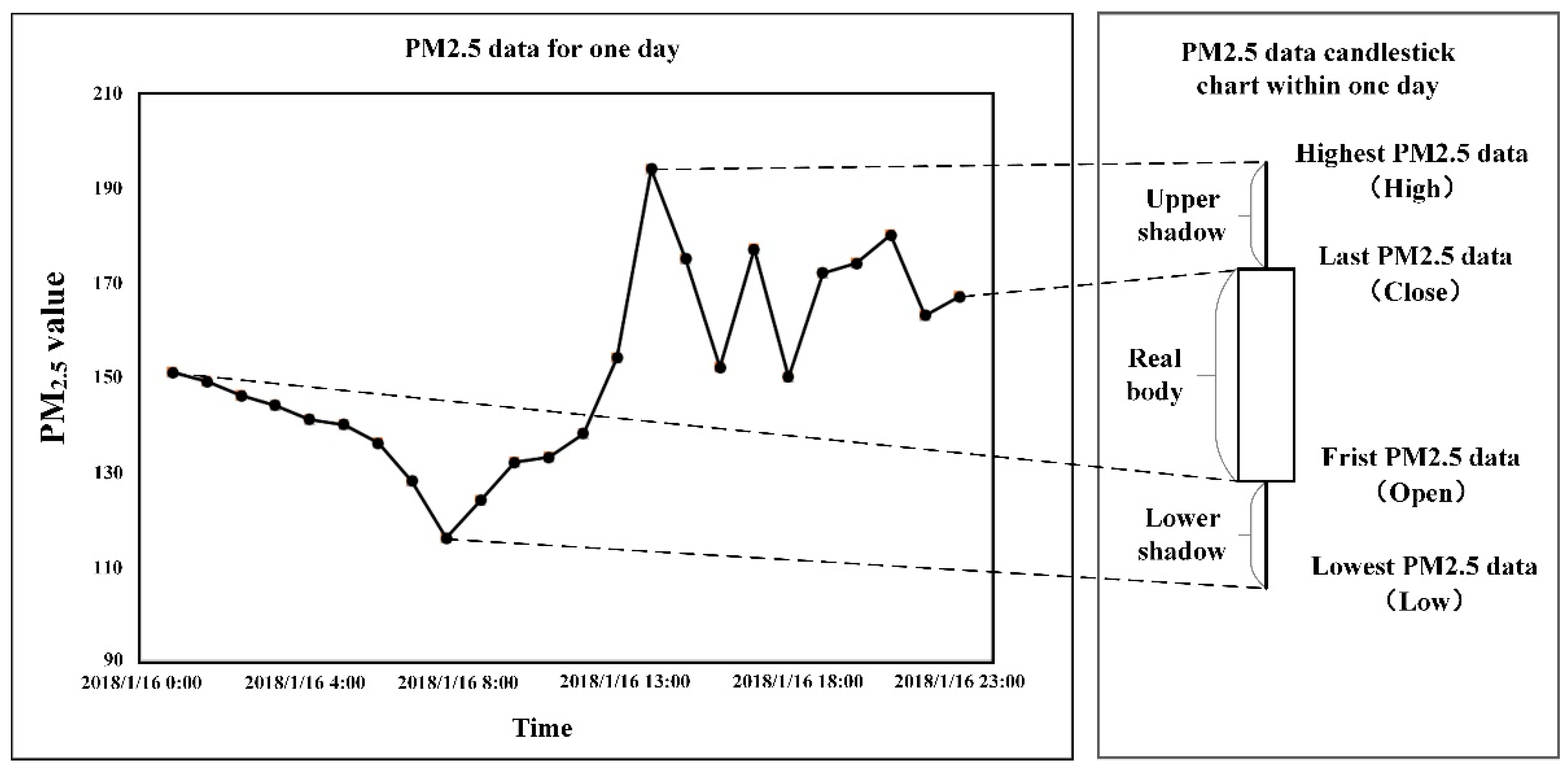
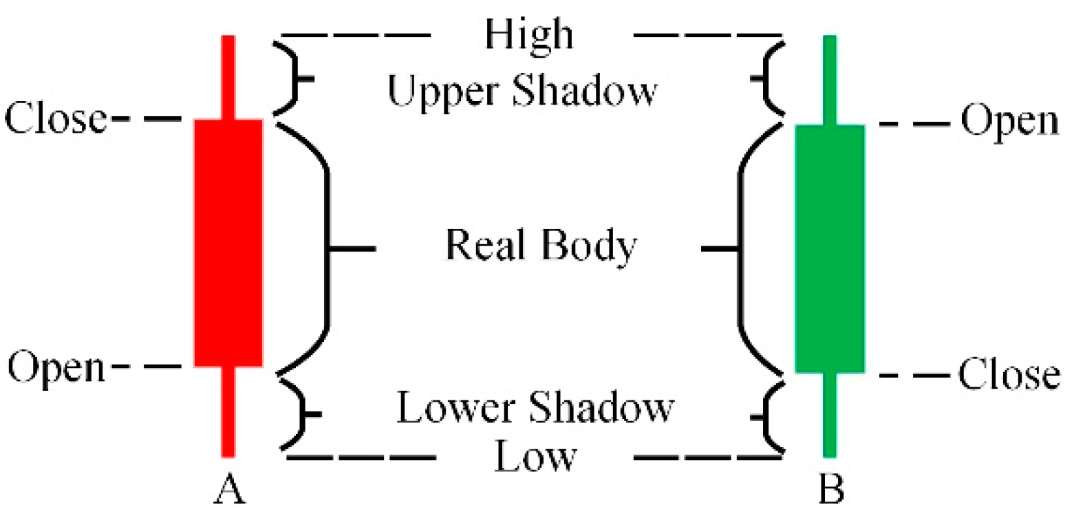
PM_2.5 data are typically time-series data, so it is feasible to predict future development using the past trend of PM_2.5 data. The candlestick chart was originally used to represent changes in stock prices over time [33,34,35,36]. It is a graph composed of stock data for multiple consecutive periods that can accurately reflect the four eigenvalues and the change process of stocks during a period [37,38,39]. Many scholars have used the candlestick chart to extract temporal features for trend predictions [40,41,42]. For example, the adaptive neuro-fuzzy inference system (ANFIS) is used to predict the stock market, which was constructed using the candlestick chart and imperial competitive algorithm (ICA) technology [43]. A method based on the candlestick chart to predict the change in adolescent stress levels was proposed that used the trend in the candlestick chart to reflect the trend in adolescent stress [44]. A novel fuzzy recommendation system for stock market investors was presented, and it adopted fuzzy Japanese candlesticks and included the effect of currency devaluation in the forecast [45]. However, these applications did not study specific physical principles. Thus, for studying the direction of air pollution, the candlestick chart explained using the Gaussian diffusion model has physical meaning.

At present, these studies on PM_2.5 cannot fully reflect the physical principles of PM_2.5 transmission. This problem directly leads to the low accuracy of PM_2.5 forecasts. This study examines the use of extracting the candlestick chart characteristics to reflect the PM_2.5 diffusion characteristics. Therefore, a method for the candlestick chart characteristics to reflect the physical diffusion characteristics of PM_2.5 is proposed. The candlestick chart characteristics, which are consistent with the principle of continuous time physical transmission, are used to reflect the PM_2.5 physical diffusion characteristics. This technique will become a key to communicate the physical model and the statistical model, using candlestick chart features to reflect the features that affect PM_2.5 concentration in the Gaussian diffusion model. The VGG model that improves the convolutional neural network model (CNN) is used to classify the PM_2.5 data. This method proposes to solve the problem of the time series characteristics of the PM_2.5 data to connect the physical principles and deep statistical learning theory.

2. Problem Scenarios

2.1. The Candlestick Chart and the Gaussian Diffusion Equation

2.1.1. The Candlestick Chart

The Japanese candlestick chart was developed by Munehisa Homma during the 18th century and introduced to the Western world by Steve Nison in his book published in 1991 [46]. The candlestick chart is composed of an opening price, highest price, lowest price, and closing price. The color of the candlestick chart is determined by the opening price and the closing price. A green candlestick chart means that the closing price is higher than the opening price, and a red candlestick chart means that the closing price is lower than the opening price. For one day of PM_2.5 data, the initial value corresponds to the opening price, the end value corresponds to the closing price, the minimum value corresponds to the lowest price, and the maximum value corresponds to the highest price, as shown in Figure 1.

A red candlestick means that the end value is smaller than the initial value, indicating that the PM_2.5 concentration is decreasing. A green candlestick means that the end value is greater than the initial value, indicating that the PM_2.5 concentration is rising. In Figure 1, Open and Close in A and B are opposite, and Low and High are the same.

PM_2.5 exists as the initial, end, maximum, and minimum values in different periods, which vary regularly. The candlestick chart is made from these four characteristic values, and it is able to reflect the time-series variation regulation [47]. In the financial field, a candlestick chart is used based on perceptual cognition due to a lack of mechanism support. Therefore, a method for PM_2.5 data feature extraction and classification combined with the Gaussian diffusion model and candlestick chart was designed that will provide basic theoretical support for the extraction of pollution process features during the pollutant PM_2.5 data period.

2.1.2. The Gaussian Diffusion Model and the Candlestick Chart

In the practical work of an atmospheric environmental impact assessment, Gaussian diffusion is typically used for the atmospheric diffusion calculation [48,49,50]. The Gaussian diffusion model is a point source diffusion model that is suitable for uniform atmospheric conditions and an area of wide and flat ground [51]. It can be used to discuss the diffusion of PM_2.5. The specific equation is as follows:

$$X\left(x,y,z,t,H\right)=\frac{Q}{2\pi v{\sigma }_y{\sigma }_z}exp(-\frac{1}{2}\frac{y^2}{{\sigma }_y^2})\times (exp(-\frac{1}{2}\frac{{(z-H)}^2}{{\sigma }_z^2})+exp(-\frac{1}{2}\frac{{(z+H)}^2}{{\sigma }_z^2}))$$

(1)

where X (x, y, z, t, H) is the gas concentration (kg/m³) diffused x meters downwind, y meters laterally, and z meters above the ground; σ_x, σ_y, and σ_z (m) are the diffusion parameters on the x, y, and z axes, respectively, and calculated according to the atmospheric stability selection parameter; H (m) is the height of the monitoring point; and v (m/s) is the wind speed.

Without considering the spatial model, one-dimensional analysis of the PM_2.5 diffusion process between the stations was conducted in combination with the source intensity, wind direction, and wind speed. The site located in the upwind direction of the target site was regarded as the occurrence location of the PM_2.5. To simplify the target site upwind site as the birthplace of PM_2.5, it was referred to as the strong source. The Gaussian diffusion model was established to simulate the diffusion process of PM_2.5 and analyze the PM_2.5 of the target stations.

As shown in Figure 2, A, B, C, and D represent the four sites in the research area, with site C as the target site and site B as the PM_2.5 source site. Assuming that the wind direction was from site B to site C, the diffusion process from site B to site C is indicated by the arrow.

Supposing that only one-dimensional diffusion was considered in the simulation process, and Q is the concentration of PM_2.5 at the strong source, v is the wind speed, d is the wind direction, and the concentration of PM_2.5 at the target point C is equivalent to the concentration of gas X in the Gaussian diffusion model. When the PM_2.5 data of Site C was only affected by site B, the parameter sensitivity analysis combined with the Gaussian diffusion equation will result in the following three situations showed in Figure 3: When Q is unchanged, the relationship between the change in v and C, and the relationship between the change between d and C are shown in Figure 3a,b respectively. Moreover, when v and d remain unchanged, the relationship between Q and C is shown in Figure 3c.

Table 1. Nine basic patterns of the candlestick charts.

Candlestick Chart
Q	increases	Y	Y	Y	N	N	Y	Y	Y	N	N	N	N	N	N
	decreases	N	N	N	N	N	N	N	N	N	N	Y	Y	Y	N
d	increases	N	Y	Y	Y	Y	N	Y	Y	Y	Y	N	N	N	N
	decreases	N	N	N	N	N	N	N	N	N	N	N	Y	Y	Y
v	increases	N	N	Y	N	Y	N	N	Y	N	Y	N	N	N	N
	decreases	N	N	N	N	N	N	N	N	N	N	N	N	Y	N

shows the Gaussian process corresponding to the nine forms of the candlestick chart. Among them, the wind direction (d) is increased when the wind blows from the pollution source to the target site, and the wind direction (d) is decreased when there is no wind blowing from the pollution source to the target site. The wind speed (v) is increased when the wind speed from the pollution source increases, and the wind speed (v) is decreased when the wind speed from the pollution source decreases. Y represents that the item has changed, and N represents that the item has not changed.

The source intensity (Q), wind speed (v), and wind direction (d) extracted by the Gaussian equation directly affect the change of PM_2.5 concentration. These three variables are also related to the variables affecting stocks in the financial market. Among them, the source intensity (Q) corresponds to the trading volume of the stock, which has a direct and obvious impact on the stock. The wind speed (v) corresponds to the trading speed of the stock, which affects the stock index to some extent. The wind direction (d) corresponds to an increase or decrease in stock holdings, which directly determines the direction of the stock.

The PM_2.5 candlestick chart is composed of an initial value, an end value, a maximum value, and a minimum value. Among them, a red candlestick represents the overall downward trend of PM_2.5 concentration on this day. A green candlestick represents the overall increase in PM_2.5 concentration on this day. According to the four values of the initial value, end value, maximum value, and minimum value, the length of the upper shadow line, the lower shadow line, and the entity are confirmed. The nine basic forms of PM_2.5 candlestick charts are obtained from differences in the length and color of the upper and lower shadows and the entities.

Table 2. The calculation methods of the nine basic forms of PM_2.5 candlestick chart.

The PM2.5 Candlestick Chart	The Computed Mode
	MAX * = END * > INIT * = MIN *
	MAX > END > INIT = MIN
	MAX = END > INIT > MIN
	MAX > END > INIT > MIN
	MAX = END > INIT = MIN
	MAX = INIT > END = MIN
	MAX > INIT > END = MIN
	MAX = INIT > END > MIN
	MAX > INIT > END > MIN

* MAX is the maximum value, END is the end value, INIT is the initial value, MIN is the minimum value.

shows the calculation methods of the nine basic forms of PM_2.5 candlestick chart.

2.2. Data Sources

The data for the study came from the online monitoring stations of air quality in Guilin. Since the primary pollution in Guilin is from external sources, Guilin is an ideal source of data. Using the PM_2.5 data of Guilin City to reflect the relationship between the Gaussian diffusion model and the candlestick chart, this research was less affected by sudden changes. In addition, the transmission of PM_2.5 between the stations in Guilin City was regarded as a uniform atmospheric condition. The Guilin Monitoring Station was selected as the target site. The hourly PM_2.5 data from 2013 to 2018 was selected as the basic dataset, which included the six-year hourly PM_2.5 data of the station. Figure 4 shows the location of the target site.

3. Method

3.1. Technical Route

A method was designed to extract the transmission characteristics of sequential PM_2.5 using the candlestick chart. The six-year PM_2.5 hourly data of the Guilin Monitoring Station was used as the research data. First, the candlestick chart sample generator was designed to convert the PM_2.5 data into a three-day candlestick chart format. Then these candlestick charts were classified to find the possible combination types using unsupervised classification methods. In addition, the accuracy of the unsupervised classification was obtained by judging the change trend of the PM_2.5 concentration of each type during the next period. Finally, the candlestick chart marked with the classification labels was trained and classified using the VGG model. After the classification results were obtained, the classification accuracy of the VGG model was counted and compared with other classification models. The PM_2.5 data classification framework is shown in Figure 5.

3.2. Candlestick Chart Sample Generator

The real body of the candlestick is composed of the initial and end values of the PM_2.5 data for a 24-h day, as shown in Figure 6. The upper and lower shadows of the candlestick are formed by connecting the maximum and minimum of the PM_2.5 data for the 24-h day and the physical column by thin lines. As a result, the PM_2.5 data in the form of a candlestick chart is displayed.

Since PM_2.5 hourly data is used as basic research data, there are 24 values for one day of PM_2.5 data. The entity of the candlestick chart is composed of the initial value and the end value of the day. The maximum value of the candlestick chart is the highest value of PM_2.5 concentration in a day, and the minimum value of the candlestick chart is the lowest value of PM_2.5 concentration in a day. In this way, one day of PM_2.5 data is transformed into a candlestick chart.

The convolution principle was adopted by the candlestick chart sample generator. The PM_2.5 data formed a candlestick graph every three days by setting the sliding window size to three days and the sliding step to one day, as shown in Figure 7. A candlestick chart combination was formed using the three-day PM_2.5 data. In Figure 7, the time-series data is continuous PM_2.5 data in daily units, with 24 data per day. The candlestick chart sample generator only coevolved the sequence of time.

3.3. Candlestick Chart Unsupervised Classification and Evaluation

The candlestick chart image data classification here refers to the extraction and differentiation of the characteristics of the PM_2.5 transmission process. The candlestick chart underwent image processing and was analyzed using unsupervised classification, and then the results were evaluated.

In order to improve the accuracy of candlestick chart classification, it is necessary to determine the duration of PM_2.5 pollution, and use this to determine the duration of a candlestick chart combination. PM_2.5 data from January 2013, a period of severe pollution, were selected as the study object. Figure 8 shows a line chart of PM_2.5 data at the monitoring station in January 2013.

It can be seen from Figure 8 that the duration of PM_2.5 pollution that occurred during the selected time is three days. It can also be said that the value of PM_2.5 will reach its peak after three days from the beginning of PM_2.5 pollution. After verification with a large amount of data, it was found that the PM_2.5 pollution duration of the site was three days most of the time. After analysis, it was found that this was because the source intensity, Q, wind speed, v, and wind direction, d, are updated faster, so that the PM_2.5 pollution situation will be updated within three days. Therefore, it was most appropriate to judge the average change in the PM_2.5 concentration over the following three days. Formula (2) is a specific evaluation formula. At the same time, it is also determined that the duration of the next candlestick chart combination is three days.

$$Y=\frac{{{\displaystyle \sum }}_{i=1}^3{x}_i}{3}-\frac{{{\displaystyle \sum }}_{j=1}^3{x}_j}{3}$$

(2)

where Y represents the difference between the current three-day average PM_2.5 concentration and the next three-day average PM_2.5 concentration. When Y > 0, it means that the pollution will be reduced in the future; when Y < 0, it means that pollution will increase in the future. x_i is the current average PM_2.5 concentration on day i, and x_j is the average PM_2.5 concentration on day j in the future.

3.4. VGG Model

VGG is a network model proposed by the Oxford Visual Geometry Group that was adapted from the CNN model [52]. The improvement in the VGG model compared to the CNN model is that it uses several consecutive 3 × 3 convolution kernels to replace the larger convolution kernels of the CNN model. The VGG model replaces the large-scale convolution kernel by stacking multiple small convolution kernels, which reduce the training parameters while ensuring the same receptive field. In the convolutional layer, the calculation of the receptive field is as follows:

$$r_n=\left(r_{n+1}-1\right)S_n+k_n$$

(3)

where r_n is the size of the receptive field of this layer; k_n is the size of the convolution kernel of this layer; and S_n is the size of the convolution stride.

For the classification experiment of the PM_2.5 data in the form of a candlestick chart, a VGG model was designed that contained six fundamental hidden layers; namely, a convolutional layer, a pooling layer, a flattened layer, a fully connected layer, and two other functional layers (i.e., the flattened layer and the dropout layer), as shown in Figure 9.

The rectifying linear element (ReLU) was used as the activation function for all of the hidden layers in VGG model, which can effectively avoid the gradient disappearance problem. The max () function was used to describe the ReLU function, as shown in Equation (4):

$$f\left(x\right)=max\left(0, x\right)$$

(4)

The ReLU function is equivalent to nonlinear mapping, which can increase the expression capacity of the network. Each weight, $a_{j,}^i$ of the feature map can be calculated according to Equation (5):

$$a_j^i=f\left({{\displaystyle \sum }}_{i\in M_j}{w}_j^i{a}_i^{i-1}+b_j^i\right)$$

(5)

where $w_j^i$ represents the kernel weight of the jth feature graph at layer i, which connects all the feature graphs at layer i − 1. M_j represents all the feature graphs connected by the jth feature graph in layer i. Cross entropy is used as the cost function, which is defined as:

$$Loss=-\left[{{\displaystyle \sum }}_{i=1}^n{{\displaystyle \sum }}_{k=1}^3{\widehat{y}}_k^{\left(i\right)}log\left(y_k^{\left(i\right)}\right)\right]$$

(6)

where n is the number of training instances; ${\widehat{y}}_k^{\left(i\right)}$ is the ith training and an instance of the kth forecast results; and $y_k^{\left(i\right)}$ represents the kth true result of the ith training instance:

$$y_k^{\left(i\right)}=\frac{e^{{\theta }^{\left(k\right)T_x^{\left(i\right)}}}}{{{\displaystyle \sum }}_{j=1}^3{e}^{{\theta }^{\left(j\right)T_x^{\left(i\right)}}}}$$

(7)

4. Analysis of Results

4.1. Evaluation Index

To achieve the optimal hyper-parameter values, the performance of the VGG model was evaluated using two metrics: overall accuracy (OA) and the Kappa index [53,54,55].

OA refers to the proportion of correctly classified samples to all samples, and its calculation equation is:

$$OA=\frac{TP+TN}{TP+FN+FP+TN}$$

(8)

where TP is a positive sample that is correctly classified by the model; FN is a positive sample that is incorrectly classified by the model; FP is a negative sample that is incorrectly classified by the model; and TN is a negative sample that is correctly classified by the model.

The Kappa coefficient is a type of ratio that represents the ratio of the error reduction between classifications and a completely random classification. Its calculation equation is:

$$K=\frac{p_0-p_e}{1-p_e}$$

(9)

where p₀ is the sum of the number of samples correctly classified in each category divided by the total number of samples, which is OA. Supposing that the number of real samples in each category is a₁, a₂, …, a_c, the predicted number of samples in each category is b₁, b₂, …, b_c, and the total number of samples is N, then:

$$p_e=\frac{a_1\times b_1+a_2\times b_2+\dots +a_c\times b_c}{N^2}$$

(10)

4.2. Hyper Parameter Settings

To evaluate the performance of the VGG model, some hyperparameters need to be set. The primary parameters that need to be set are the default dimensions of the VGG model (m), the input size (s_i), the number of convolution kernels (n_c), the size of the convolution kernel (s_c), the size of the pooling window (s_p), and the number of dense units (n_d). The hyperparameter setting here adopts the hyperparameter setting of the CNN model in Suoyan Pan’s research [56].

Table 3. Hyper-parameters involved in the VGG model.

Hyper-Parameters	Initial Values
Default dimension of the VGG model (m)	2
Input size (si)	9
Number of convolution kernels (nc)	256
size of the convolution kernel (sc)	3
Pooling window size (sp)	2
Number of dense units (nd)	1024

shows the hyper-parameters in the VGG model.

4.3. Results and Analysis

4.3.1. Candlestick Chart Combination

After implementing unsupervised classification of 2188 groups of PM_2.5 data, from the Guilin Monitoring Station, in the form of a candlestick chart, 16 candlestick chart combinations were obtained. Using Equation (2) as the evaluation index, the accurate data of future change trend prediction reached 99.68%, which was verified using the PM_2.5 data of the site from 2013 to 2018. It showed that the future change trend of PM_2.5 was accurately obtained using these 16 candlestick chart combinations, as shown in

Table 4. Eight categories of the candlestick chart combinations for PM_2.5 increases.

Species	1	2	3	4	5	6	7	8
Candlestick chart
Q increases	Y	N	N	Y	N	N	Y	Y
v increases	N	Y	Y	N	N	N	N	N
d changes	N	N	N	N	Y	Y	N	N
Number of samples (%)	6.21	5.94	5.85	5.25	7.04	6.67	6.17	5.62
Accuracy (%)	99.96	99.28	99.89	99.18	98.86	100	99.69	99.89

and

Table 5. Eight categories of the candlestick chart combinations for PM_2.5 declines.

Species	9	10	11	12	13	14	15	16
Candlestick chart
Q decreases	Y	N	N	Y	Y	N	N	Y
v decreases	N	Y	Y	N	N	N	N	N
d changes	N	N	N	N	N	Y	Y	N
Number of samples (%)	6.12	6.72	6.12	5.71	6.76	7.17	7.04	5.62
Accuracy (%)	99.87	99.67	99.88	99.83	99.73	99.28	99.97	99.89

.

In Table 4 and Table 5, the 16 candlestick chart combinations are listed. Among them, eight combinations predicted that the future PM_2.5 concentration will increase, and eight combinations predicted that the future PM_2.5 concentration will decrease. It also lists the corresponding relationship between the 16 combinations that will cause changes in the PM_2.5 concentration in the following days, the parameter changes in the Gaussian equation, and the proportion of each category to the total number of samples. In Table 4 and Table 5, Y represents that the item has changed, and N represents that the item has not changed. As Guilin is a low-industry city, the primary form of pollution is from external pollution sources. Hence, the 16 changes in the figure below will not appear when the source strength, Q, wind speed, v, and wind direction, d, do not change.

The 16 candlestick chart combinations shown in Table 4 and Table 5 reflect the 16 kinds of PM_2.5 characteristics of change. There are three main variables affecting the change of PM_2.5 concentration, namely source intensity (Q), wind speed (v), and wind direction (d). Among them, the source intensity (Q) represents the total pollution of PM_2.5, which will have a direct impact on the change of PM_2.5 concentration. When the Q increases, the PM_2.5 concentration will increase significantly in the future, which will lead to the occurrence of combinations 1, 4, 7, and 8. When the Q decreases, the PM_2.5 concentration will decrease significantly in the future, which will lead to the occurrence of combinations 9, 12, 13, and 16. The wind speed (v) represents the pollution rate of PM_2.5, which determines the change rate of PM_2.5 concentration. When the v increases, there will be a significant increase in PM_2.5 concentration in the future, which will lead to combinations 2 and 3. When the v decreases, the PM_2.5 concentration will decrease significantly in the future, which will lead to the occurrence of combinations 10 and 11. The wind direction (d) determines the change state of PM_2.5. When the d changes, it will directly lead to the color change of PM_2.5 candlestick diagram, thus affecting the future PM_2.5 concentration change. Combinations 5, 6, 14, and 15 are due to the change of d to determine the future trend of PM_2.5 concentration.

Hu et al. proposed 103 candlestick chart combinations in 2019, of which there were 29 candlestick chart combinations for three days [57]. By examining the comparison, it was found that in the 16 candlestick chart combinations obtained by the unsupervised classification, all of them matched these 29 three-day candlestick chart combinations. There were only 16 candlestick chart combinations at the Guilin Monitoring Station because the PM_2.5 pollution types in Guilin are primarily from external pollution sources, while the unmatched types primarily occur under self-pollution.

4.3.2. Analysis of the VGG Model Classification Results

All the deep learning models in this research were trained on TensorFlow, and the traditional machine learning models were implemented through the scikit-learn library, and RMSprop was used as the optimizer.

The Guilin Monitoring Station was selected as the target site, and the PM_2.5 data in the form of a candlestick chart for the six years from 2013 to 2018 was used as the basic dataset. The four-year candlestick chart PM_2.5 data from 2013 to 2016 was used as the training set, and the two-year data from 2017 and 2018 was used as the test set. After training and convergence, the optimal model weights of the six hyperparameters of the VGG classification model were obtained, namely m = 2, s_i = 9, n_c = 256, s_c = 3, s_p = 2, and n_d = 1024. The number of each category and OA value after classification are shown in

Table 6. The numbers and accuracies of the data classification samples.

Category	Number of Samples	Number of Classifications	OA (%)	Average Accuracy (%)
1	136	132	97.06	96.19
2	130	125	96.15
3	128	123	96.09
4	115	110	95.65
5	153	146	95.42
6	146	141	96.58
7	135	127	94.07
8	123	119	96.75
9	134	130	97.01
10	147	142	96.60
11	134	129	97.76
12	125	122	95.20
13	148	141	95.27
14	157	152	96.82
15	154	149	96.75
16	123	118	95.93

.

It can be seen from Table 6 that the total number of samples was 2188, and the average accuracy of each category reached 96.19%. The number of samples in the 16 categories was close to the number of samples in each category in Table 4 and Table 5. This indicates the accuracy of the definition of the 16 candlestick chart combinations. It further indicates the feasibility of using the candlestick chart to reflect the physical diffusion characteristics of PM_2.5.

The confusion matrix, also known as the error matrix, is a standard format for accuracy evaluation that can reflect the accuracy of the image classification. The VGG model classification results displayed by the confusion matrix are shown in Figure 10. In Figure 10, the size of the value is represented by the square size and color depth. The Kappa coefficient of the VGG model classification experiment calculated by the confusion matrix was 0.960. According to the calculation result of the Kappa coefficient, it is known that the classification accuracy of the VGG model is very high using the candlestick chart feature to reflect the physical diffusion feature of PM_2.5.

4.3.3. Model Comparison Analysis

To verify the classification performance of the VGG model, the VGG model was compared with three models, SVM, LeNet, and AlexNet, using the OA, Kappa values, and training times as quantitative results, as shown in

Table 7. A comparison of the four classification models for the classification accuracies and time complexities.

Model	OA (%)	Kappa	Time (mins)
SVM	92.83	0.916	786
LeNet	94.41	0.935	1005
AlexNet	95.68	0.946	1124
VGG	96.19	0.960	530
Improvements	1.93	0.03	442

.

It can be seen from Table 7 that the OA, Kappa values, and training times of the VGG model were the best of all the experimental models. Comparatively, the VGG model had the least computational burden because the model contained only six fundamental function layers, rather than the deeper and repetitive functional layers. Using a comparison, it was found that the VGG model with the best hyperparameters had the highest classification accuracy, with the OA and Kappa values improved by approximately 0.56–3.41% and 0.01–0.044, respectively.

Figure 11 shows a candlestick chart of the PM_2.5 data conversion during the first and fourth quarters of 2018. By utilizing the classification results of PM_2.5 data from the first two weeks of January 2018 as an example, the graphical displays of classification results of the four models are shown in Figure 12. Marks 1–8 in Figure 12 refers to the classification of the future PM_2.5 concentration increases, and marks 9–16 refer to the classification of the future PM_2.5 concentration decreases. Referring to Table 4 and Table 5, the classification results of the four models of the SVM, LeNet, AlexNet, and VGG, which intercepted some data, were judged based on actual data. It was found that the accuracy of the classification results of the VGG model reached 100%, as shown in Figure 12a. Therefore, the VGG model accurately classified all of the PM_2.5 data. However, the other three models had classification errors, and the errors all appeared between similar categories. The 8th category was incorrectly classified into the 12th category by the SVM model, as shown in Figure 12b. The 10th category was incorrectly classified into the 4th category by the LeNet model, as shown in Figure 12c. The 13th category was incorrectly classified by the AlexNet model divided into the third category, as shown in Figure 12d.

This was mainly because (1) the VGG model primarily contained fundamental function layers, which guaranteed the classification accuracies by using the PM_2.5 data in the form of a candlestick chart; and (2) the VGG model was not encumbered by a large number of implementation layers, which greatly shortened the model training time to improve the PM_2.5 data classification efficiency.

5. Conclusions and Prospects

The physical principle of PM_2.5 transmission has not been reflected by current studies that have examined PM_2.5 transmission simulations. This is because the machine learning models and hybrid models used by these studies were black-box models. These black-box models are established based on the relationship between input and output. Although this reflects a general direct causal relationship between related factors, it cannot describe the specific physical process and lacks data on periodic characteristics. Therefore, a method was proposed to reflect the physical diffusion characteristics of PM_2.5 using the candlestick chart characteristics. After implementing unsupervised classification on 2188 groups of PM_2.5 data in the form of a candlestick chart from the Guilin Monitoring Station, 16 candlestick chart combinations were obtained. Using the average concentration change of PM_2.5 in the next three days as the evaluation index, the accurate data for predicting the future change trend reached 99.68%, which was verified by the PM_2.5 data of the site from 2013 to 2018. The candlestick chart feature that conformed to the physical transmission principle of the continuous period was extracted using the VGG model of the deformed conventional neural network model (CNN). These characteristics reflected the physical diffusion characteristics of PM_2.5. Additionally, the classification accuracy of the PM_2.5 data classification was improved using this method.

In the experimental verification portion, the performance of the model was evaluated and compared with the SVM, LeNet, and AlexNet models. The experimental results showed that the overall accuracy (OA) value of the candlestick chart combination classification was 96.19%, and the Kappa coefficient was 0.960. Compared with the support vector machines (SVM), LeNet, and AlexNet models, the overall accuracy of the VGG model was improved by 1.93% on average. It shows that the PM_2.5 data was effectively classified using this method, and the VGG model combined with the candlestick chart was more accurate than the other classification models. In addition, the problem of connecting the physical mechanism and statistical theory using the time series characteristics of the PM_2.5 transmission was solved.

Guilin City was used as the research area during the research process. Therefore, the 16 candlestick chart combinations proposed are only applicable to the PM_2.5 studies in this region, and their applicability to other regions remains to be verified. In addition, the method proposed by this study can only predict the PM_2.5 change trend for the next three days, and an accurate predicted value of PM_2.5 will be proposed in future research.

During the transmission of atmospheric pollutants, the transmission of PM_2.5 is affected by factors such as temperature inversions, the natural environment, and human activities. By considering the atmospheric transmission trajectory, local atmospheric turbulence, and human activities, the area represented by the site, which is the regional center, was constructed using the equivalent distance weight method according to the terrain and vegetation. In addition, endogenous and exogenous pollution in the study area were also considered, and by using the backward air mass trajectory and the occurrence of a temperature inversion, a hybrid model of the VGG model based on the candlestick chart and the long and short-term memory network time cycle neural network (LSTM) was constructed. This technique is a more accurate research method to predict the specific value of PM_2.5.

References

1. Wang, Y.; Shi, L.; Lee, M.; Liu, P.; Di, Q.; Zanobetti, A.; Schwartz, J.D. Long-term Exposure to PM2.5 and Mortality Among Older Adults in the Southeastern US. Epidemiology 2016, 28, 207. [Google Scholar] [CrossRef] [PubMed]
2. Li, C.Y.; Wu, C.D.; Pan, W.C.; Chen, Y.C.; Su, H.J. Association Between Long-term Exposure to PM2.5 and Incidence of Type 2 Diabetes in Taiwan: A National Retrospective Cohort Study. Epidemiology 2019, 30 (Suppl. 1), S67–S75. [Google Scholar] [CrossRef]
3. Wang, F.; Qiu, X.; Cao, J.; Peng, L.; Zhang, N.; Yan, Y.; Li, R. Policy-driven changes in the health risk of PM2.5 and O3 exposure in China during 2013–2018. Sci. Total Environ. 2021, 2021, 757. [Google Scholar]
4. Nursan, C.; Alvur, T.M.; Cemile, D.; Pinar, T.; Sevin, A. Parent’s knowledge and perceptions of the health effects of environmental hazards in Sakarya, Turkey. J. Pak. Med. Assoc. 2014, 64, 38. [Google Scholar] [PubMed]
5. Xiaoqi, W.; Wei, W.; Shuiyuan, C.; Jianbing, L. Characteristics and classification of PM2.5 pollution episodes in Beijing from 2013 to 2015. Sci. Total Environ. 2017, 612, 170–179. [Google Scholar]
6. Byun, D.; Schere, K.L. Review of the governing equations, computational algorithms, and other components of the Model-3 Community Multiscale Air Quality (CMAQ) modeling system. Appl. Mech. Rev. 2006, 59, 51–77. [Google Scholar] [CrossRef]
7. Zhou, Q.; Jiang, H.; Wang, J.; Zhou, J. A hybrid model for PM 2.5 forecasting based on ensemble empirical mode decomposition and a general regression neural network. Sci. Total Environ. 2014, 496, 264–274. [Google Scholar] [CrossRef]
8. Wang, Z.; Guo, L.; Han, D.; Gu, F. An ultrasensitive calcein sensor based on the implementation of a novel chemiluminescence system with modified kaolin. Sens. Actuators B Chem. 2015, 212, 264–272. [Google Scholar] [CrossRef]
9. Zhai, B.; Chen, J. Development of a stacked ensemble model for forecasting and analyzing daily average PM 2.5 concentrations in Beijing, China. Sci. Total Environ. 2018, 635, 644–658. [Google Scholar] [CrossRef]
10. Hu, H.; Dailey, A.B.; Kan, H.; Xu, X. The effect of atmospheric particulate matter on survival of breast cancer among US females. Breast Cancer Res. Treat. 2013, 139, 217–226. [Google Scholar] [CrossRef]
11. Chemel, C.; Fisher, B.E.A.; Kong, X.; Francis, X.V.; Sokhi, R.; Good, N.; Collins, W.; Folberth, G. Application of chemical transport model CMAQ to policy decisions regarding PM2.5 in the UK. Atmos. Environ. 2014, 82, 410–417. [Google Scholar] [CrossRef] [Green Version]
12. Djalalova, I.; Delle Monache, L.; Wilczak, J. PM2.5 analog forecast and Kalman filter post-processing for the Community Multiscale Air Quality (CMAQ) model—ScienceDirect. Atmos. Environ. 2015, 108, 76–87. [Google Scholar] [CrossRef]
13. Sugimoto, N.; Shimizu, A.; Matsui, I.; Nishikawa, M. A method for estimating the fraction of mineral dust in particulate matter using PM2.5-to-PM10 ratios. Particuology 2016, 28, 114–120. [Google Scholar] [CrossRef]
14. Sun, W.; Zhang, H.; Palazoglu, A.; Singh, A.; Zhang, W.; Liu, S. Prediction of 24-hour-average PM2.5 concentrations using a hidden Markov model with different emission distributions in Northern California. Sci. Total Environ. 2013, 443, 93–103. [Google Scholar] [CrossRef] [PubMed]
15. Mishra, D.; Goyal, P.; Upadhyay, A. Artificial intelligence based approach to forecast PM2.5 during haze episodes: A case study of Delhi, India. Atmos. Environ. 2015, 102, 239–248. [Google Scholar] [CrossRef]
16. Yang, W.; Deng, M.; Xu, F.; Wang, H. Prediction of hourly PM 2.5 using a space-time support vector regression model. Atmos. Environ. 2018, 181, 12–19. [Google Scholar] [CrossRef]
17. Feng, X.; Fu, T.-M.; Cao, H.; Tian, H.; Fan, Q.; Chen, X. Neural network predictions of pollutant emissions from open burning of crop residues: Application to air quality forecasts in southern China. Atmos. Environ. 2019, 204, 22–31. [Google Scholar] [CrossRef]
18. Cheng, Y.; Zhang, H.; Liu, Z.; Chen, L.; Wang, P. Hybrid algorithm for short-term forecasting of PM 2.5 in China. Atmos. Environ. 2019, 200, 264–279. [Google Scholar] [CrossRef]
19. Liu, H.; Duan, Z.; Chen, C. A hybrid framework for forecasting PM2.5 concentrations using multi-step deterministic and probabilistic strategy. Air Qual. Atmos. Health 2019, 12, 785–795. [Google Scholar] [CrossRef]
20. Wu, H.; Liu, H.; Duan, Z. PM2.5 concentrations forecasting using a new multi-objective feature selection and ensemble framework. Atmos. Pollut. Res. 2020, 11, 1187–1198. [Google Scholar] [CrossRef]
21. Du, P.; Wang, J.; Hao, Y.; Niu, T.; Yang, W. A novel hybrid model based on multi-objective Harris hawks optimization algorithm for daily PM2.5 and PM10 forecasting. Appl. Soft Comp. 2020, 96, 106620. [Google Scholar] [CrossRef]
22. Sun, W.; Sun, J. Daily PM2.5 concentration prediction based on principal component analysis and LSSVM optimized by cuckoo search algorithm. J. Environ. Manag. 2016, 188, 144. [Google Scholar] [CrossRef] [PubMed]
23. Jiang, P.; Dong, Q.; Li, P. A novel hybrid strategy for PM2.5 concentration analysis and prediction. J. Environ. Manag. 2017, 196, 443–457. [Google Scholar] [CrossRef]
24. Mahajan, S.; Liu, H.M.; Tsai, T.C.; Chen, L.J. Improving the Accuracy and Efficiency of PM2.5 Forecast Service Using Cluster-Based Hybrid Neural Network Model. IEEE Access 2018, 6, 1. [Google Scholar] [CrossRef]
25. Liu, H.; Chen, C. Prediction of outdoor PM2.5 concentrations based on a three-stage hybrid neural network model. Atmos. Pollut. Res. 2019, 11, 469–481. [Google Scholar] [CrossRef]
26. Li, T.; Hua, M.; Wu, X. A Hybrid CNN-LSTM Model for Forecasting Particulate Matter (PM2.5). IEEE Access 2020, 8, 1. [Google Scholar] [CrossRef]
27. Nath, P.; Saha, P.; Middya, A.I.; Roy, S. Long-term time-series pollution forecast using statistical and deep learning methods. Neural Comput. Appl. 2021, 1–3. [Google Scholar] [CrossRef]
28. Kow, P.-Y.; Wang, Y.-S.; Zhou, Y.; Kao, I.-F.; Issermann, M.; Chang, L.-C.; Chang, F.-J. Seamless integration of convolutional and back-propagation neural networks for regional multi-step-ahead PM2.5 forecasting. J. Clean. Prod. 2020, 261, 121285. [Google Scholar] [CrossRef]
29. Feng, R.; Zheng, H.-J.; Gao, H.; Zhang, A.-R.; Huang, C.; Zhang, J.-X.; Luo, K.; Fan, J.-R. Recurrent Neural Network and random forest for analysis and accurate forecast of atmospheric pollutants: A case study in Hangzhou, China. J. Clean. Prod. 2019, 231, 1005–1015. [Google Scholar] [CrossRef]
30. Wang, Y.S.; Chang, L.C.; Chang, F.J. Explore Regional PM2.5 Features and Compositions Causing Health Effects in Taiwan. Environ. Manag. 2020, 67, 1–6. [Google Scholar] [CrossRef]
31. Chang, F.-J.; Chang, L.-C.; Kang, C.-C.; Wang, Y.-S.; Huang, A. Explore spatio-temporal PM2.5 features in northern Taiwan using machine learning techniques. Sci. Total Environ. 2020, 736, 139656. [Google Scholar] [CrossRef]
32. Minguillón, M.C.; Querol, X.; Baltensperger, U.; Prévôt, A.S.H. Fine and coarse PM composition and sources in rural and urban sites in Switzerland: Local or regional pollution? Sci. Total Environ. 2012, 427–428, 191–202. [Google Scholar] [CrossRef] [PubMed]
33. Xie, H.; Zhao, X.; Wang, S. A Comprehensive Look at the Predictive Information in Japanese Candlestick. Procedia Comput. Sci. 2012, 9, 1219–1227. [Google Scholar] [CrossRef] [Green Version]
34. Yuen, R.W.P. High Low Candlestick Chart. SSRN Electron. J. 2013. [Google Scholar] [CrossRef]
35. Lu, T.H. The profitability of candlestick charting in the Taiwan stock market. Pac. Basin Financ. J. 2014, 26, 65–78. [Google Scholar] [CrossRef]
36. Velez, O.L. The Japanese candlestick char. In Swing Trading, 3rd ed.; John Wiley & Sons, Inc.: Hoboken, NJ, USA, 2012; pp. 25–34. [Google Scholar] [CrossRef]
37. Lan, Q.; Zhang, D.; Xiong, L. Reversal Pattern Discovery in Financial Time Series Based on Fuzzy Candlestick Lines. Syst. Eng. Procedia 2011, 2, 182–190. [Google Scholar] [CrossRef] [Green Version]
38. Tsai, C.F.; Quan, Z.Y. Stock Prediction by Searching for Similarities in Candlestick Charts. ACM. TMIS 2014, 5, 1–21. [Google Scholar] [CrossRef]
39. Lu, T.H.; Chen, Y.C.; Hsu, Y.C. Trend definition or holding strategy: What determines the profitability of candlestick charting? J. Bank. Financ. 2015, 61, 172–183. [Google Scholar] [CrossRef]
40. Lee, K.H.; Jo, G.S. Expert system for predicting stock market timing using a candlestick chart. Expert Syst. Appl. 1999, 16, 357–364. [Google Scholar] [CrossRef]
41. Chen, S.; Bao, S.; Zhou, Y. The predictive power of Japanese candlestick charting in Chinese stock market. Phys. A Stat. Mech. Appl. 2016, 457, 148–165. [Google Scholar] [CrossRef]
42. Ni, Y.; Cheng, Y.; Huang, P.; Day, M.Y. Trading strategies in terms of continuous rising (falling) prices or continuous bullish (bearish) candlesticks emitted. Phys. A Stat. Mech. Appl. 2018, 501, 188–204. [Google Scholar] [CrossRef]
43. Barak, S.; Dahooie, J.H.; Tichy, T. Wrapper ANFIS-ICA method to do stock market timing and feature selection on the basis of Japanese Candlestick. Expert Syst. Appl. 2015, 42, 9221–9235. [Google Scholar] [CrossRef] [Green Version]
44. Li, Y.; Feng, Z.; Feng, L. Using Candlestick Charts to Predict Adolescent Stress Trend on Micro-blog. Procedia Comput. Sci. 2015, 63, 221–228. [Google Scholar] [CrossRef] [Green Version]
45. Naranjo, R.; Santos, M. A fuzzy decision system for money investment in stock markets based on fuzzy candlesticks pattern recognition. Expert Syst. Appl. 2019, 133, 34–48. [Google Scholar] [CrossRef]
46. Nison, S. Japanese Candlestick Charting Techniques; New York Institute of Finance: New York, NY, USA, 1991. [Google Scholar]
47. Marszałek, A.; Burczyński, T. Modeling and forecasting financial time series with ordered fuzzy candlesticks. Inf. Sci. 2014, 273, 144–155. [Google Scholar] [CrossRef]
48. Yook, S.J.; Ahn, K.H. Gaussian diffusion sphere model to predict mass transfer due to diffusional particle deposition on a flat surface in laminar flow regime. Appl. Phys. Lett. 2009, 94, 215. [Google Scholar] [CrossRef]
49. Duysebekova, K.; Serbin, V.; Kuandykov, A.; Duysebekov, T.; Alimanova, M.; Orazbekov, S.; Alimzhanova, L. The Solution of Semi-empirical Equation of Turbulent Diffusion in Problems of Polluting Impurity Transfer by Gauss Approach. Procedia Comput. Sci. 2016, 94, 372–379. [Google Scholar] [CrossRef] [Green Version]
50. Ye, W.; Zhou, B.; Tu, Z.; Xiao, X.; Yan, J.; Wu, T.; Tittel, F.K. Leakage source location based on Gaussian plume diffusion model using a near-infrared sensor. Infrared Phys. Technol. 2020, 109, 103411. [Google Scholar] [CrossRef]
51. Ichikawa, Y.; Shikata, H.; Nishinomiya, S. A Gaussian Trajectory Atmospheric Diffusion Model for Complex Terrain. J. Jpn. Soc. Atmos. Environ. 2011, 21, 104–114. [Google Scholar]
52. Simonyan, K.; Zisserman, A. Very Deep Convolutional Networks for Large-Scale Image Recognition. arXiv 2014, arXiv:1409.1556. [Google Scholar]
53. Congalton, R.G. A review of assessing the accuracy of classifications of remotely sensed data. Remote Sens. Environ. 1991, 37, 270–279. [Google Scholar] [CrossRef]
54. Holtz, T.S.U. Introductory Digital Image Processing: A Remote Sensing Perspective, 3rd ed. Environ. Eng. Geosci. 2007, 13, 89–90. [Google Scholar] [CrossRef]
55. Foody, G. Assessing the Accuracy of Remotely Sensed Data: Principles and Practices. Photogramm. Rec. 2010, 25, 204–205. [Google Scholar] [CrossRef]
56. Pan, S.; Guan, H.; Chen, Y.; Yu, Y.; Gonçalves, W.N.; Junior, J.M.; Li, J. Land-cover classification of multispectral LiDAR data using CNN with optimized hyper-parameters. ISPRS J. Photogramm. Remote Sens. 2020, 166, 241–254. [Google Scholar] [CrossRef]
57. Hu, W.; Si, Y.-W.; Fong, S.; Lau, R.Y.K. A formal approach to candlestick pattern classification in financial time series. Appl. Soft Comput. J. 2019, 84, 10570. [Google Scholar] [CrossRef]
Figure 1. Schematic diagram of Japanese Candlestick.
Atmosphere 12 00570 g001
Figure 2. The schematic diagram of the monitoring site location.
Atmosphere 12 00570 g002
Figure 3. Relationship between the PM2.5 concentration change at the target point. Assuming that Q is unchanged, the relationship between the change in v and C is shown in (a). Assuming that Q is unchanged, the relationship between the change in d and C is shown in (b). Assuming that v and d remain unchanged, the relationship between Q and C is shown in (c).
Atmosphere 12 00570 g003
Figure 4. Coordinate location map of the Guilin Monitoring station.
Atmosphere 12 00570 g004
Figure 5. PM2.5 data classification framework.
Atmosphere 12 00570 g005
Figure 6. A PM2.5 value candlestick chart within a day.
Atmosphere 12 00570 g006
Figure 7. Principle of the candlestick chart sample generator.
Atmosphere 12 00570 g007
Figure 8. Line graph of PM2.5 data at monitoring stations in January 2013.
Atmosphere 12 00570 g008
Figure 9. Architecture of the constructed VGG model.
Atmosphere 12 00570 g009
Figure 10. VGG classification results displayed in the confusion matrix.
Atmosphere 12 00570 g010
Figure 11. Candlestick chart of the PM2.5 data in 2018.
Atmosphere 12 00570 g011
Figure 12. Partial classification results of the VGG models, (a) VGG, (b) SVM, (c) LeNet, and (d) AlexNet.
Atmosphere 12 00570 g012