Abstract
Fine particulate matter (PM2.5) has a serious impact on human health. Forecasting PM2.5 levels and analyzing the pollution sources of PM2.5 are of great significance. In this study, the Lagrangian particle dispersion (LPD) model was developed by combining the FLEXPART model and the Bayesian inventory optimization method. The LPD model has the capacity for real-time forecasting and determination of pollution sources of PM2.5, which refers to the contribution ratio and spatial distribution of each type of pollution (industry, power, residential, and transportation). In this study, we applied the LPD model to the Beijing-Tianjin-Hebei (BTH) region to optimize the a priori PM2.5 emission inventory estimates during 15–20 March 2018. The results show that (1) the a priori estimates have a certain degree of overestimation compared with the a posteriori flux of PM2.5 for most areas of BTH; (2) after optimization, the correlation coefficient (R) between the forecasted and observed PM2.5 concentration increased by an average of approximately 10%, the root mean square error (RMSE) decreased by 30%, and the IOA (index of agreement) index increased by 16% at four observation sites (Aotizhongxin_Beijing, Beichenkejiyuanqu_Tianjin, Dahuoquan_Xintai, and Renmingongyuan_Zhangjiakou); and (3) the main sources of pollution at the four sites mainly originated from industrial and residential emissions, while power factory and transportation pollution accounted for only a small proportion. The concentration of PM2.5 forecasts and pollution sources in each type of analysis can be used as corresponding reference information for environmental governance and protection of public health.
1. Introduction
Over the past several decades, industrialization and urbanization have caused serious PM2.5 pollution in China. PM2.5 refers to atmospheric particulates with aerodynamic diameters less than 2.5 μm in ambient air [1,2]. Ambient particles can affect air quality and climate by absorbing and scattering solar irradiation [3,4,5,6], and they also have adverse effects on human health. Studies have shown that high concentrations of PM2.5 not only increase the morbidity and mortality of the public but also affect the cardiovascular system [7,8,9,10]. PM2.5 is more harmful to human health than PM10 because PM2.5 has a smaller particle size and a larger specific surface area, which makes it easier to absorb toxic chemicals [11,12]. Therefore, increasing attention has been given to PM2.5 in China, not only from the scientific community but also from the public. Overall, it is particularly important to accurately predict the PM2.5 concentration. In addition, to reduce PM2.5 concentrations, it is essential to understand the relative contributions to PM2.5 from various sources, and effective management and control strategies can only be developed for major emission sources when this information is obtained.
Generally, environmental pollution prediction methods are divided into two categories: deterministic and statistical methods [13]. Deterministic methods use mathematical methods to approximate the physical-chemical mechanisms of reaction, transport, and deposition processes to predict the concentration of pollutants. Using the atmospheric model to simulate PM2.5 for predicting air quality is a hot research topic at present. For example, the WRF-Chem and CMAQ models have been used to evaluate the responses of the surface PM2.5 level to emission mitigation. Because the model structure and parameter estimation are excessively dependent on ideal theoretical assumptions and large databases, the nonlinearity and heterogeneity of multiple factors cannot be well evaluated by the deterministic method [11,14]. With the continuous improvement in the air quality detection network and the continuous increase in the hourly concentration monitoring data of various pollutants, it is more convenient to use statistical methods to predict regional air quality. Huang et al., (2021) developed an integration method of gated recurrent unit neural networks based on empirical mode decomposition (EMD-GRU) for predicting PM2.5 concentrations [15]. Wen et al., (2019) constructed a convolutional long short-term neural network to predict the PM2.5 concentration in Beijing [16]. Zhu et al., (2021) proposed an attention-based parallel network (APNet) to predict PM2.5 concentrations in the subsequent 72 h [17]. There are also multiple linear regressions (MLRs) [18,19,20], neural networks (NNs) [21,22], fuzzy logic (FL) [23], autoregressive moving averages (ARIMAs) [24,25], machine learning (ML) [11,26,27,28,29], graph convolutional networks, and long short-term memory networks (GC-LSTMs) [30]. Compared with deterministic methods, statistical methods have the advantages of higher operational and simple model structure settings. In addition, related research shows that statistical methods have better forecasting effects than deterministic methods [31,32].
Effective management and control strategies rely on high-precision pollutant forecasts; however, these strategies also need to fully understand the emission sources of pollutants. Qie et al., (2018) used the principal component analysis (PCA) method combined with the Hybrid Single-Particle Lagrangian Integrated Trajectory (HYSPLIT) model and potential source contribution function (PSCF) to analyze the distribution and sources of PM2.5 [33,34]. Caili et al., (2021) built a comprehensive framework based on a horizontal 2-dimensional transport model to optimally estimate the initial concentrations and emission sources of PM2.5 with 4D-Var [35]. Guo et al., (2018) used the FLEXPART-WRF model combined with the Bayesian optimization method to retrieve and optimize the emission inventory of PM2.5 [36]. An emission database for global atmospheric research (EDGAR) was developed by scientists at the Netherlands Organization for Applied Scientific Research (TNO) and the National Institute for Public Health and the Environment (RIVM) [37]. Zhang et al., (2009) established an inventory of air pollutant emissions in Asia for 2006 to support the Intercontinental Chemical Transport Experiment-Phase B (INTEX-B) [38]. Yan et al., (2020) used the PMF (positive matrix factorization) model to analyze the main contribution source of PM2.5 when the AQI exceeds 200 in urban residential areas [39]. Fan et al., (2018) used diagnostic ratios to invert the source of PM2.5 pollution in Guiyang [40]. Hu et al., (2017) used the PCA method to study the main pollution sources in Hefei from 2014 to 2015 [41].
However, there are a few studies that simultaneously analyze the pollution sources during the process of pollutant forecasting, which can help clearly understand the pollution source distribution during a pollution process and propose targeted solutions. Therefore, the main objective of this study is to develop an LPD (i.e., the FLEXPART model combined with the Bayesian method) model for real-time forecasting of PM2.5 concentrations and emission source analysis. In this model, to improve the hourly prediction accuracy of PM2.5, the Bayesian optimization method was used to calibrate the monthly inventory of PM2.5 emissions and to analyze the contribution and spatial distribution of each type of pollution source (industry, power, residence, and transportation) to the site concentration based on the posterior inventory.
2. Study Area
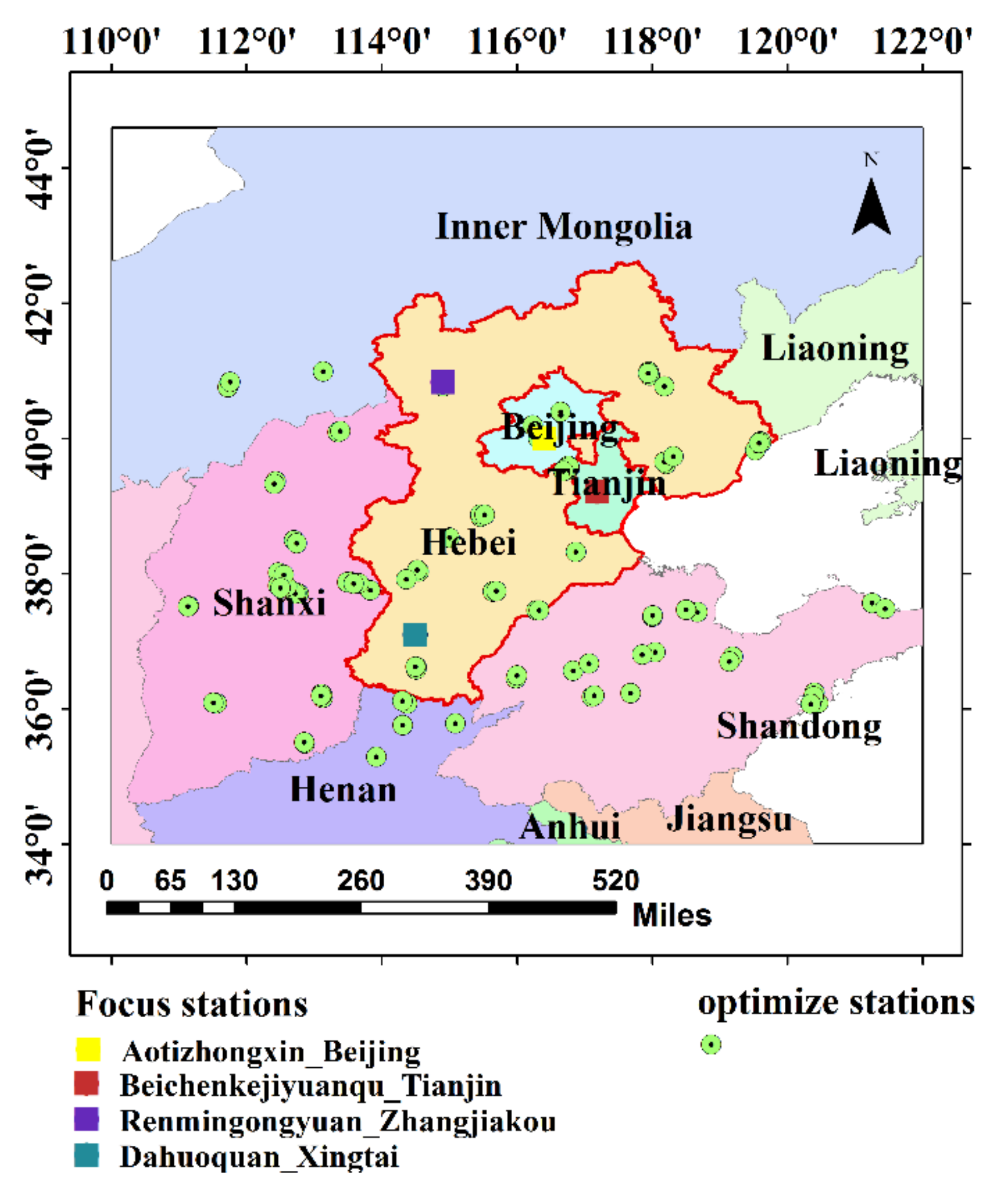
The Beijing-Tianjin-Hebei (BTH) region is located on the North China Plain. This region is the country’s main high-tech and heavy industry base, and it is also the location of China’s political and cultural center. These cities include Beijing, Tianjin, and 11 prefecture-level cities of the Hebei Province. The land area is 218,000 square kilometers, and the resident population is approximately 110 million people, of which 17.5 million are from outside areas. Economic development in the BTH region is accompanied by serious air pollution. Some studies have found that the BTH region is the most seriously polluted region in China [42,43,44,45]. According to China’s 2015 and 2016 Environmental Status Bulletin [46], PM2.5, as the main pollutant, has the largest number of days exceeding the standard in the BTH region, accounting for 68.4% and 63.1%, respectively [47]. Figure 1 is a sketch map of the study area in this research, and this area covers from 113.5° E to 119.8° E and from 36.0° N to 42.6° N.
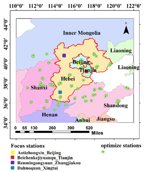
Figure 1.
The research area and observation sites. The optimized stations participate in optimizing the emission inventory of PM2.5 and the focus stations for result verification.
3. Materials and Methods
3.1. Model Development
The LPD model is developed based on the FLEXPART-WRF model, which employs the FLEXPART model to calculate the forward Lagrangian particle dispersion with driving data from the WRF model [48,49,50]. Compared with an adjoint Eulerian model, the advantage of the LPD model is that there is no initial diffusion due to the release of the adjoint tracer into a finite-size grid cell, which is independent from the computational grid. Furthermore, long-range transport can be simulated more accurately as no artificial numerical diffusion is present. The LPD model does not consider dry deposition or chemical reactions in the simulation of PM2.5, so it has low computational costs. The trajectories of individual particles are computed using a zero-acceleration scheme, in which particle movements are dependent on the grid scale winds and the turbulent fluctuations, which is shown as follows:
This equation is accurate to the first-order to integrate the trajectory equation [48]
where t is the time step, is the time increment, X is the position vector, and is the wind vector that is composed of the grid scale wind , the turbulent wind fluctuations , and the mesoscale wind fluctuations .
The LPD model makes it possible to obtain the contribution rate of each grid emission source to the receptors (observation sites), which provides the possibility to improve the prediction accuracy and analyze the contribution and spatial distribution of each type of pollution source (industry, power, residential, and transportation) to the site concentration of PM2.5. In addition, the forecast accuracy of the LPD model and the validity of the inventory inversion results have been verified and analyzed in previous studies, the prediction and inversion results are proved good [36,51]. In the following discussion, the receptors refer to the observation stations.
3.2. Methods
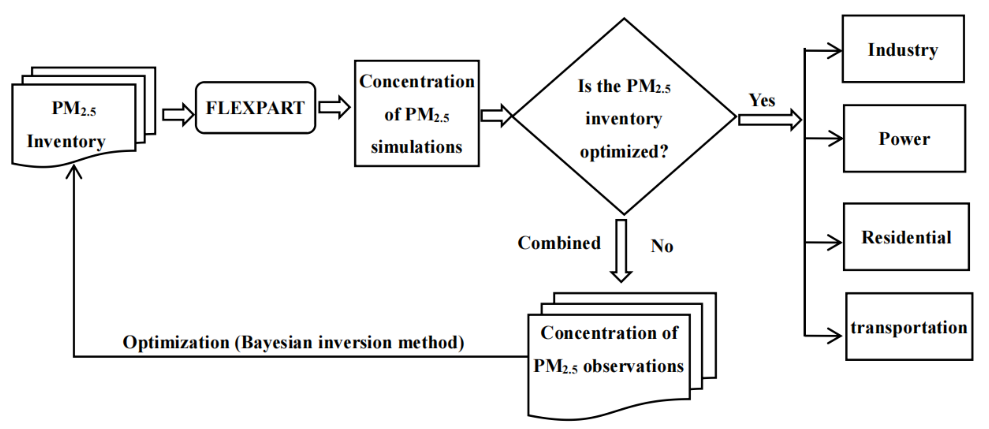
This section mainly includes two parts: inversion of the emission inventory of PM2.5 and the pollution source analysis of receptors of PM2.5, and the flowchart is shown in Figure 2. The a priori emission inventory and grid emission ratio (industry, power, transportation, and residential) of PM2.5 are from the Multiresolution emission inventory for China (MEIC) with a horizontal resolution of 0.25° 0.25° (http://www.meicmodel.org/ accessed on 22 March 2021). The PM2.5 observations were collected from the air quality observation datasets issued by the Ministry of Environmental Protection of China. The LPD drive data were provided by the Advanced Research WRF (WRW) version 4.0 modelling system.
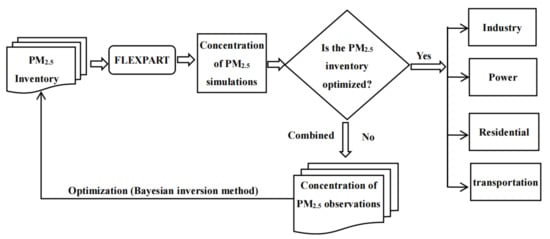
Figure 2.
Technical flow chart of the LPD model.
3.2.1. Inventory Inversion
In this research, the spatial distribution of the source-receptor relationship (SRR) was determined by the FLEXPART model. The SRR represents the contribution of each potential source to the receptors. In the present study, 30-day SRR was determined by releasing 10,000 particles from the potential sources per hour [51]. The Bayesian inversion method was used to combine the receptor observations to inverse the PM2.5 inventory. The principle of inversion is to optimize the emission flux density by minimizing the mismatch between the observed and simulated concentrations. The basic equation of the inversion approach can be written as follows:
where M is the matrix of SRR, is a vector of PM2.5 concentrations (μg/m3) at the receptor, and is the emission flux vector (Mg/grid/month). The equation can be written as follows:
where m is the time series of observations at the receptor and n is the number of emission grids. is a matrix that has m rows. Presuming that and where , and are referred to as a priori, a posteriori source vector, and observation vector, the cost function is described as follows:
The best estimate was obtained by solving equation as follows:
where and represent the standard errors related to the observations and a priori values, respectively. Considering that the inventory cannot be a negative, we need to have the condition . To reduce the unrealistic emissions in the posteriori region, the calculation was iterated until all negative emissions were greater than or equal to 0. Finally, the posteriori inventory was used to predict the PM2.5 concentration of receptors.
where t represents the time series of simulations in the future.
3.2.2. Source Analysis
The LPD model can simulate the contribution of each potential source of pollution to the receptor sites in real time. The PM2.5 emission inventory uses the 2016 MEIC products, which are divided into industrial, power, transportation, and residential emissions. The emission proportion of each source in each grid is calculated based on the MEIC PM2.5 emission inventory of 2016 (Figure 3), and the time resolution is monthly; that is, it is assumed that the emissions proportion of each source does not change within one month. The contribution of each pollution source (industry, electricity, transportation, and residential emission ratio) and the source spatial distribution of those pollutants to the receptors can be analyzed through the pollution emission source contribution of the receptors multiplied by the emission ratio of each grid point, which is described as follows:
where represents the forecasted concentration of PM2.5 at time t; represents the contribution of industrial sources to the forecasted concentration of the receptors at time t; represents the contribution of power sources to the forecasted concentration of the receptors at time t; represents the contribution of residential sources to the forecasted concentration of the receptors at time t; and represents the contribution of transportation sources to the forecasted concentration of the receptors at time t, where , , and can be obtained by Formula (11) as follow:
where represents the proportion of industrial emissions from the nth emission grid, represents the proportion of power emissions from the nth emission grid, represents the proportion of residential emissions from the nth emission grid, represents the proportion of transportation emissions from the nth emission grid, and represents the contribution of the nth emission grid to the concentration of receptors at time t, where , , and can be obtained by the MEIC PM2.5 emission inventory in 2016, and can be obtained from the LPD model.
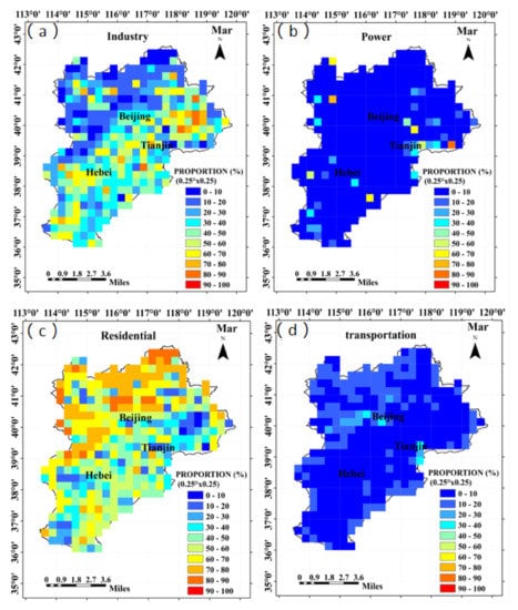
Figure 3.
Contribution rate of the PM2.5 emission source per grid (March 2016). In the figure, the letters represent industry emission sources (a); power emission sources (b); residential emission sources (c); and transportation emission sources (d).
3.3. Statistical Analysis Methods
To evaluate the accuracy of the concentration forecast and inventory inversion of the LPD model for PM2.5, the main statistical methods used in this article include the Pearson product-moment coefficient of linear correction, the root mean square error (RMSE) [52,53], and the index of agreement (IOA). The IOA index is defined as follows:
where is the th paired (model-observation) data point, is the total number of paired data points, and and are the th modelled and observed mixing ratios, respectively. Additionally, is the mean observed mixing ratio. The IOA value varies between 0.0 and 1.0, representing the limits of complete disagreement to perfect agreement, respectively, between the observations and simulations.
4. Results and Discussion
4.1. Evaluation of the Posteriori Inventory
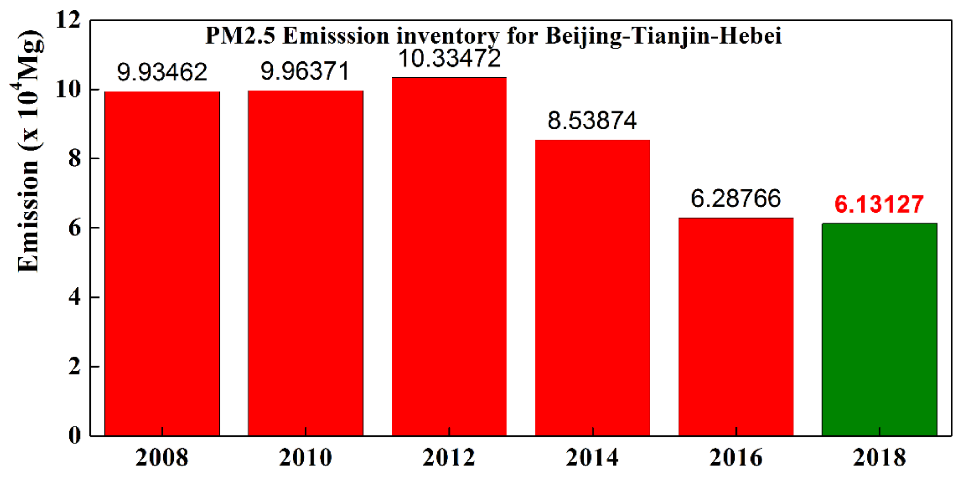
The inversion results of the PM2.5 inventory from the LPD model in January and February of 2018 will be used as the spin-up time and will not be part of the discussion of the results. The following series of discussions are based mainly on the results of the March 2018 period. Figure 4b shows the PM2.5 emission inventory in March 2018 retrieved by the LPD model for the BTH region, whose spatial distribution is basically consistent with the a priori inventory (Figure 4a), and the emissions have a certain degree of reduction compared with the a priori inventory. To show the spatial difference before and after the optimization inventory in the BTH region, the spatial difference between the posterior inventory and the a priori inventory is processed (Figure 4c), where blue and red represent the negative and positive differences between the two, respectively. The green column in Figure 5 is the posteriori inventory of PM2.5 statistics for the BTH region in March 2018, and the statistical results are basically consistent with the inventory of MEIC products (red column) in the corresponding months of 2016, which were 6.29 × 10⁴ Mg and 6.13 × 10⁴ Mg, respectively. In addition, Figure 5 shows that the annual emissions of PM2.5 pollution increased year by year from 2008 to 2012 and reached the maximum in 2012 [54]. In contrast, the annual emissions of PM2.5 decreased year by year from 2012 to 2018 and then reached a stable level in 2016. This result is mainly because the “Air Pollution Prevention and Control Action Plan” was issued by the State Council in 2013, and strict control measures have made the emissions of PM2.5 pollution decrease year by year since 2013 [55,56,57].
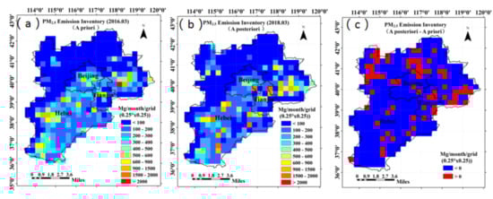
Figure 4.
PM2.5 emission inventory. In the figure, the letters represent a priori inventory (March 2016) (a); a posteriori inventory (2018.03) (b); the difference between a posteriori and a priori of inventory (c).
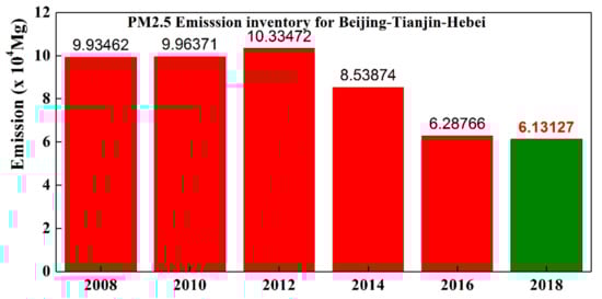
Figure 5.
PM2.5 Emission inventory for BTH (2018.03). The red and green histograms represent the MEIC datasets and the posteriori inventory statistical result of the BTH, respectively.
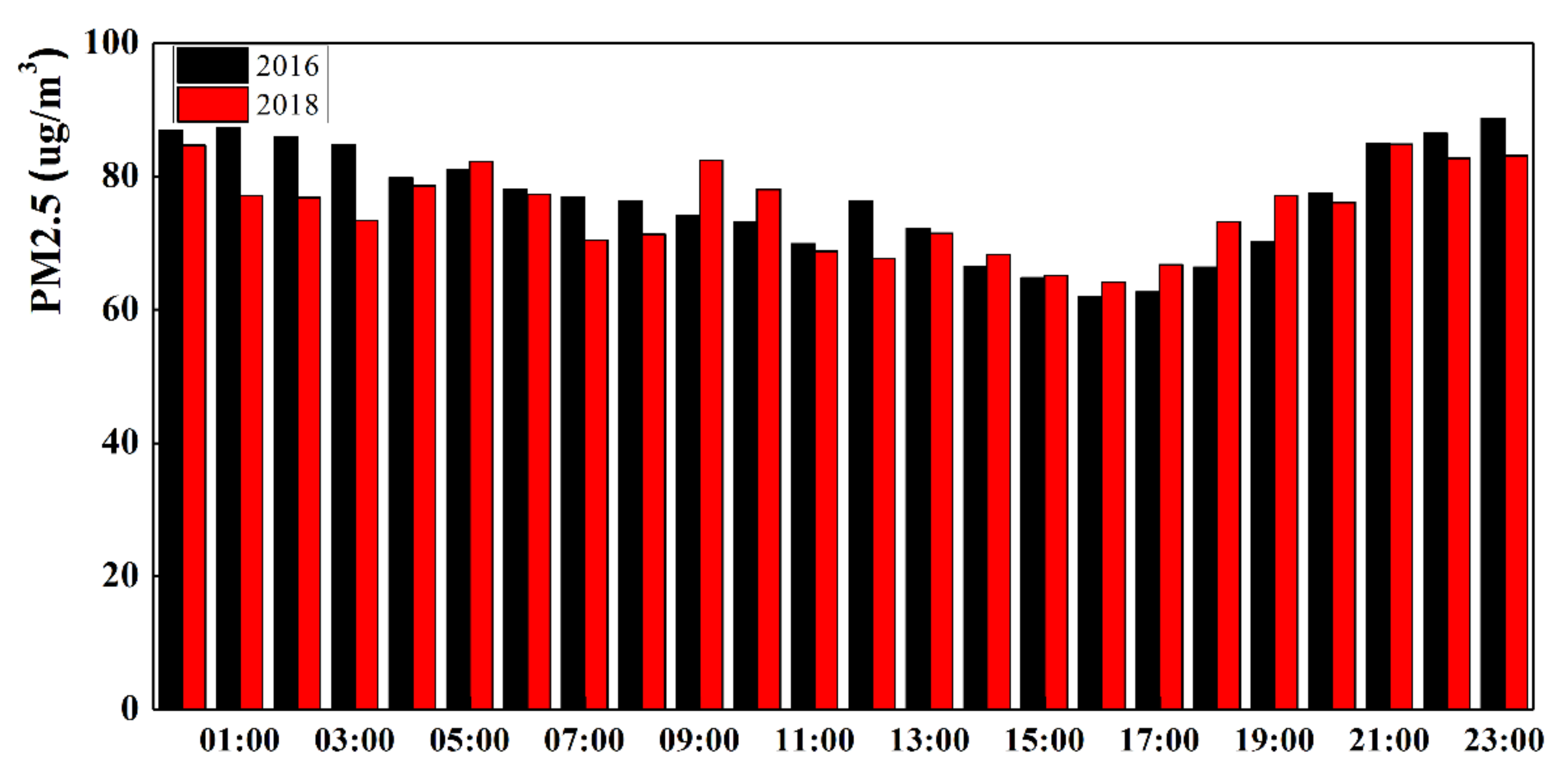
To verify the rationality of the posteriori inventory of PM2.5 inversion by the LPD model in March 2018, we analyzed the observations of the PM2.5 concentration in 2016 and 2018 (http://www.pm25.in/ accessed on 22 March 2021), and the results showed that the average hourly observations of the PM2.5 concentration in the BTH region in March 2018 changed in the same way as those in 2016 (Figure 6), which had values of 76.36 and 75.07 ug/m3 in March 2016 and March 2018, respectively. Ignoring the interannual differences in PM2.5 concentration caused by meteorological conditions, the variation trend and magnitude of the PM2.5 concentration were approximately the same as those in March 2016, which also verifies the rationality that the a posteriori inventory of PM2.5, that is, the a posteriori inventory of PM2.5 in 2018, is basically consistent with the MEIC inventory production in March 2016 (Figure 5). Notably, all the times used in this paper are Beijing Time (BJT).

Figure 6.
Hourly average of PM2.5 concentration in the BTH region. The black and red histograms represent the concentrations in 2016 and 2018, respectively.
4.2. Evaluation of Site Forecasts
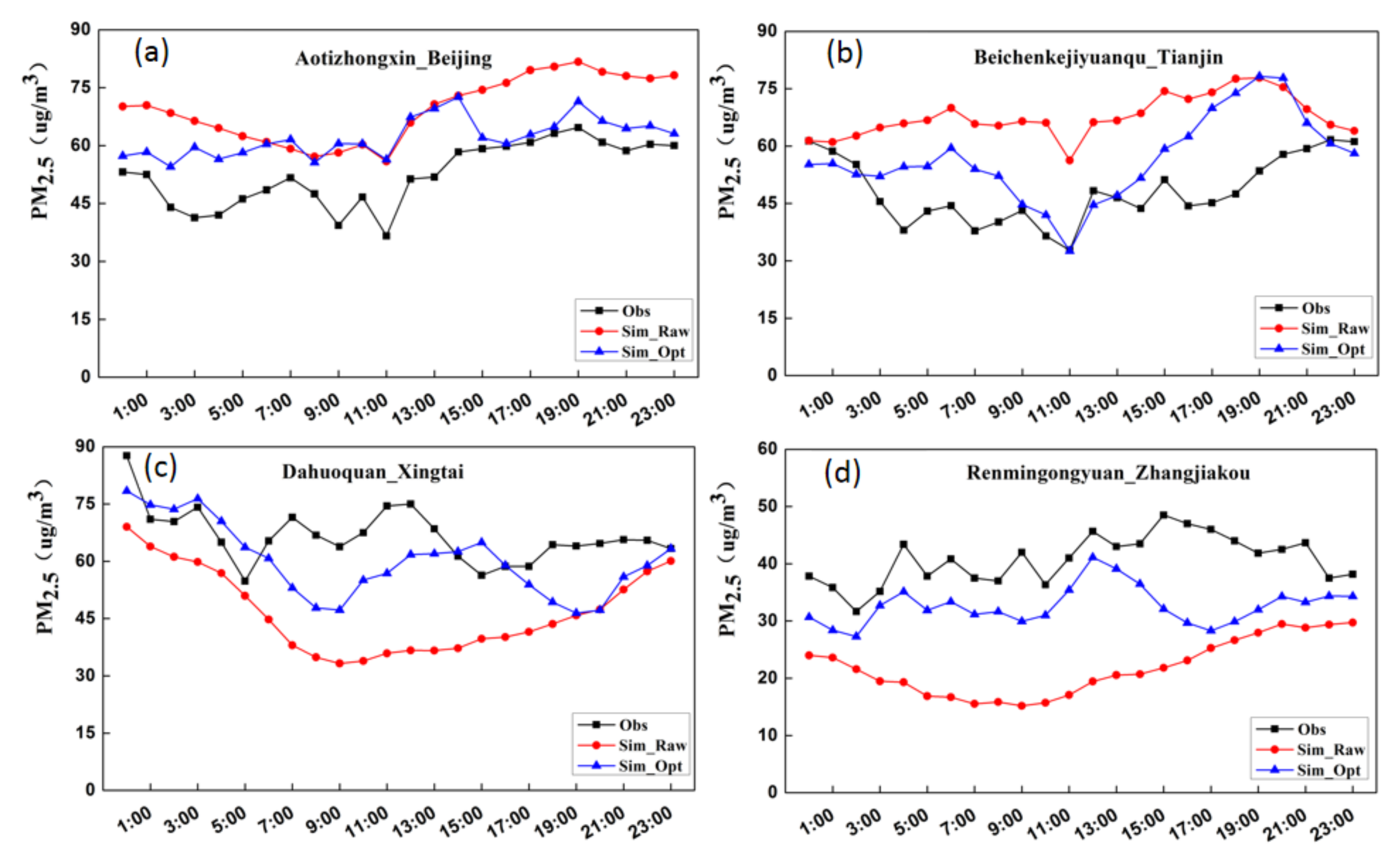
To evaluate the forecast effect of the LPD model after inventory optimization, the 6-day forecast results from 15–20 March 2018, were compared and analyzed with the observations (Figure 7) based on four observation sites in the BTH region (Aotizhongxin_Beijing, Beichenkejiyuanqu_Tianjin, Dahuoquan_Xintai, Renmingongyuan_Zhangjiakou). In Figure 7, Sim_Raw represents the hourly average concentration of PM2.5 that forecasts from the FLEXPART model based on the a priori inventory, Sim_Opt represents the hourly average concentration of PM2.5 that forecasts from the LPD based on the a posteriori inventory, and Obs represents the hourly average concentration of PM2.5 from the observation sites. The results show that the forecasted concentration of PM2.5 after inventory optimization is significantly better than that before inventory optimization. In Figure 7, the forecasted PM2.5 concentrations of the Aotizhongxin_Beijing and Beichenkejiyuanqu_Tianjin sites before inventory optimization are significantly higher than the observations. The Dahuoquan_Xingtai and Renmingongyuan_Zhangjiakou results are opposite, and their forecast concentrations of PM2.5 are significantly lower than the observations. The statistical results in Table 1 show that the correlation between the forecast concentration of PM2.5 of the LPD model after the inventory optimization and observations is increased by 9.66% compared to before optimization on average, the RMSE is reduced by 28.74%, and the IOA index is increased by 16.26%. In Table 1, the prefix RAW represents before the optimization of the inventory, and the prefix OPT represents after the optimization of the inventory, where INCREMENT = (OPT-RAW)/RAW. This result is mainly due to the Bayesian optimization method, which makes the PM2.5 emission inventory more reasonable and corrects part of the errors in the model simulation.
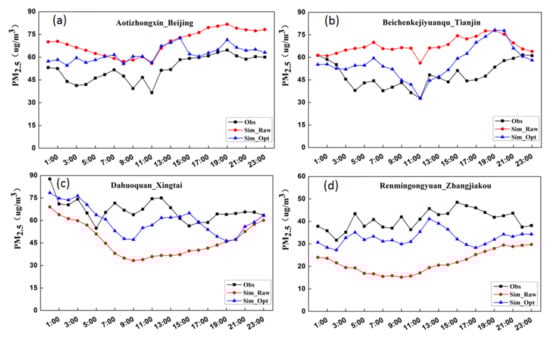
Figure 7.
Comparison of the hourly average of observations and forecasting values of PM2.5 concentrations. In the figure, the letters represent Aotizhongxin-Beijing (a); Beichenkejiyuanqu-Tianjin (b); Dahuoquan-Xingtai (c); and Renmingongyuan-Zhangjiakou (d).

Table 1.
Statistical analysis between the simulations of PM2.5 concentration based on the a priori inventory and the posteriori inventory and observations.
Additionally, we compared the prediction effect of the LPD model with the research results of other scholars. For example, Liu et al., (2020) evaluated the 5-day PM2.5 forecast results of three models on a daily scale: the CEEMD-GWO-SVR model proposed by Zhu et al., (2019), which combines the complementary ensemble empirical mode decomposition (CEEMD), grey wolf optimizer (GWO), and support vector regression (SVR) [58]; the wavelet-Ann model developed by Cheng et al., (2019) [59]; the WPD-PSO-BPNN-Adaboost model proposed by Liu et al., (2019), which contains the wavelet packet decomposition (WPD); and the prediction of a backpropagation neural network (BPNN) optimized by the particle swarm optimization (PSO) and adaptive boosting (Adaboost) algorithm [60]; the RMSEs of these three model forecast concentrations of PM2.5 in the BTH region are 37.4061 μg/m3, 34.8185 μg /m3, 27.8686 μg/m3, respectively [61]. These errors are higher than the results of concentrations of PM2.5 predicted by the LPD model using the posteriori inventory, in which RMSE with the observations is 23.41 μg/m3 on average. In addition, the LPD model can capture the concentration change information of PM2.5 at the hourly scale, which is more targeted for prevention and treatment. Guo et al., (2020) also compared the LPD forecasting model with the WRF-Chem and Camx models using data from monitoring stations in Xingtai, China, and the LPD forecasting model had higher accuracy than those models [51].
4.3. Analysis of the Spatiotemporal Forecasts of Pollution Sources
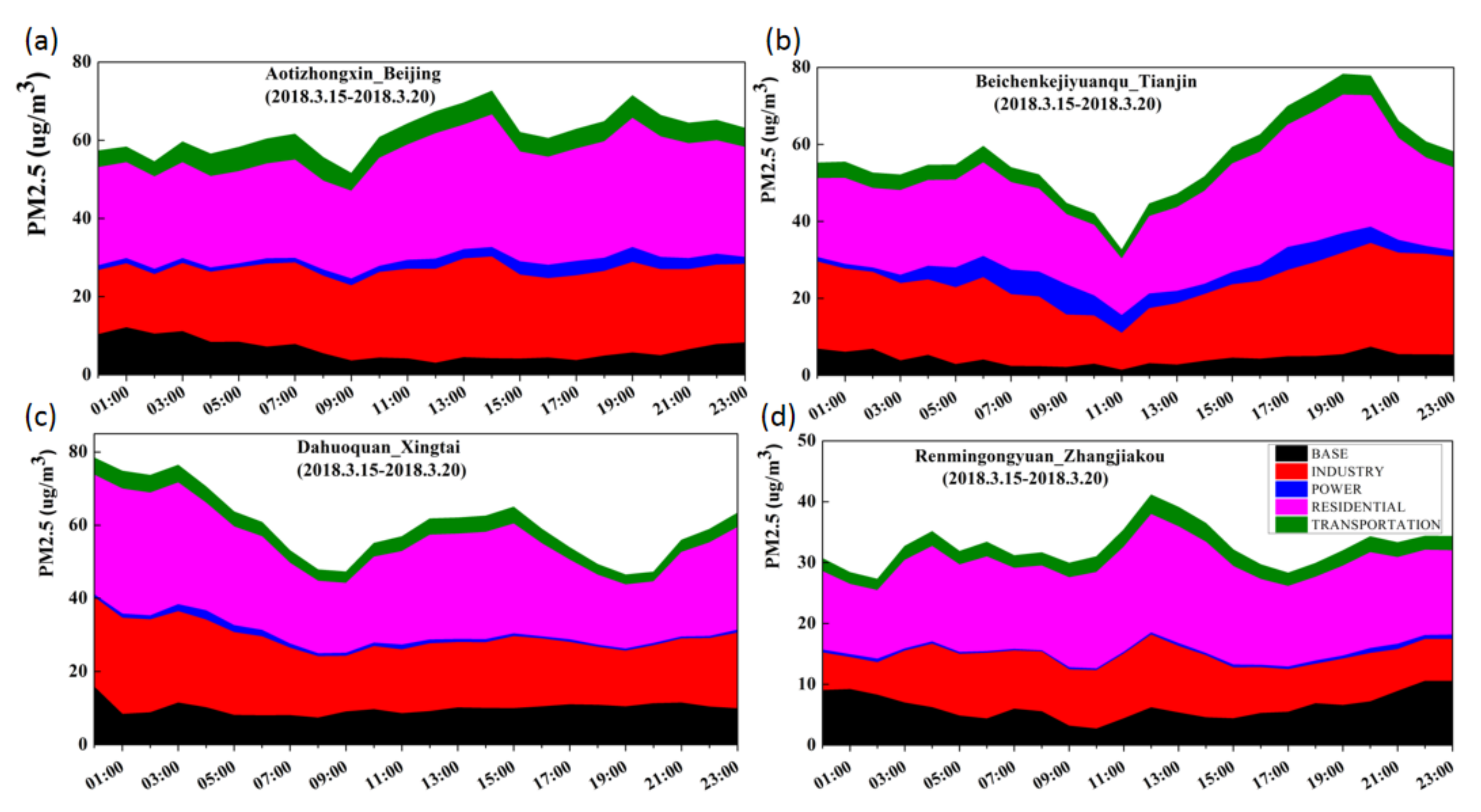
The LPD model improves the accuracies of the PM2.5 concentration forecasts at stations and predicts the pollution sources (industry, power, residence, and transportation) at the stations and their spatial distributions. Figure 8 shows the main pollution sources that caused the change in the PM2.5 concentrations at the stations from 15–20 March 2018. The black rendering represents the contribution of pollution sources outside the BTH region, and the red, blue, pink, and green renderings represent the contribution of industrial sources, power sources, residential sources, and transportation sources to the PM2.5 concentrations at the stations (Aotizhongxin_Beijing, Beichenkejiyuanqu_Tianjin, Dahuoquan_Xintai, Renmingongyuan_Zhangjiakou) in the BTH region, respectively. Figure 8 and the statistical analysis table (Table 2) show that the main pollution sources from 15–20 March 2018 originated from industrial and residential emissions, which are consistent with the previous sectoral analyzing results for other cities in BTH region [62]. In particular, residential emission sources contributed as much as 43.9% to the PM2.5 concentration at four stations in the BTH region, which was similar to a previous report that used the WRF-CMAQ model in December 2015, representing 46% of the monthly average concentration [63]. In addition, the results are consistent with the analytical results of modelling methods, and show that emissions from the residential contribute more to the PM2.5 concentration than the industrial sectors [64,65,66]. The result is reasonable and could be explained by an increase in residential coal usage due to heating during these colder seasons. In contrast, the power and transportation emission sources accounted for only a small proportion, especially the two monitoring stations in the Hebei Province (Dahuoquan_Xintai and Renmingongyuan_Zhangjiakou stations), which had little influence from power sources, and the rates were 1.72% and 1.39%, respectively. The contribution rates of the surrounding pollution sources to the two monitoring stations (Dahuoquan_Xintai and Renmingongyuan_Zhangjiakou) in the Hebei Province for the PM2.5 concentration were 16.44% and 19.39%, respectively, which were 8.9% higher than the Aotizhongxin_Beijing and Beichenkejiyuanqu_Tianjin sites, and the rates were 10.36% and 7.62%, respectively. A similar phenomenon was previously reported; for example, Zhang et al., (2017) used the WRF-Chem model to analyze the impact of the surrounding pollution sources on the BTH region, and the results showed that the surrounding pollution sources contributing to the PM2.5 concentration in the BTH region were approximately 9.3% [67]. Although different models, simulation times, and input data have a great influence on the analytical results, the research results of previous studies and this paper show that the PM2.5 concentration contribution in the BTH region mainly originates from local pollution sources, and this information can be targeted to control and prevent the occurrence of pollution events.
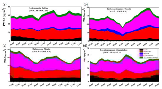
Figure 8.
Pollution source forecast of PM2.5 concentrations at sites. In the figure, the letters represent Aotizhongxin-Beijing (a), Beichenkejiyuanqu-Tianjin (b), Dahuoquan-Xingtai (c), and Renmingongyuan-Zhangjiakou (d).
Table 2.
Contribution rate of each pollution source to the PM2.5 concentration at each site.
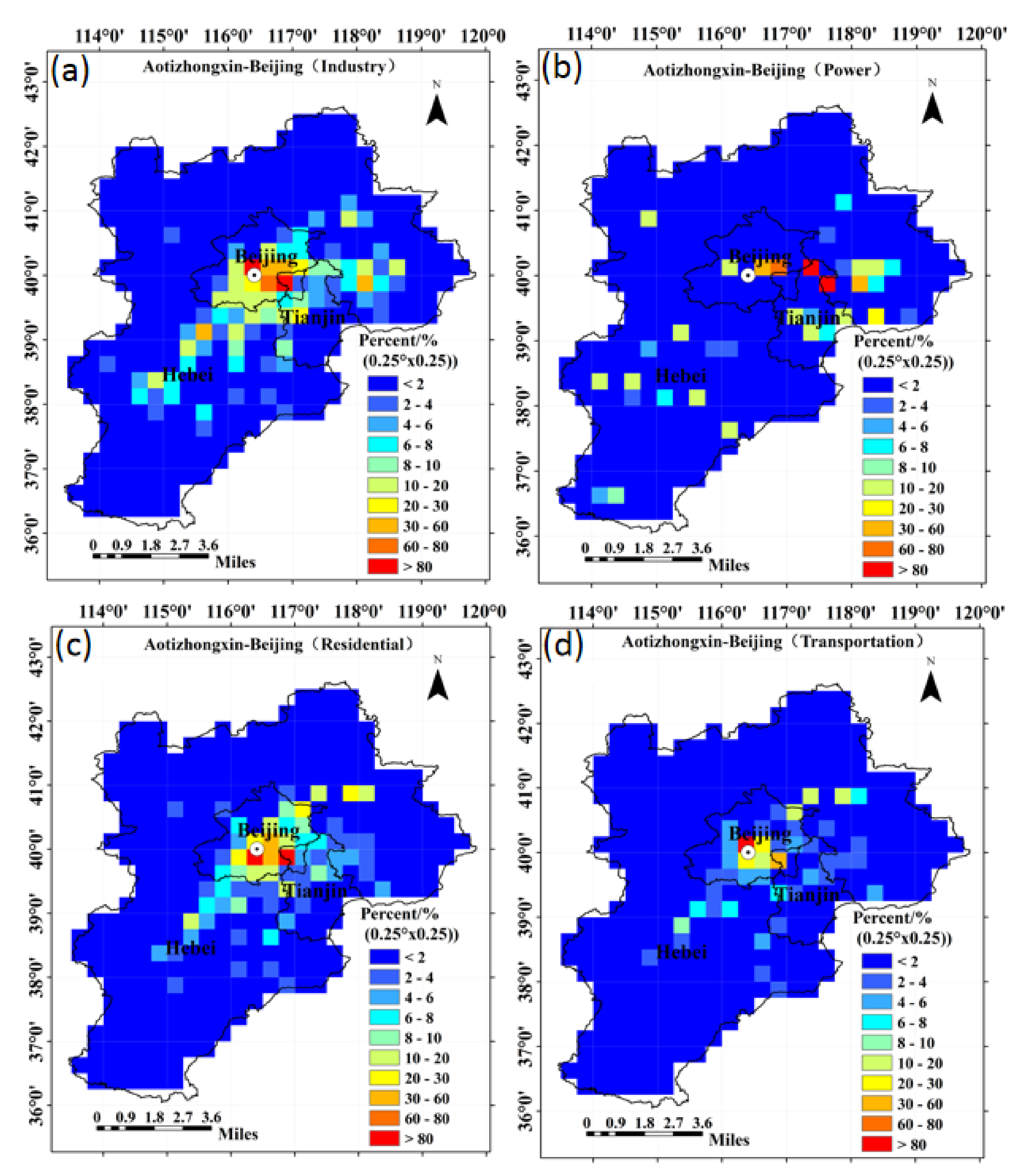
Figure 9 shows the spatial distribution of each type of pollution source that led to the PM2.5 concentration change at the Aotizhongxin_Beijing station from 15–20 March 2018, simulated by the LPD model. This distribution map is the ratio between the grid contribution of the corresponding pollution source to the Aotizhongxin_Beijing station and the maximum grid contribution to the Aotizhongxin_Beijing station of this type of pollution source in the BTH region, with a spatial resolution of 0.25° × 0.25°. Red represents the grid values where the corresponding pollution sources (industry, power, residence, and transportation) contribute more to the site concentration of PM2.5, and blue represents the corresponding types of pollution sources that contribute less to the site concentration of PM2.5. During this forecast period (15–20 March 2018), the surrounding industrial and residential emission sources have a greater influence on the Aotizhongxin_Beijing station over a wide range. In contrast, the power and transportation sources have a small influence on the Aotizhongxin_Beijing station. In particular, the influence of the power source on the Aotizhongxin_Beijing station is relatively scattered (Figure 9b).

Figure 9.
The spatial distribution map of the contribution rate of each pollution source to the PM2.5 concentration at Aotizhongxin_Beijing (15–20 March 2018). In the figure, the letters represent industry (a), power (b), residential (c), and transportation (d).
5. Conclusions
LPD can improve PM2.5 concentration forecast accuracy by optimizing the PM2.5 emission inventory and by obtaining real-time analyses of the temporal and spatial distributions and pollution source contributions that lead to changes in the PM2.5 concentration at the receptors. This model was applied to the BTH region, which has severe pollution, and the hourly forecast values over 6 days from 15–20 March 2018 were analyzed. The results show that the average correlation between the forecasted concentrations of PM2.5 after the emission inventory was optimized and that the observations were as high as ~0.82 at four observation sites (Aotizhongxin_Beijing, Beichenkejiyuanqu_Tianjin, Dahuoquan_Xintai, Renmingongyuan_Zhangjiakou); the RMSE was ~23.41, and the IOA index was ~0.84, which was significantly improved compared to the values obtained before inventory optimization.
During this period (15–20 March 2018), the main pollution sources that led to the changes in the concentrations of PM2.5 at the four observation sites originated from industrial and residential emissions, and power and transportation pollution sources accounted for only a small proportion, especially the Dahuoquan_Xintai and Renmingongyuan_Zhangjiakou stations in the Hebei Province; power pollution sources had little influence on these stations, and the values were 1.72% and 1.39%, respectively. The influence of the surrounding pollution sources from outside BTH on the Dahuoquan_Xintai and Renmingongyuan_Zhangjiakou stations in the Hebei Province was 16.44% and 19.39%, respectively. Compared with the Aotizhongxin_Beijing and Beichenkejiyuanqu_Tianjin sites, the average influence ratio increased by 8.9%.
Considering the actual situation and operating efficiency of the LPD model, the concentration forecast of PM2.5 and the analysis of each type of pollution source are only at the site scale, without considering dry and wet sedimentation and chemical reactions of the particles, and this part of the error is attributed to the uncertainties in both the model and emission inventory. The reader should keep in mind that inverse approaches still have large uncertainties due to the limited observation sites and the method bias. Therefore, the LPD model needs to be further optimized and expanded in future research for the development of forecasting surface-level distributions of PM2.5 concentration and each type of pollution source analysis at a regional scale. In addition, at present, we only quantitatively evaluate the reliability of the LPD model and input the parameters through indirect or by comparison with observations, and we need to further verify and analyze its reliability and adaptability.
Author Contributions
Conceptualization, B.C.; Methodology, B.C. and L.G.; Software, L.G.; Validation, L.G. and J.F.; Formal Analysis, L.G.; Investigation, L.G.; Resources, B.C.; Data Curation, L.G., H.Z. and J.F.; Writing–Original Draft Preparation, L.G. and B.C.; Writing–Review & Editing, B.C.; Visualization, L.G., H.Z. and J.F. Supervision, B.C.; Project Administration, B.C.; Funding Acquisition, B.C. All authors have read and agreed to the published version of the manuscript.
Funding
This work was supported by National Key R&D Program of China [Grant # 2018YFA0606001 & 2017YFA0604302], the research grants [41771114 & 41977404] funded by the National Natural Science Foundation of China, and the research grant [O88RA901YA] funded by the State Key Laboratory of Resources and Environment Information System.
Data Availability Statement
The data presented in this study are available on request from the corresponding author.
Acknowledgments
We thank Qiang Zhang’s team from the Tsinghua University for providing the multiscale emission inventory of China’s (MEIC) data.
Conflicts of Interest
The authors declare no conflict of interest.
References
- Zhao, X.; Shi, H.; Yu, H.; Yang, P. Inversion of Nighttime PM2.5 Mass Concentration in Beijing Based on the VIIRS Day-Night Band. Atmosphere 2016, 7, 136. [Google Scholar] [CrossRef] [Green Version]
- Huang, R.-J.; Zhang, Y.; Bozzetti, C.; Ho, K.-F.; Cao, J.-J.; Han, Y.; Daellenbach, K.R.; Slowik, J.G.; Platt, S.M.; Canonaco, F.; et al. High secondary aerosol contribution to particulate pollution during haze events in China. Nature 2014, 514, 218. [Google Scholar] [CrossRef] [PubMed] [Green Version]
- Qiu, J.; Wang, H.; Zhou, X.; Lu, D. Experimental Study Of Remote Sensing Of Atmospheric Aerosol Size Distribution By Combined Solar Extinction And Forward Scattering Method. Adv. Atmos. Sci. 1985, 2, 307–315. [Google Scholar] [CrossRef]
- Watson, J.G. Visibility: Science and Regulation. J. Air Waste Manag. Assoc. 2002, 52, 628–713. [Google Scholar] [CrossRef] [Green Version]
- Hyslop, N.P. Impaired visibility: The air pollution people see. Atmos. Environ. 2009, 43, 182–195. [Google Scholar] [CrossRef]
- Gao, B.; Hai, G.; Wang, X.M.; Zhao, X.Y.; Ling, Z.H.; Zhou, Z.; Liu, T.Y. Polycyclic aromatic hydrocarbons in PM2.5 in Guangzhou, southern China: Spatiotemporal patterns and emission sources. J. Hazard. Mater. 2012, 239–240, 78–87. [Google Scholar] [CrossRef]
- Wang, N.; Ling, Z.; Deng, X.; Deng, T.; Lyu, X.; Tingyuan, L.I.; Gao, X.; Chen, X. Source Contributions to PM2.5 under Unfavorable Weather Conditions in Guangzhou City, China. Adv. Atmos. Sci. 2018, 35, 1145–1159. [Google Scholar] [CrossRef]
- Pope, C.A.; Ezzati, M.; Dockery, D.W. Fine-particulate air pollution and life expectancy in the United States. N. Engl. J. Med. 2009, 360, 376. [Google Scholar] [CrossRef] [Green Version]
- Tie, X.; Wu, D.; Brasseur, G. Lung cancer mortality and exposure to atmospheric aerosol particles in Guangzhou, China. Atmos. Environ. 2009, 43, 2375–2377. [Google Scholar] [CrossRef]
- IPCC. Climate Change 2013: The Physical Science Basis; Contribution of Working Group I Contribution to the Fifth Assessment Report of the International Panel on Climate Change; Cambridge University Press: Cambridge, MA, USA, 2013. [Google Scholar]
- Yan, D.Y.; Kong, Y.B.; Xiang, H. Spatio-temporal variation and daily prediction of PM2.5 concentration in world-class urban agglomerations of China. Environ. Geochem. Health 2021, 43, 301–316. [Google Scholar] [CrossRef]
- Feng, J.; Yu, H.; Liu, S.; Su, X.; Li, Y.; Pan, Y.; Sun, J. PM2.5 levels, chemical composition and health risk assessment in Xinxiang, a seriously air-polluted city in North China. Environ. Geochem. Health 2016, 39, 1071–1083. [Google Scholar] [CrossRef]
- Shang, Z.; Deng, T.; He, J.; Duan, X. A novel model for hourly PM2.5 concentration prediction based on CART and EELM. Sci. Total Environ. 2018, 651, 3043–3052. [Google Scholar] [CrossRef]
- Qin, S.; Liu, F.; Wang, J.; Sun, B. Analysis and forecasting of the particulate matter (PM) concentration levels over four major cities of China using hybrid models. Atmos. Environ. 2014, 98, 665–675. [Google Scholar] [CrossRef]
- Huang, G.; Li, X.; Zhang, B.; Ren, J. PM2.5 Concentration Forecasting at Surface Monitoring Sites Using GRU Neural Network Based on Empirical Mode Decomposition. Sci. Total Environ. 2021, 768, 144516. [Google Scholar] [CrossRef]
- Wen, C.; Liu, S.; Yao, X.; Peng, L.; Li, X.; Hu, Y.; Chi, T. A novel spatiotemporal convolutional long short-term neural network for air pollution prediction. Sci. Total Environ. 2019, 654, 1091–1099. [Google Scholar] [CrossRef]
- Zhu, J.; Deng, F.; Zhao, J.; Zheng, H. Attention-based parallel networks (APNet) for PM2.5 spatiotemporal prediction—ScienceDirect. Sci. Total Environ. 2021, 769, 145082. [Google Scholar] [CrossRef]
- Gupta, P.; Christopher, S.A. Particulate matter air quality assessment using integrated surface, satellite, and meteorological products: Multiple regression approach. J. Geophys. Res. Atmos. 2009, 114, D14. [Google Scholar] [CrossRef] [Green Version]
- Vlachogianni, A.; Kassomenos, P.; Karppinen, A.; Karakitsios, S.; Kukkonen, J. Evaluation of a multiple regression model for the forecasting of the concentrations of NOx and PM10 in Athens and Helsinki. Sci. Total Environ. 2011, 409, 1559–1571. [Google Scholar] [CrossRef]
- Garcia, J.M.; Teodoro, F.; Cerdeira, R.; Coelho, L.M.R.; Prashant, K.; Carvalho, M.G. Developing a methodology to predict PM10 concentrations in urban areas using generalized linear models. Environ. Technol. 2016, 37, 2316–2325. [Google Scholar] [CrossRef] [Green Version]
- Loy-Benitez, J.; Vilela, P.; Li, Q.; Yoo, C. Sequential prediction of quantitative health risk assessment for the fine particulate matter in an underground facility using deep recurrent neural networks. Ecotoxicol. Environ. Saf. 2019, 169, 316–324. [Google Scholar] [CrossRef]
- Tong, W.; Li, L.; Zhou, X.; Hamilton, A.; Zhang, K. Deep learning PM2.5 concentrations with bidirectional LSTM RNN. Air Qual. Atmos. Health 2019, 12, 411–423. [Google Scholar] [CrossRef]
- Tharwat, E. Alhanafy, Fareed Zaghlooland Abdou Saad El Din Moustafa. Neuro Fuzzy Modeling Scheme for the Prediction of Air Pollution. J. Am. Sci. 2010, 6, 605–616. [Google Scholar]
- Goyal, P.; Chan, A.T.; Jaiswal, N. Statistical models for the prediction of respirable suspended particulate matter in urban cities. Atmos. Environ. 2006, 40, 2068–2077. [Google Scholar] [CrossRef]
- Islam, M.M.; Sharmin, M.; Ahmed, F. Predicting air quality of Dhaka and Sylhet divisions in Bangladesh: A time series modeling approach. Air Qual. Atmos. Health 2020, 13, 607–615. [Google Scholar] [CrossRef]
- Biancofiore, F.; Busilacchio, M.; Verdecchia, M.; Tomassetti, B.; Aruffo, E.; Bianco, S.; Tommaso, S.D.; Colangeli, C.; Rosatelli, G.; Carlo, P.D. Recursive neural network model for analysis and forecast of PM10 and PM2.5. Atmos. Pollut. Res. 2017, 8, 652–659. [Google Scholar] [CrossRef]
- Rahimi, A. Short-term prediction of NO2 and NOx concentrations using multilayer perceptron neural network: A case study of Tabriz, Iran. Ecol. Process. 2017, 6, 1–9. [Google Scholar] [CrossRef] [Green Version]
- Xiao, F.; Qi, L.; Zhu, Y.; Hou, J.; Jin, L.; Wang, J. Artificial neural networks forecasting of PM2.5 pollution using air mass trajectory based geographic model and wavelet transformation. Atmos. Environ. 2015, 107, 118–128. [Google Scholar]
- Mao, X.; Shen, T.; Feng, X. Prediction of hourly ground-level PM2.5 concentrations 3 days in advance using neural networks with satellite data in eastern China. Atmos. Pollut. Res. 2017, 8, 1005–1015. [Google Scholar] [CrossRef]
- Qi, Y.; Li, Q.; Karimian, H.; Liu, D. A hybrid model for spatiotemporal forecasting of PM2.5 based on graph convolutional neural network and long short-term memory. Ence Total Environ. 2019, 664, 1–10. [Google Scholar] [CrossRef]
- Heald, C.L.; Henze, D.K.; Horowitz, L.W.; Feddema, J.; Lamarque, J.F.; Guenther, A.; Hess, P.G.; Vitt, F.; Seinfeld, J.H.; Goldstein, A.H. Predicted change in global secondary organic aerosol concentrations in response to future climate, emissions, and land use change. J. Geophys. Res. Atmos. 2008, 113, 79–88. [Google Scholar] [CrossRef]
- Kukkonen, J.; Partanen, L.; Karppinen, A.; Ruuskanen, J.; Junninen, H.; Kolehmainen, M.; Niska, H.; Dorling, S.; Chatterton, T.; Foxall, R.; et al. Extensive evaluation of neural network models for the prediction of NO2 and PM10 concentrations, compared with a deterministic modelling system and measurements in central Helsinki. Atmos. Environ. 2003, 37, 4539–4550. [Google Scholar] [CrossRef]
- Qie, G.; Wang, Y.; Wu, C.; Mao, H.; Zhang, P.; Li, T.; Li, Y.; Talbot, R.; Hou, C.; Yue, T. Distribution and sources of particulate mercury and other trace elements in PM2.5 and PM10 atop Mount Tai, China. J. Environ. Manag. 2018, 215, 195–205. [Google Scholar] [CrossRef] [Green Version]
- Draxler, R.R.; Hess, G.D. Description of the Hysplit_4 Modeling System; NOAA Tech Memo, ERL ARL-224, NOAA; Air Resources Laboratory: Silver Spring, MD, USA, 1997; Volume 24. [Google Scholar]
- Caili, L.; Shaoqing, Z.; Yang, G.; Yuhang, W.; Lifang, S.; Huiwang, G.; Fung, J.C.H. Optimal estimation of initial concentrations and emission sources with 4D-Var for air pollution prediction in a 2D transport model. Sci. Total Environ. 2021, 773, 145580. [Google Scholar]
- Guo, L.; Chen, B.; Zhang, H.; Xu, G.; Lu, L.; Lin, X.; Kong, Y.; Wang, F.; Li, Y. Improving PM2.5 Forecasting and Emission Estimation Based on the Bayesian Optimization Method and the Coupled Flexpart-Wrf Model. Atmosphere 2018, 9, 428. [Google Scholar] [CrossRef] [Green Version]
- Oliver, J.G.J.; Bouwman, A.F.; van der Maas, C.W.N.; Berdowski, J.J.M.; Veldt, C.; Bloos, J.P.J.; Visschedijk, A.J.H.; Zandveld, P.Y.J.; Haverlag, J.L. Description of EDGAR Version 2.0: A Set of Global Emission Inventories of Greenhouse Gases and Ozonedepleting Substances for All Anthropogenic and Most Natural Sources on a Per Country Basis and on 1 Degree x 1 Degree Grid. RIVM/TNO Rep. 771060-002; Rijksinstituut voor Volksgezondheid en Milieu: Bilthoven, The Netherlands, 1996; 140p. [Google Scholar]
- Zhang, Q.; Streets, D.G.; Carmichael, G.R.; He, K.B.; Huo, H.; Kannari, A.; Klimont, Z.; Park, I.S.; Reddy, S.; Fu, J.S.; et al. Asian emissions in 2006 for the NASA INTEX-B mission. Atmos. Chem. Phys. 2009, 9, 5131–e5153. [Google Scholar] [CrossRef] [Green Version]
- Zhao, Y.; Feng, L.; Wang, Y.; Shang, B.; Han, P. Study on Pollution Characterization and Source Apportionment of Daytime and Nighttime PM2.5 Samples in an Urban Residential Community in Different Weather Conditions. Bull. Environ. Contam. Toxicol. 2020, 104, 673–681. [Google Scholar] [CrossRef]
- Fan, X.; Chen, Z.; Liang, L.; Qiu, G. Atmospheric PM2.5—Bound Polycyclic Aromatic Hydrocarbons (PAHs) in Guiyang City, Southwest China: Concentration, Seasonal Variation, Sources and Health Risk Assessment. Arch. Environ. Contam. Toxicol. 2018, 76, 102–113. [Google Scholar] [CrossRef]
- Hu, R.; Liu, G.; Hong, Z.; Xue, H.; Xin, W. Levels and Sources of PAHs in Air-borne PM2.5 of Hefei City, China. Bull. Environ. Contam. Toxicol. 2017, 98, 270–276. [Google Scholar] [CrossRef]
- Yu, H.; Feng, J.; Su, X.; Li, Y.; Sun, J. A seriously air pollution area affected by anthropogenic in the central China: Temporal-spatial distribution and potential sources. Environ. Geochem. Health 2020, 42, 3199–3211. [Google Scholar] [CrossRef]
- Wu, D.; Wu, X.J.; Li, F. Temporal and spatial variation of haze during 1951–2005 in Chinese mainland. J. Meteorol. Res. 2010, 68, 680–688. [Google Scholar]
- Hu, J.; Wang, Y.; Qi, Y.; Zhang, H. Spatial and temporal variability of PM2.5 and PM10 over the North China Plain and the Yangtze River Delta, China. Atmos. Environ. 2014, 95, 598–609. [Google Scholar] [CrossRef]
- Tan, J.; Duan, J.; Zhen, N.; He, K.; Hao, J. Chemical characteristics and source of size-fractionated atmospheric particle in haze episode in Beijing. Atmos. Res. 2015, 167, 24–33. [Google Scholar] [CrossRef]
- Ministry of Environmental Protection P.R.C. (MEP). China Environmental Status Bulletin; MEP: Beijing, China, 2017. (In Chinese)
- Zhang, Q.; Tong, P.; Liu, M.; Lin, H.; Wang, X. A WRF-Chem model-based future vehicle emission control policy simulation and assessment for the Beijing-Tianjin-Hebei region, China. J. Environ. Manag. 2019, 253, 109751. [Google Scholar] [CrossRef]
- Stohl, A.; Hittenberger, M.; Wotawa, G. Validation of the Lagrangian particle dispersion model FLEXPART against large-scale tracer experiment data. Atmos. Environ. 1998, 32, 4245–4264. [Google Scholar] [CrossRef]
- Fast, J.D.; Easter, R.C. A Lagrangian particle dispersion model compatible with WRF. In Proceedings of the 7th Annual WRF User’s Workshop, Boulder, CO, USA, 19–22 June 2006. [Google Scholar]
- Bei, N.; Bo, X.; Ning, M.; Tian, F. Critical role of meteorological conditions in a persistent haze episode in the Guanzhong basin, China. Sci. Total Environ. 2016, 550, 273–284. [Google Scholar] [CrossRef]
- Guo, L.; Chen, B.; Zhang, H.; Zhang, Y. A new approach combining a simplified FLEXPART model and a Bayesian-RAT method for forecasting PM10 and PM2.5. Environ. Sci. Pollut. Res. 2020, 27, 2165–2183. [Google Scholar] [CrossRef]
- Willmott, C.J.; Matsuura, K. Advantages of the mean absolute error (MAE) over the root mean square error (RMSE) in assessing average model performance. Clim. Res. 2005, 30, 79. [Google Scholar] [CrossRef]
- Willmott, C.J.; Ackleson, S.G.; Davis, R.E.; Feddema, J.J.; Klink, K.M.; Legates, D.R.; O’Donnell, J.; Rowe, C.M. Statistics for the evaluation and comparison of models. J. Geophys. Res. Oceans. 1985, 90, 8995–9005. [Google Scholar] [CrossRef] [Green Version]
- Li, M.; Zhang, Q.; Kurokawa, J.-I.; Woo, J.-H.; He, K.; Lu, Z.; Ohara, T.; Song, Y.; Streets, D.G.; Carmichael, G.R.; et al. MIX: A mosaic Asian anthropogenic emission inventory under the international collaboration framework of the MICS-Asia and HTAP. Atmos. Chem. Phys. 2017, 17, 935–963. [Google Scholar] [CrossRef] [Green Version]
- Qi, M.; Wang, L.; Ma, S.; Zhao, L.; Xu, R. Evaluation of PM2.5 fluxes in the “2+26” cities: Transport pathways and intercity contributions. Atmos. Pollut. Res. 2021, 12, 101048. [Google Scholar] [CrossRef]
- Chen, Z.; Chen, D.; Wen, W.; Zhuang, Y.; Kwan, M.P.; Chen, B.; Zhao, B.; Yang, L.; Gao, B.; Li, R. Evaluating the “2+ 26” regional strategy for air quality improvement during two air pollution alerts in Beijing: Variations in PM 2.5 concentrations, source apportionment, and the relative contribution of local emission and regional transport. Atmos. Chem. Phys. 2019, 19, 6879–6891. [Google Scholar] [CrossRef] [Green Version]
- Zhu, Y.Y.; Gao, Y.X.; Wang, W.; Lu, N.; Li, J.J. Assessment of Emergency Emission Reduction Effect During the Heavy Air Pollution Episodes in Beijing, Tianjin, Hebei, and Its Surrounding Area (“2+26” Cities) from October to December 2019. Huan Jing Ke Xue Huanjing Kexue 2020, 41, 4402–4412. [Google Scholar] [PubMed]
- Zhu, S.; Qiu, X.; Yin, Y.; Fang, M.; Liu, X.; Zhao, X.; Shi, Y. Two-step-hybrid model based on data preprocessing and intelligent optimization algorithms (CS and GWO) for NO2 and SO2 forecasting. Atmos. Pollut. Res. 2019, 10, 1326–1335. [Google Scholar] [CrossRef]
- Cheng, Y.; Zhang, H.; Liu, Z.; Chen, L.; Wang, P. Hybrid algorithm for short-term forecasting of PM2.5 in China. Atmos. Environ. 2019, 200, 264–279. [Google Scholar] [CrossRef]
- Liu, H.; Jin, K.; Duan, Z. Air PM2.5 concentration multi-step forecasting using a new hybrid modeling method: Comparing cases for four cities in China. Atmos. Pollut. Res. 2019, 10, 1588–1600. [Google Scholar] [CrossRef]
- Liu, H.; Chen, C. Prediction of outdoor PM2.5 concentrations based on a three-stage hybrid neural network model. Atmos. Pollut. Res. 2020, 11, 469–481. [Google Scholar] [CrossRef]
- Wang, L.; Wei, Z.; Wei, W.; Fu, J.S.; Meng, C.; Ma, S. Source apportionment of PM2.5 in top polluted cities in Hebei, China using the CMAQ model. Atmos. Environ. 2015, 122, 723–736. [Google Scholar] [CrossRef]
- Zhang, Z.; Wang, W.; Cheng, M.; Liu, S.; Xu, J.; He, Y.; Meng, F. The contribution of residential coal combustion to PM2.5 pollution over China’s Beijing-Tianjin-Hebei region in winter. Atmos. Environ. 2017, 159, 147–161. [Google Scholar] [CrossRef]
- Tian, Y.Z.; Chen, G.; Wang, H.T.; Huang-Fu, Y.Q.; Shi, G.L.; Han, B.; Feng, Y.C. Source regional contributions to PM2.5 in a megacity in China using an advanced source regional apportionment method. Chemosphere 2016, 147, 256–263. [Google Scholar] [CrossRef]
- Zhe, W.; Wang, L.; Chen, M.; Yan, Z. The 2013 severe haze over the Southern Hebei, China: PM2.5 composition and source apportionment. Atmos. Pollut. Res. 2014, 5, 759–768. [Google Scholar]
- Jin, X.; Xiao, C.; Li, J.; Huang, D.; Ni, B. Source apportionment of PM2.5 in Beijing using positive matrix factorization. J. Radioanal. Nucl. Chem. 2015, 307, 2147–2154. [Google Scholar] [CrossRef]
- Zhang, Y.; Zhu, B.; Gao, J.; Kang, H.; Peng, Y.; Wang, L.; Zhang, L. The Source Apportionment of Primary PM2.5 in an Aerosol Pollution Event over Beijing-Tianjin-Hebei Region Using WRF-Chem, China. Aerosol Air Qual. Res. 2017, 17, 2966–2980. [Google Scholar] [CrossRef] [Green Version]


Publisher’s Note: MDPI stays neutral with regard to jurisdictional claims in published maps and institutional affiliations. |
© 2021 by the authors. Licensee MDPI, Basel, Switzerland. This article is an open access article distributed under the terms and conditions of the Creative Commons Attribution (CC BY) license (https://creativecommons.org/licenses/by/4.0/).