Air Quality in the Italian Northwestern Alps during Year 2020: Assessment of the COVID-19 «Lockdown Effect» from Multi-Technique Observations and Models

Abstract

The effect of COVID-19 confinement regulations on air quality in the northwestern Alps is assessed here based on measurements at five valley sites in different environmental contexts. Surface concentrations of nitrogen oxides (NO and NO${}_2$), ozone (O${}_3$), particulate matter (PM${}_{2.5}$ and PM${}_{10}$), together with a thorough microphysical (size), chemical, and optical (light absorption) aerosol characterisation, complemented by observations along the vertical column are considered. Even in the relatively pristine environment of the Alps, the «lockdown effect» is well discernible, both in the early confinement phase and in late 2020. The variations observed during the first confinement period in the city of Aosta (−61% NO, −43% NO${}_2$, +5% O${}_3$, +9% PM${}_{2.5}$, −12% PM${}_{10}$, relative to average 2015–2019 conditions) are attributed to the competing effects of air pollution lockdown-induced changes (−74%, −52%, +18%, −13%, −27%, relative to the counterfactual scenario for 2020 provided by a predictive statistical model trained on past measurements) and meteorology (+52%, +18%, −11%, +25%, +20%, relative to average conditions). These changes agree well with the ones obtained from a chemical transport model with modified emissions according to the restrictions. With regard to column-integrated quantities and vertical profiles, the NO${}_2$ column density decreases by >20% due to the lockdown, whereas tropospheric aerosols are mainly influenced by large-scale dynamics (transport of secondary particles from the Po basin and mineral dust from the Sahara desert and the Caspian Sea), except a shallow layer about 500 m thick close to the surface, possibly sensitive to curtailed emissions (especially exhaust and non-exhaust particles from road traffic and fugitive emissions from the industry).

1. Introduction

Recent research highlights that the SARS-CoV-2 virus has already been circulating in Italy since December 2019 [1,2], i.e., well before the first official detection in February 2020 and in different geographic areas simultaneously. In the absence of any immediate containment measure, Italy—and notably its northern regions—became the European hotspot of the “first wave” of the COVID-19 pandemic. To curb the spread of the infection, distancing rules and restrictions to the circulation (lockdown regulations) were issued by the national government at the end of February 2020 and persisted, in varying degrees, throughout the years 2020 and 2021. As a consequence, as also occurred around the world, this has led to a sudden and countrywide shift in habits, energy consumption patterns and emissions in the atmosphere, thus representing an accidental, and hopefully unique, switch-off experiment of specific air pollution sources.

Similar to other countries [3,4,5,6,7,8,9,10,11,12,13,14,15,16], the «lockdown effect» on air quality in Italy has been observed and profusely studied with special regard to the urban areas in the northern regions. Indeed, these latter were not only the first to introduce the new regulations and disrupt their business-as-usual activities, but they are also the most densely populated and industrialised, and—due to the orographical conformation of the Alps and the Apennines enclosing the Po basin and limiting ventilation—one of the European areas mostly impacted by atmospheric pollution. A significant reduction of air pollutants due to vehicular circulation was found, as expected from the remarkable traffic abatement (e.g., reaching −71% in Milan [17] and even larger decreases in other locations). Hence, for example, benzene and nitrogen oxides (NO${}_x$) showed the largest reduction, with the former decreasing by 30%–65% [18,19,20], nitric oxide (NO) by 50–80% [18,19,20,21,22,23] and nitrogen dioxide (NO${}_2$) by 30%–60% [18,19,20,21,23,24], depending on the considered measurement station (environment) and the examined period [25]. Changes were less pronounced for particulate matter (PM) concentrations, with average reductions <30% for particles with an aerodynamic diameter of 10 $\mathsf{\mu }$m or less (PM${}_{10}$) [20,21], and even lower for particles with an aerodynamic diameter of 2.5 $\mathsf{\mu }$m or less (PM${}_{2.5}$) [24]. The limited changes in the average PM concentration compared to the reductions in nitrogen oxides were attributed to the heterogeneous and more complex nature of the aerosol particles and, notably, to the enhanced secondary production as well as an increase in domestic heating and wood combustion based on measurements of larger light absorption Ångström exponents (AÅE) [26,27]. No decreases were found for ammonia (NH${}_3$), owing to the fact that emissions from the agricultural sector persisted during the lockdown period [19,20,23,28]. On the other hand, the increased concentrations of surface ozone (O${}_3$) of up to ca. 30% in urbanised areas in April–May were attributed to non-linear chemical effects [29] resulting from lower titration by NO and a higher volatile organic compounds (VOC)–NO${}_x$ ratio [18,22,26]. Broadening the perspective to the whole country, similar conclusions can be drawn [30,31,32,33,34,35,36]. Additionally, several studies on a national scale stress the importance of considering medium- and long-range transport of both anthropogenic and natural compounds during the examined period [32,37,38]. For example, among the most relevant air pollution “hubs” in the areas near the coastline, seaports must be mentioned [39].

The vast majority of the published research focuses on very polluted areas, such as large conurbations and densely populated regions, where changes are more evident. To the best of our knowledge, very few studies address the effects of COVID-19 confinement measures on air quality at more pristine mountain sites (e.g., [40]) or differentiate their outcomes based on landscape [41]. However, air quality monitoring in this kind of environment is particularly interesting owing to: (a) the peculiar meteorology, which can enhance the atmospheric pollutant concentration at the surface even in the absence of strong emission sources [42], favour transport from the adjacent polluted forelands [43,44], or contribute to air pollutant removal; and (b) specific pollution sources, e.g., wood burning, a widespread practice in mountainous areas [45,46]. Once emitted into the atmosphere, air pollutants are not only harmful for human health, but they elicit direct and indirect radiative effects, which are particularly important at high altitudes [47], and enter the water cycle through deposition on snow fields and glaciers [48].

Therefore, the aim of the present work is to study the changes of the most commonly monitored air pollutants (gases and PM) due the COVID-19 lockdown restrictions and their sources in an Alpine valley. This general objective is better detailed through the following, and still not fully explored, specific research questions:

–

Q1: Are changes to atmospheric composition limited to strongly polluted regions, or do they extend to remote and relatively pristine areas as well, such as the Alps?

–

Q2: What is the magnitude, and even the sign (due to complex and non-linear effects), of the variations of surface air pollutant concentrations in the Alps during the confinement periods? Are these effects constant throughout 2020 or do they change in the distinct phases of the control measures?

–

Q3: What source profiles can be identified in the Alps? Which of them actually change during the COVID-19 lockdown and which ones remain stable?

–

Q4: Do the estimates of the «lockdown effect» from different methods agree with each other? How accurate are the existing chemical transport models (CTMs), their emission inventories, and, notably, their modifications during the pandemic?

–

Q5: How large is the influence of Alpine meteorology in 2020 compared to the effect of curtailed emissions?

The significance and novelty of this study is represented by the combination of the following features:

–

We focus on a mountainous region in the European Alps, the Aosta Valley (Section 2.1). In particular, we consider measurements at five stations located at short spatial distance (<70 km) in different types of environments (traffic, urban background, industrial, semi-rural, and rural).

–

In contrast to most of the scientific literature available until now, only covering the first half of year 2020, we analyse all-year-round measurements, and we also determine the air quality changes during the following “waves” of the pandemic.

–

We employ a set of different methodologies to assess the atmospheric composition changes linked to the lockdown. We do not only examine the anomalies with reference to the average concentrations from previous years, but we also integrate statistical models including weather normalisation, CTMs, and source apportionment techniques based on aerosol chemical composition, size, and optical properties. Each of these techniques has merits and limitations, which are extensively discussed in Section 3.

–

To support and complement the measurements at the surface, we take into consideration aerosol vertical profiles and column-integrated quantities (NO${}_2$ vertical column density and aerosol optical depth).

The paper is organised as follows: the investigated area and the data used in the study are described in Section 2, and the different methods employed to evaluate the impact of COVID-19 restrictions are introduced in Section 3. The main outcomes are presented and commented on in Section 4. Finally, conclusions are drawn in Section 5.

2. Data

In this section, we introduce the domain of the study (Section 2.1), the sites, and the instruments (Section 2.2) used to measure some of the most commonly monitored atmospheric pollutants. We also briefly describe the main confinement regulations adopted by the national and regional governments to reduce the transmission of SARS-CoV-2, which mark the distinct periods analysed here (Section 2.3).

2.1. Investigated Area and Sampling Sites

The area investigated in the present study is the Aosta Valley (Figure 1), a 80 × 40 km${}^2$ Italian region inhabited by ca. 126,000 residents. It is located in the northwestern European Alps, its entrance, on the southeastern side, opening onto the Po basin and the other end overlooking the Mont Blanc massif, one of the highest chains in continental Europe (top altitude 4810 m a.s.l.). The average altitude of the region is higher than 2000 m a.s.l., and a wide portion of the terrain is covered with snow for a large part of the year.

The complex orography triggers some meteorological phenomena typical of mountain valleys. For instance, temperature inversions and cold-pool events, favouring the accumulation of air pollutants at the bottom of the valley, occur frequently, especially in winter. Thermally driven, up-valley and up-slope winds develop during fair-weather days (down-valley and down-slope winds during the night). A notable example of this circulation are easterly winds, which often carry atmospheric pollution and moisture from the Po basin to the valley [43,44,49]. Conversely, westerly winds (some of them, warm Foehn winds) contribute to clean up the air and improve the air quality.

The most relevant air pollutant sources within the region are domestic heating (some of it being from wood, especially in rural areas) and light and heavy vehicular traffic along the main route (central valley and cross-border traffic). Industry and agriculture/farming represent minor sectors and weaker contributors to atmospheric pollution. Finally, given its geographical position in-between the Mediterranean basin and continental Europe, the region is not uncommonly affected by transport of mineral dust from the Sahara desert.

The air quality network (Section 2.2) of the local regional environment protection agency (ARPA Valle d’Aosta) mainly develops along the main valley. Five sites, representative of different environmental conditions, are chosen here (Figure 1b and

Table 1. Measurement stations and the corresponding instrumentation employed in this study. The time span when the data from each specific instrument are available and the portion employed in the present research are also listed.

Station	Measured Quantity	Instruments	Data Availability (Used)
Courmayeur Rural traffic 1325 m a.s.l. 45.82 N, 6.96 E	NO${}_x$ PM${}_{2.5}$ and PM${}_{10}$ hourly concentration and size distribution PM${}_{10}$ hourly concentration Standard meteorological variables	API200E Teledyne Fidas200E Palas TEOM1400A Various	2004–now (2015–2020) 2018–now a (2018–2020) 2007–2018 (2015–2018) 2007–now (2015–2020)
Aosta–downtown Urban background 580 m a.s.l 45.73 N, 7.32 E	NO${}_x$ O${}_3$ PM${}_{2.5}$ and PM${}_{10}$ daily concentration PM${}_{2.5}$ and PM${}_{10}$ hourly concentration and size distribution Water-soluble anion-cation daily concentration EC/OC on PM${}_{10}$ samples Levoglucosan on PM${}_{10}$ samples Metals on PM${}_{10}$ samples Light absorption by particles Standard meteorological variables	APNA370 Horiba API400E Teledyne SM200 Opsis Fidas200E Palas Dionex ion chromatography system Sunset thermo-optical analyser Trace1300 Thermo Scientific Varian820-MS Aethalometer AE33 Magee Sci. Various	2010–now (2015–2020) 2004–now (2015–2020) 2012–now b (2015–2020) September 2019–now (2020) 2017–now (2017–2020) 2017–now c (2017–2020) 2018–now c (2018–2020) 2000–now d (2015–2020) 2020–now (2020) 1995–now (2015–2020)
Aosta–industrial Industrial 570 m a.s.l 45.73 N, 7.32 E	NO${}_x$ PM${}_{10}$ daily concentration PM${}_{2.5}$ and PM${}_{10}$ hourly concentration and size distribution Metals on PM${}_{10}$ samples	APNA370 Horiba SM200 Opsis Fidas200E Palas Varian820-MS	2018–now (not used here) 2012–now (not used here) 2019–now (2019–2020) 2012–now (2015–2020)
Aosta–Saint-Christophe Semi-rural 560 m a.s.l 45.74 N, 7.35 E	NO${}_2$ VCD Column aerosol properties Aerosol vertical profile PM${}_{2.5}$ and PM${}_{10}$ hourly concentration and size distribution	MkIV Brewer POM-02 Prede CHM15k-Nimbus Lufft Fidas200E Palas	2007–now e (2015–2020) 2012–now f (2015–2020) April 2015–now (2016–2020) June 2017–February 2019 (June 2017–February 2019)
Donnas Rural background 341 m a.s.l. 45.60 N, 7.77 E	NO${}_x$ O${}_3$ PM${}_{10}$ daily concentration Standard meteorological variables	API200E Teledyne API400E Teledyne SM200 Opsis Various	2006–now (2015–2020) 1995–now (2015–2020) 2011–now (2015–2020) 1996–now (2015–2020)

^a In Courmayeur, only PM${}_{10}$ measurements from the Fidas200E and the TEOM1400A are analysed in this study since the PM${}_{2.5}$ series is too short. ^b PM${}_{2.5}$ only until end of 2019. ^c The analysis is performed on 4 out of 10 days according to the laboratory schedule, except for 2020, when analyses are performed along with the metal and anion/cation characterisation (on 6 out of 10 days). ^d The analysis is performed on 6 out of 10 days according to the laboratory schedule. ^e No NO${}_2$ VCDs available for 2016. ^f Underwent major maintenance in the second half of 2016 and January 2017.

). The station of Courmayeur (1325 m a.s.l.) is located close to the road to the Mont Blanc tunnel, an international hub to France and an important artery between southern and continental Europe. Hence, Courmayeur represents a traffic station, despite the overall context being otherwise rural. Aosta (580 m a.s.l.) is the main settlement of the valley and its regional capital, hosting 34,000 inhabitants. The Aosta–downtown station is located in a residential and commercial area in the heart of the city. It is partly influenced by a large steel mill operating at the southern border of the built-up area, which is the main source of trace metal elements in the local atmospheric aerosols. For this reason, an air quality sampling site is operated close to the mill, about 520 m south of Aosta–downtown. Given the very specific nature of this monitoring station, Aosta–industrial is only used in this study to assess the changes in PM loads during the closing period of the factory (Section 2.3). The downtown surface instrumentation (Section 2.2) is complemented by remote sensing instruments located at the ARPA solar observatory in Aosta–Saint-Christophe (560 m a.s.l., WIGOS ID 0-380-5-1), in a semi-rural area 2.5 km east of the city centre. Finally, Donnas (341 m a.s.l.) is a village in a rural context at the border with the Po basin and, hence, partly influenced by air pollution transport from the plain. Local emissions in Donnas are linked to agricultural activities (e.g., burning of agricultural waste) and, only marginally, to highway traffic. Overall, air pollutant concentrations in the Aosta Valley can be considered low (cf. Section 4.2 and Section 4.3 and Sections S5 and S6 in the Supplementary Materials for further details).

2.2. Experimental Setup

In-situ surface measurements of common atmospheric pollutants are routinely carried out in the frame of the activities of the regional air quality network (Table 1). NO${}_x$ are monitored hourly using API200E (Teledyne) and APNA370 (Horiba) chemiluminescence analysers in Courmayeur, Aosta–downtown, Aosta–industrial, and Donnas, while O${}_3$ is measured only in Aosta–downtown and Donnas by means of API400E (Teledyne) UV absorption analysers. Daily averages of PM${}_{2.5}$ (2.3 m${}^3$ h${}^{-1}$ sampling fluxes) were collected until 2019 by SM200 (Opsis) beta-attenuation particulate monitors in Aosta–downtown, and PM${}_{10}$ (1 m${}^3$ h${}^{-1}$) concentrations are collected in Aosta–downtown, Aosta–industrial, and Donnas with similar instruments. Tapered element oscillating microbalance (TEOM1400a) monitors [50] were used until the last few years to measure PM hourly concentrations at the air quality stations and were progressively replaced by new generation instruments. Thus, PM concentrations are also retrieved in Courmayeur (since 2018), Aosta–downtown (since September 2019), Aosta–industrial (since 2019), and Aosta–Saint-Christophe (June 2017–February 2019) with Fidas200E (Palas) aerosol spectrometers. These instruments provide simultaneous measurement of PM${}_{2.5}$ and PM${}_{10}$ fractions for regulatory air pollution control according to the EN 16450 and volume and mass distributions, split into 64 classes, of particles sized between 0.18 and 18 $\mathsf{\mu }$m. For the whole network, the QA/QC controls required by European technical standards are applied in compliance with the requirements of the air quality directive (2008/50/EC and 2004/107/EC).

Furthermore, PM${}_{10}$ aerosol samples are characterised for their chemical composition in Aosta–downtown and, for metals only, in Aosta–industrial. At the former station, samples collected by the SM200 on PTFE-coated glass fibre filters are analysed in the laboratory using a Dionex ion chromatography system (AQUION/ICS-1000 modules), allowing us to determine the mass concentrations of Cl${}^{-}$, NO${}_3^{-}$, SO${}_4^{2-}$, Na${}^{+}$, NH${}_4^{+}$, K${}^{+}$, Mg${}^{2+}$, and Ca${}^{2+}$ water-soluble ions. Conversely, samples collected on quartz fibre filters by a co-located MCZ Micro-PNS type LVS16 low volume sequential particulate sampler (10 $\mathsf{\mu }$m cutoff diameter, 2.3 m${}^3$ h${}^{-1}$) are analysed alternatively for elemental/organic carbon (EC/OC, using a thermo-optical transmission method on portions of 1 cm${}^2$ punches and following the EUSAAR-2 protocol [51]) and for metals (Cr, Cu, Fe, Mn, Ni, Pb, Zn, As, Cd, Mo, and Co by means of inductively coupled plasma mass spectrometry after acid mineralisation of the filter in aqueous solution). Together with EC/OC, we also assess the concentration of levoglucosan, an organic compound belonging to the anhydrous sugar family and a tracer of fresh biomass combustion emissions in the atmosphere, through chemical treatment and analytical determination using gas-chromatography with flame ionization detector (GC-FID) after acetonitrile solid–liquid extraction. Finally, a dual-spot AE33 aethalometer [52] is employed in Aosta–downtown to characterise aerosol particles for their spectral light absorption properties at seven wavelengths in the UV, visible, and near infrared range (370–950 nm) and to determine the equivalent black carbon (eBC) concentrations at the surface and its source apportionment (Section 3.4.2). The dual-spot technology allows us to compensate for the loading effect [52], while the scattering effect is corrected (with a coefficient $C=1.57$). The aethalometer is operated at 0.3 m${}^3$ h${}^{-1}$ total flow and 1 min time resolution.

As column-integrated quantities and vertical profiles are also important to understand the atmospheric dispersion dynamics and to identify transport from distant sources, remote sensing instrumentation is operated at Aosta–Saint-Christophe. A MkIV Brewer is used to retrieve NO${}_2$ vertical column densities (VCDs) from direct-sun measurements of visible light at six wavelengths in the 425–453 nm range with a recently developed algorithm [53,54]. A POM-02 (Prede) sun/sky radiometer detects solar radiation coming from the sun or scattered from the sky at different angles, which enables the retrieval of aerosol optical depth and properties in the column [55,56,57]. Finally, vertical profiles of particle backscatter (and derived products [58]) are obtained from a CHM15k-Nimbus (Lufft) automated lidar ceilometer (ALC), following the procedure described in previous publications [43,44].

All stations are equipped with instruments providing standard meteorological variables, such as temperature, pressure, relative humidity, precipitation, surface wind velocity, and solar irradiance. A Viacount II (Famas System) microwave traffic counter is furthermore installed in Aosta, just outside the city centre on a busy road representative of the urban car traffic. Several short-term campaigns, each lasting few days, are organised between April and December 2020 to assess the number of passing vehicles.

2.3. Definition of the Lockdown Phases Based on Regional and National Regulations

The first SARS-CoV-2 outbreak was officially reported in some municipalities in northern Italy at the end of February 2020. Following this event, national and regional regulations were issued to contain the infections and pressure on hospital facilities. In particular, since 9 March, a rapid succession of decree-laws led to the closure of schools, public spaces, offices, food services, retail business, and industrial activities, thus defining the beginning of the strict “lockdown” period. Obviously, this also impacted all non-essential activities in the Aosta Valley. Among them, the steel mill in proximity of Aosta was completely closed until 14 April. In response to the infection decline, the so-called “phase 2”, envisaging a progressive lifting of the containment measures and allowing displacements within the regional territory started at the beginning of May. Circulation on the national territory was again permitted in June. New restrictions, such as closures and the night curfew, proved to be unavoidable beginning in November, owing to a second and rapid increase in the COVID-19 cases, and lasted the whole 2020–2021 winter. For a winter touristic destination, such as the Aosta Valley, this meant the complete absence of the seasonal visitor flux and the related traffic. Based on the above sequence of events, we identify six periods representative of the lockdown phases and their resulting impact on air quality. These are shown in

Table 2. Definition of the periods employed in this study based on the different lockdown phases. The initials of the months are reported in the short name for ease of understanding.

Short Name	Key Dates (dd/mm/yyyy)	COVID-19 Restrictions
P1(JFM)	1 January 2020–8 March 2020	Pre-lockdown, business-as-usual phase
P2(MA)	9 March 2020–13 April 2020	Strict lockdown, stay-at-home policy, and steel mill closed
P3(AM)	14 April 2020–4 May 2020	Confinement measures continue, steel mill reopens
P4(MJ)	5 May 2020–3 June 2020	Progressive lockdown easing, justified movements within the region allowed
P5(JJASO)	4 June 2020–31 October 2020	Further relaxation, travels between regions allowed, schools open in September
P6(ND)	1 November 2020–31 December 2020	Schools partially close, ban on travels between regions

. Anomalies with respect to a business-as-usual reference (next section) are then assessed separately for each of the periods.

3. Methods

In order to assess the effects of the curtailed emissions on the measured air pollutant concentrations, a reference (counterfactual) 2020 scenario, representative of business-as-usual conditions, is required for comparison with conditions actually met during this year. The reference might be chosen among an average from previous years’ measurements (Section 3.1), the results of an empirical forecast accounting for weather influence (Section 3.2) or a deterministic, chemical transport model (Section 3.3). The relative difference in the concentration of each air pollutant i during the period j (anomaly, $D_{ij}$) between the perturbed scenario ($C_{ij}^{lockdown}$) and the selected reference ($C_{ij}^{ref}$) is then calculated as

$$D_{ij}=\frac{C_{ij}^{lockdown}-C_{ij}^{ref}}{C_{ij}^{ref}}·100\%$$

(1)

Furthermore, based on the detailed characterisation of particle size, composition, and light absorption properties available in Aosta–downtown, we are able to apply additional advanced, multivariate analysis techniques to the aerosol data sets collected at this station (Section 3.4).

3.1. Comparison to Previous Years’ Averages

A first and basic method to obtain a reference series ($C_{ij}^{ref}$) is to calculate the average of the concentrations measured in the years prior to 2020, i.e., before the spread of the pandemic and the contingency regulations, for each of the analysed periods. According to the considerations reported in Section S1, a 5-year averaging span is found to be optimal. Hence, 2015–2019 is used as the averaging period when a series is available for the whole span; otherwise, a subset is chosen (Table 1). When an instrument is replaced with a new one, measurements from both data sets are merged to provide a long-term average, after carefully checking that they agree over the overlapping period. A comparison to previous years’ averages is applied to both surface concentrations and quantities measured along the vertical profile. Owing to the reduced data set and the peculiar conditions of the Aosta–industrial site, the series collected there are only used for specific investigations and are excluded from the statistical analysis and simulations in the following.

3.2. Predictive Statistical Models (Random Forest)

A major drawback of the method described above is that the influence of meteorology is not explicitly accounted for and not disentangled from changes due to emissions. To overcome this limitation, we adopt predictive statistical models based on machine learning techniques. These methods aim to assess the dependence of a measured concentration from a set of known quantities, called explanatory variables, which are assumed to be representative of local atmospheric processes impacting air pollutant dispersion. In particular, the set of explanatory variables typically consists of meteorological factors (e.g., wind intensity and direction, air temperature, global solar radiation, pressure) and temporal variables, which are used as predictors of daily, weekly, and seasonal cycles of pollutant emissions.

In this study, rmweather, an open-source implementation of the random forest algorithm in the R language [59], is employed for counterfactual modelling of air pollutant surface concentrations in Courmayeur, Aosta–downtown, and Donnas based on a set of explanatory variables, which are listed in

Table 3. For the three considered sites, air pollutants modelled with the random forest technique (output) and explanatory variables (input).

Site	Modelled Air Pollutants	Meteorological Variables (Same for All Stations)	Temporal Variables (Same for All Stations)
Courmayeur Aosta–downtown Donnas	NO, NO${}_2$, PM${}_{10}$ NO, NO${}_2$, O${}_3$, PM${}_{2.5}$, PM${}_{10}$ NO, NO${}_2$, O${}_3$, PM${}_{10}$	Air temperature, wind speed and direction, relative humidity, global solar radiation, atmospheric pressure, daily precipitation amount	Julian day, day of week, date (Unix timestamp)

. The predictive models for 2020 (Section 4.2 and Section 4.3), for each air pollutant and site, are trained over the period 2015–2019. This provides the required 2020 counterfactual scenario, accounting for specific weather effects. The accuracy of the method is demonstrated in Section S2.

3.3. Chemical Transport Model

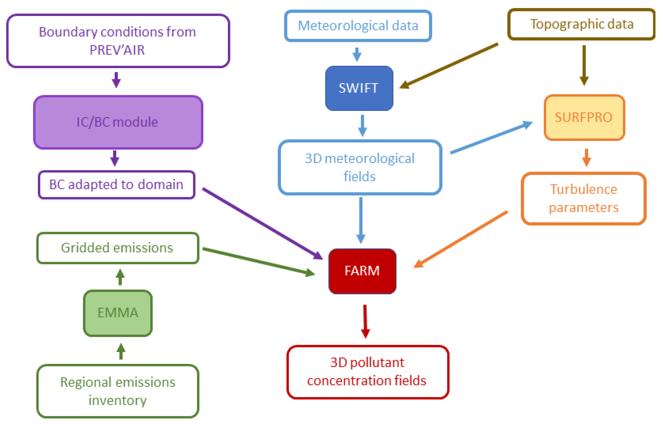
The CTM chain used in this study is based on the flexible air quality regional model (FARM, http://www.farm-model.org, accessed on 22 June 2021), a 3D Eulerian model accounting for transport, chemical conversion, and deposition of atmospheric pollutants (e.g., [60,61,62]). The system relies on additional data provided by emission inventories (Section 3.3.1), considering both local (i.e., within the boundaries of the domain) and remote sources (“boundary conditions”), and by a meteorological model coupled with a tool for the estimation of the turbulence parameters (Section 3.3.2). A scheme of the simulation chain is provided in Figure 2.

FARM (version 4.7) can process air pollutant emissions from both area and point sources by considering transport and gas-phase chemical transformations [63]. Primary and secondary particle dynamics, and their interactions with gas-phase species, include nucleation, condensational growth, and coagulation processes [64]. Further details on the FARM working principles are provided elsewhere (e.g., [43,44]).

In this study, the modelling system is run on a 110 × 70 km${}^2$ domain, roughly corresponding to the Aosta Valley (Figure 1b), on a 1-km spatial grid, and at 1-h time steps. A total of 16 different vertical levels (from the surface to 9290 m) are considered. Two runs relative to 2020 (each one over 366 days) are performed. The first simulation incorporates emissions from the previous year (2019, assuming no relevant variation compared to, e.g., 2015–2018) as the reference scenario, while in the second one, curtailed emissions are used, as explained in the next section (lockdown scenario). The same meteorological fields from 2020 (Section 3.3.2) are kept in both runs.

3.3.1. Emissions and Their Modifications during the Pandemic

The regional emission inventory of the Aosta Valley is fully set up and maintained in-house and is detailed according to the 11 conventional categories listed in Section S3. The inventory includes the estimated emissions of several atmospheric pollutants, such as NO${}_x$, PM, NH${}_3$, heavy metals, and of the most important greenhouse gases (CO${}_2$, CH${}_4$, N${}_2$O).

These emission data are pre-processed by the emission manager (EMMA, http://doc.aria-net.it/EmissionManager, accessed on 22 June 2021) and interpolated to every cell of the domain grid $\overrightarrow{x}$. The modulation of the mass emissions $E_i(\overrightarrow{x},t)$ is described using a temporal profile for each air pollutant i based on the number/power $A_j(\overrightarrow{x},t)$ of the considered emitter j and a set of estimated emission factors $F_{ij}$ (expressed as mass in relation to the activity index A), according to the following formula:

$$E_i(\overrightarrow{x},t)=\sum _j{A}_j(\overrightarrow{x},t)·F_{ij}$$

(2)

The emission factors (for every type of source j and pollutant i) are generally those reported in the atmospheric emission inventory guidebook [65], unless more specific or up-to-date information is applicable based on the expertise of the operator and knowledge of the processes acting on a regional scale.

As anticipated, two distinct scenarios—a reference (2019) and a curtailed (2020) one–are used with differences in emissions by the industrial and road transport sectors. The other sources, such as agriculture and waste, are left unchanged. Among them, domestic heating in 2020 is assumed to not be impacted by the restrictions. Notably, methane consumption from January to April (2019 and 2020) provided by the national methane pipeline society (SNAM) are compared, resulting in about the same values (yearly average difference < 1%). Emissions from the steel mill in Aosta, which is the only relevant industrial establishment in the region, are modulated based on flume flows collected at the main chimney. This is particularly important from March to mid-April 2020 (period 2 in Table 2), when the industrial plant is closed due to the complete lockdown. Finally, variations in international and local road traffic are quantified based on vehicle flow measurements from several sources, such as data provided by the administration of the Mt. Blanc tunnel, specifically designed webcams on motorway and regional roads, and traffic counters on urban roads (Section 2.2). Traffic reductions–reaching nearly 100% through the Mt. Blanc tunnel in P2–P3, 90% on the motorway, and 75%–80% on the other roads (notably, in the Aosta urban road network)–likely represent the most relevant effect of the confinement measures on emission abatement in the Aosta Valley.

The boundary conditions, which were used to estimate the air mass exchange from outside the borders of the FARM domain, are prepared starting from the daily simulations elaborated on a continental scale with the CHIMERE model [66] and operationally made available by the Prev’Air service (http://www.prevair.org, accessed on 22 June 2021). Such boundary conditions, provided by the regional environmental protection agency of Piedmont for year 2020, are used as-is for both (lockdown and business-as-usual) emission scenarios since they are not released separately for real and counterfactual conditions. Indeed, an accurate modulation of the national and continental emissions and notably, their anthropogenic fraction would require an extremely large effort, which is out of the scope of this work and would anyway result in considerable uncertainties (e.g., effect of regulations on secondary air pollutants). As a consequence, the observed changes in concentrations resulting from FARM simulations describe the effect from local emissions only.

3.3.2. Diagnostic Meteorological Model and Turbulence Pre-Processor

SWIFT [67,68], a variational 3D wind model, is invoked to produce a mass consistent wind field over complex terrain at local and regional scales starting from wind measurements from a meteorological network (temperature and humidity fields can be interpolated too). The model uses the first Navier–Stokes equation and the mass conservation to account for the effect of terrain on the flow structure. Here, we use data every 30 min from 25 meteorological stations in the Aosta Valley. A turbulence and deposition pre-processor (surface-atmosphere interface processor, SURFPRO) computes the gridded fields of the planetary boundary layer turbulence scaling parameters, horizontal and vertical eddy diffusivities, and deposition velocities according to land cover type, atmospheric circulation conditions, and characteristics of the different chemical species.

3.4. Aerosol Source Apportionment

To accurately identify the particle emission sources and their modulations over the course of 2020, we process the aerosol chemico-physical properties available at some of the sampling sites using the positive matrix factorisation (PMF) technique (Section 3.4.1) and the aerosol optical properties at the surface, taking advantage of the different spectral light absorption characteristics of fossil fuel and biomass burning components (Section 3.4.2).

3.4.1. Positive Matrix Factorisation

This technique [69,70] splits a multivariate series (e.g., a set of aerosol properties over time) into two matrices containing only non-negative elements, defining the strength and the characteristics of each source, respectively, in a similar way as already described in another context by Equation (2). Keeping the same formulation as in Section 3.3.1,

$$C_i\left(t\right)=\sum _j{A}_j\left(t\right)·F_{ij}$$

(3)

where $C_i\left(t\right)$ is, in this case, the mass concentration of element i at the receptor (either a chemical element or a size class, part of a multivariate data set), $A_j\left(t\right)$ is a measure of the activity of source j, and $F_{ij}$ is the source profile, i.e., a description of the emission type with reference to the available elements sampled. The purpose of PMF is to identify sets of elements varying together (within the same group), thus attributed to the same source, while the contribution of each source is temporally uncorrelated to the other. The US EPA PMF5.0 implementation [71] is here employed to factorise both the dimensional data set from the three Fidas200E optical particle counters, and the Aosta–downtown chemical characterisation. In the first case, the variables are the 64 dimensional classes measured at an hourly frequency (the results are then averaged at daily resolution), further weighted by a typical cut-off efficiency of the PM${}_{10}$ sampling head [44] to ensure comparability to measurements with common PM samplers. This “size-PMF” allows the different modes to arise more naturally than a subjective choice of the size classes, such as, e.g., PM${}_1$, PM${}_{2.5}$, or PM${}_{10}$. In the second case (“chem-PMF”), the considered variables are the chemical elements listed in Section 2.2, which are collected at daily resolution. Since the complete chemical characterisation is not available at the same time owing to the used schedule (Table 1), three different combinations based on the simultaneous information, i.e., anion/cation only, anion/cation together with coincident organic carbon analyses, and anion/cation with metals are possible [44]. However, in order to not duplicate information, we only analyse the last two data sets, i.e., the most complete ones. In particular, the series with levoglucosan and EC/OC (464 days) helps us to differentiate between biomass and non-biomass combustion processes, while the one with metals (856 days) allows us to assess the effect of the industrial lockdown on the air quality in Aosta–downtown. NO and NO${}_2$ from co-located measurements are additionally included in chem-PMF to facilitate the identification of local air pollution sources. For both decompositions, the number of factors for each data set is chosen based on physical interpretability of the resulting factors and the goodness of fit ratio to its expected value (Q/$Q_{exp}$) [71]. PM${}_{10}$ is considered a total variable, i.e., the contribution of each identified mode is calculated with respect to the measured PM${}_{10}$ mass concentration.

3.4.2. Optical Properties at the Surface

UV, visible, and near infrared aerosol light absorption coefficients are measured with the AE-33 aethalometer. Ambient concentrations of eBC are then retrieved using data obtained at 880 nm and known mass absorption cross section coefficients (MACs). In this study, site-specific MACs are experimentally determined using elemental carbon (EC) concentrations from PM${}_{10}$ samples collected at the same site. Our results indicate that the MAC at 880 nm at Aosta–downtown is 6.0 m${}^2$ g${}^{-1}$, i.e., lower than the default AE-33 value (7.77 m${}^2$ g${}^{-1}$) but in agreement with values reported for urban aerosols and externally mixed BC with little coating [72,73].

Afterwards, the measured eBC is apportioned into its fossil fuel (eBC${}_{ff}$) and biomass burning (eBC${}_{bb}$) contributions based on wavelength-dependent light absorption [74]. This method is critically sensitive to the AÅE assumed for fossil fuel and biomass burning (AÅE${}_{ff}$ and AÅE${}_{bb}$, respectively). Hence, the response of the “aethalometer model” is evaluated by varying AÅE${}_{ff}$ and AÅE${}_{bb}$ within a reasonable range [75]. The final coefficients are selected based on the results of the correlation analysis between the levoglucosan mass measured on site and the retrieved eBC${}_{bb}$. Notably, the optimal AÅEs are chosen so that the regression line has intercept close to zero, under the assumption that both biomass tracers are removed from the atmosphere at a similar rate. During an intensive measurement campaign in 2018, this analysis gave the values AÅE${}_{ff}$ = 1.1 and AÅE${}_{bb}$ = 2.2, which are used here.

4. Results

We start this section with an assessment of the meteorological situation in 2020 compared to the five previous years (Section 4.1). Then, we examine the air quality changes relative to the reference scenario for both gaseous pollutants (Section 4.2) and PM (Section 4.3) at the surface. In order to explain the weaker reduction of aerosol concentrations compared, e.g., to nitrogen oxides, both source apportionment techniques (Section 4.4) and vertical column amounts/profiles (Section 4.5) are considered.

4.1. Meteorological Context in 2020

We use the daily weather classification developed in one of our previous studies [44] based on the surface meteorological variables measured at the Aosta–Saint-Christophe station (chosen as the representative of the wind flows at the bottom of the valley) to compare the occurrence of different weather patterns in 2020 with the previous years. The results from the classification are illustrated in Section S4 together with some general comments. Here, we limit ourselves to a list of the meteorological features encountered in 2020 that are relevant to the present study:

–

P1 presents only few days with easterly winds, while westerly circulation is above average. The temperature in P1 during 2020 is also higher, on average, than the previous years;

–

P2, P3, and P4 in 2020 feature more days than average with easterly winds (indeed, 2020 holds the record of the last years in P2 and P4);

–

Days in P5 with persistent westerly flows are more frequent in 2020 than average, while the opposite occurs for easterly winds. The total precipitation amount is larger than average in Aosta and Donnas;

–

Days with westerly flows are fewer than average in P6 in 2020. Moreover, the temperature in Aosta in this period is lower than average. Thus, although precipitation is less abundant, snowfalls in Aosta are more frequent than average (about 9 days in 2020 compared to 1 day, e.g., in 2019 and 2018).

In addition to the local meteorological conditions, synoptical patterns leading to air pollution transport over the medium (e.g., from the Po basin) and long range (e.g., from the Sahara desert) must also be considered. The most relevant episodes occurring in 2020 are identified based on the examination of the ALC profiles, wind provenance, and back-trajectories [43,44]:

–

P1 is characterised by some episodes of advection of polluted air masses from the Po basin (for a total of 25 days, i.e., 37% of the time in the period). Saharan dust is also transported on seven days overall in this period.

–

P2 features an extraordinarily long series of transport episodes of fine particles from the Po basin (almost continuously from 14 March to 13 April, i.e., 88% of the days), according to the frequent easterly wind flows mentioned above, and mineral dust from Sahara (mainly floating at some km from the surface without settling on the ground but detected by the ALC and the sun/sky radiometer, Section 4.5). Within this period, moreover, we notice a remarkable and very unusual transport of dust particles from the area of the Caspian sea and Aral lake (e.g., [37]) between 28 and 30 March, leading to instantaneous PM${}_{10}$ concentrations $>50$ $\mathsf{\mu }$g m${}^{-3}$ in Aosta–downtown, with these particles being mostly concentrated in the coarse mode.

–

During P3, transport from the Po basin occurs for a dozen days (62%, according to the larger-than-usual frequency of easterly winds), with both fine and coarse particles involved (these latter likely still circulating from the previous long-range events).

–

More than 50% and about 45% of the days are affected by advection of fine and coarse aerosol from the Po basin in P4 and P5, respectively. In line with the 2020 increase in westerly winds in P5, the latter fraction is lower than average for the summer–autumn months, which, in 2020, feature a long sequence of events in September (19 days continuously) but almost no episodes in October.

–

Finally, in about 38% of the days in P6 the air quality in the Aosta Valley is impacted by the transport of fine particles from the Po basin, although easterly winds are too weak and intermittent to be detected by our automatic weather pattern classification, while dust is identified (but not at the surface) on 3 days only.

4.2. Changes in Surface Gaseous Pollutant Concentrations

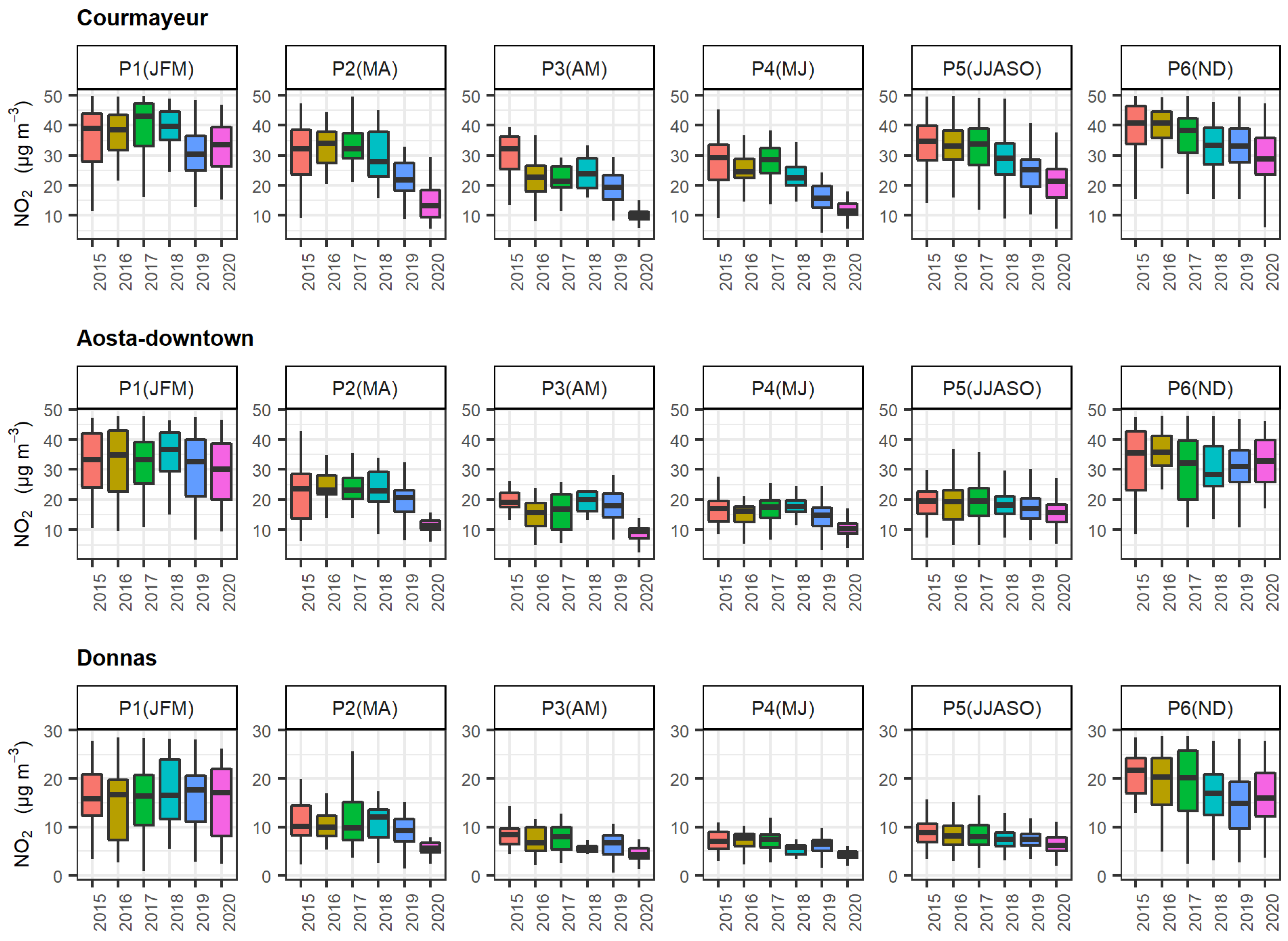
The statistical distributions of daily average gaseous pollutant concentrations in the different lockdown phases analysed in this study are represented in Figure 3 for NO${}_2$, as an example, and Figures S6 and S7 for NO and O${}_3$, respectively, in comparison with the previous years. Nitrogen oxides exhibit a rather sharp decrease everywhere in 2020 and during the whole year, especially in periods P2–P4, i.e., during the strict lockdown and the following confinement phase within the region. The NO${}_x$ concentrations observed in 2020 are even lower than the ones registered in 2019, a year characterised by weather patterns particularly favourable to air pollutant dispersion. As already noticed in the scientific literature (e.g., [20]), both the median of the concentrations and their variability decrease, owing to the weakening emissions and their periodic modulation. Changes in ozone, on the other hand, are much more limited.

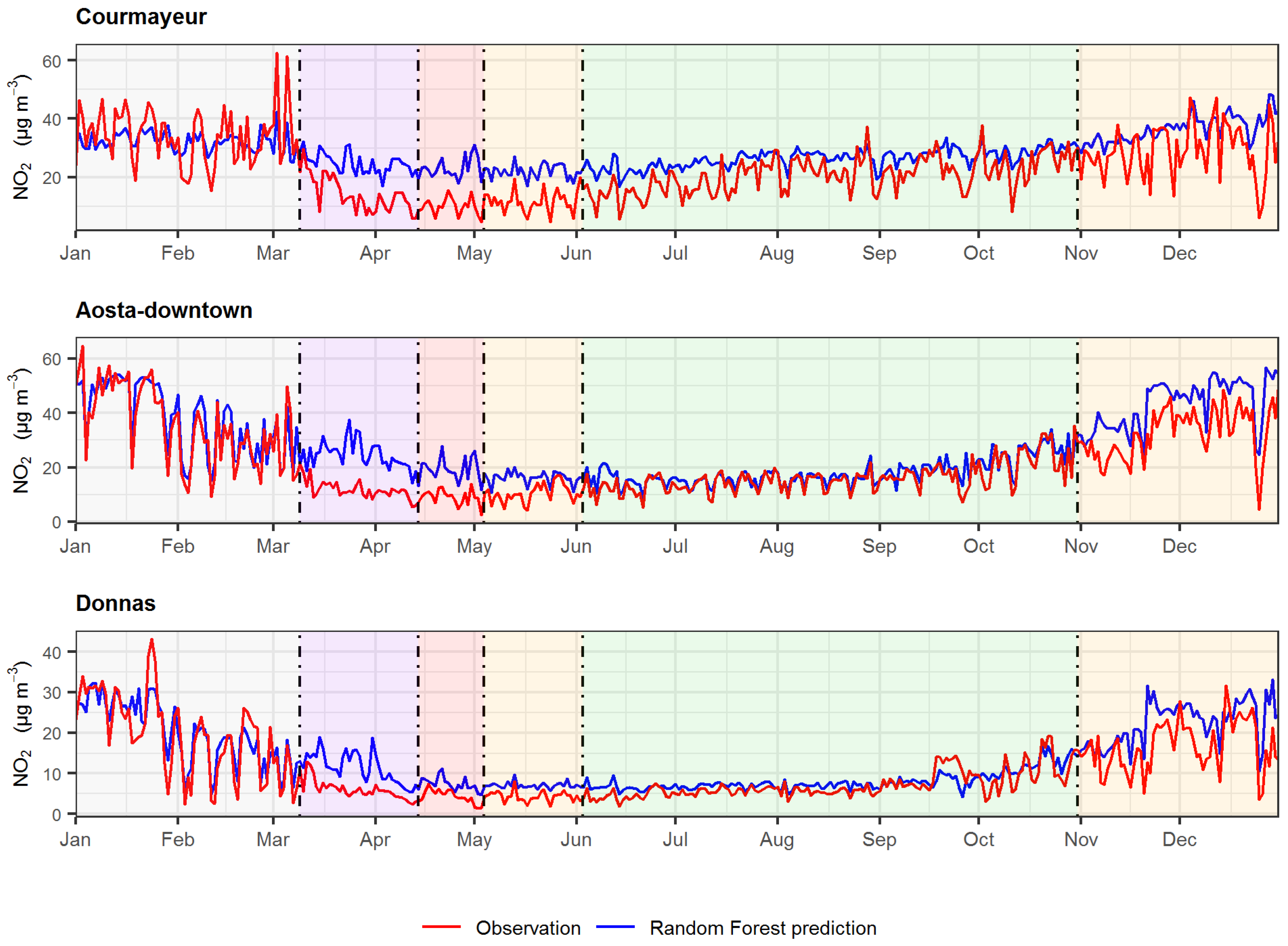
An even better detail can be captured by observing the seasonal evolution of the daily measured gas concentrations in 2020 and the output of the predictive statistical model, representing the counterfactual reference. These are shown in Figure 4 for NO${}_2$, as an example, and Figures S8 and S9 for NO and O${}_3$. An overall good agreement between the measured and predicted NO${}_x$ data sets can be noticed before the beginning of the restrictions in P1. An abrupt split of the curves occurs after the establishment of the confinement regulations in P2–P4 and again in P6. In Aosta–downtown and Donnas, the difference between the NO${}_x$ observations and the counterfactual scenario tends to decrease and vanishes in P5. Conversely, a negative offset persists in Courmayeur likely due to the influence of international road traffic, still 15%–20% lower than usual, and to the exceptional occurrence of westerly winds, not fully compensated by the random forest.

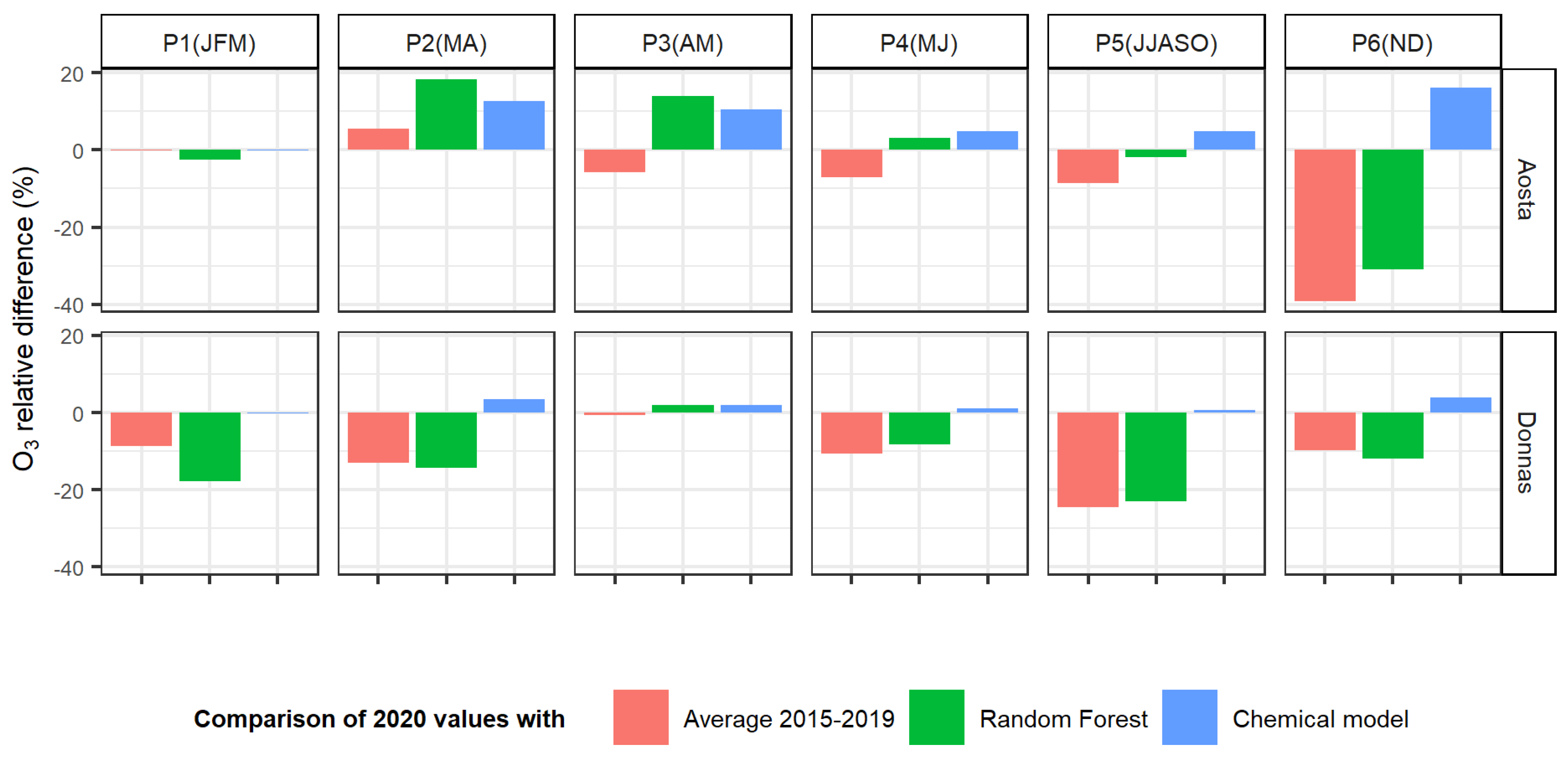
The results for O${}_3$ are less clear and more difficult to interpret. In P2–P3, we observe an increase in Aosta–downtown compared to the random forest prediction and a decrease in P2 in Donnas. A possible reason for this contrasting behaviour could be that reduced titration by NO leads to increased concentrations of ozone in the urban environment of Aosta, while reduced precursors contribute to the decrease at the Donnas rural station, as also found at other remote Italian sites [76]. However, in contrast to P2–P3, O${}_3$ concentrations slightly decrease in Aosta–downtown during the second lockdown in P6. This can be explained in the following way. Ozone production in winter due to photochemistry is negligible and the only phenomena contributing to the O${}_3$ increase in the Aosta Valley in winter are Foehn winds, which bring ozone-rich air masses from higher altitudes down to the surface. Since in 2020, westerly circulation was much weaker than the previous years in P6, the ozone concentrations are also lower than usual. However, it must be considered that O${}_3$ absolute concentrations are much lower in winter compared to P2–P3 (e.g., Figure S9), and the relative changes are probably not significant. Finally, it should be noticed that, in Donnas, the largest difference between the observed O${}_3$ concentrations and the ones predicted by the random forest occurs in P5. This is consistent with the overall O${}_3$ negative anomaly detected in northern Italy in summer 2020 [76], especially considering that Donnas is very close to the Po basin.

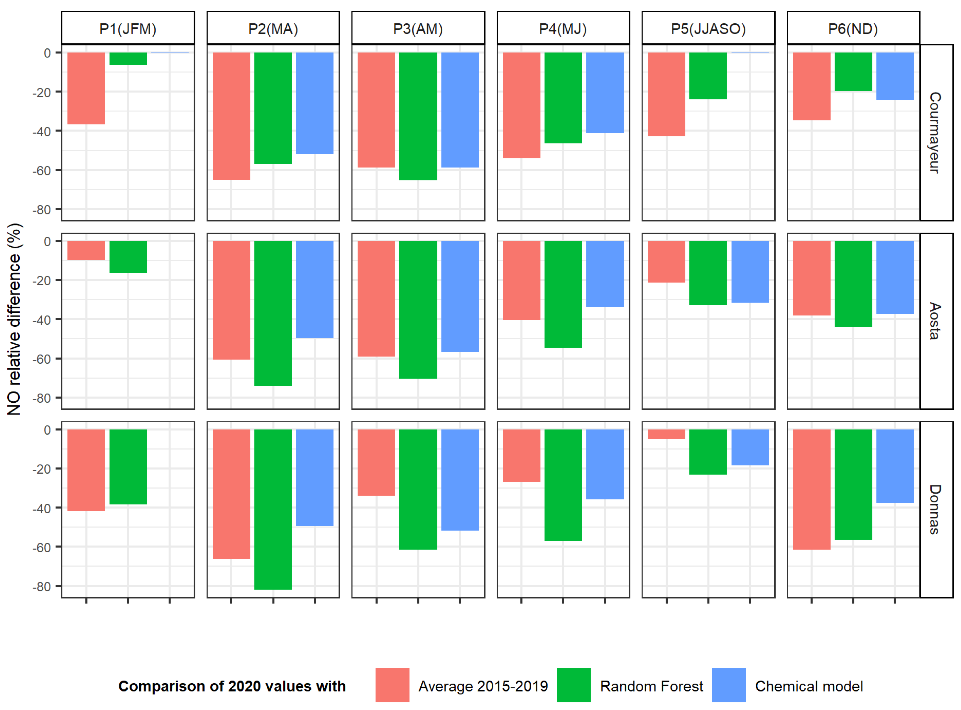
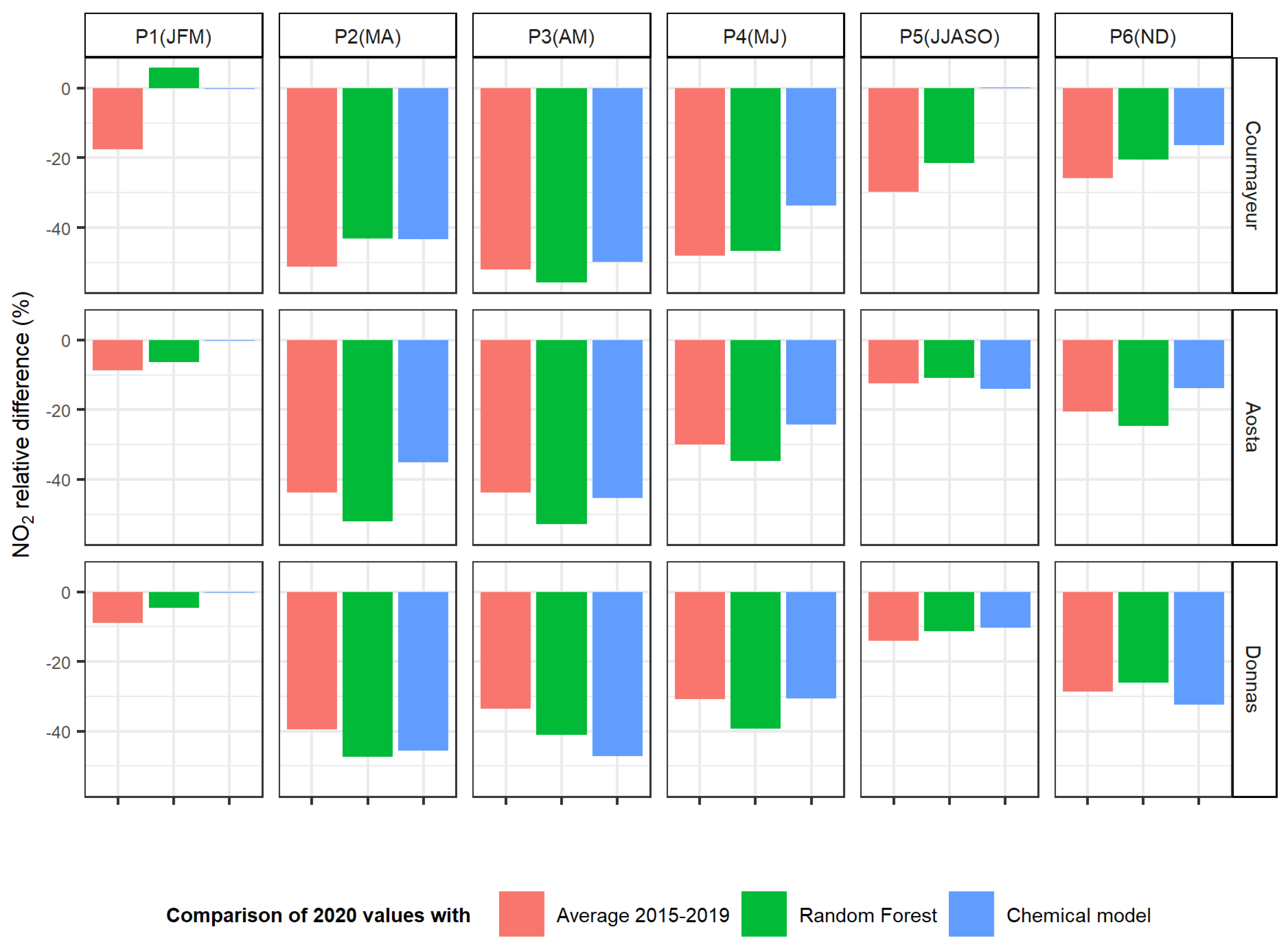
The reductions of gaseous pollutant concentrations estimated by all methods, including CTMs, are quantified and compared in Figure 5, Figure 6 and Figure 7 for NO, NO${}_2$, and O${}_3$, respectively. The reduction in NO concentrations with respect to the previous years’ average reaches −60% everywhere in P2, which is very homogeneous despite the wide range of absolute variations (−0.5 $\mathsf{\mu }$g m${}^{-3}$ in Donnas, −4.5 $\mathsf{\mu }$g m${}^{-3}$ in Aosta–downtown, and −9.1 $\mathsf{\mu }$g m${}^{-3}$ in Courmayeur), and also in P3 in Courmayeur (−5.9 $\mathsf{\mu }$g m${}^{-3}$) and Aosta–downtown (−3.7 $\mathsf{\mu }$g m${}^{-3}$). Values as low as −50% (−6.6 $\mathsf{\mu }$g m${}^{-3}$) in Courmayeur persist even in P4. For NO${}_2$, the decrease compared to the previous years is slightly weaker but still important, reaching −40% or even −50% in P2–P4 (e.g., −14.6 $\mathsf{\mu }$g m${}^{-3}$ in Courmayeur, −9.0 $\mathsf{\mu }$g m${}^{-3}$ in Aosta–downtown, and −3.9 $\mathsf{\mu }$g m${}^{-3}$ in Donnas). The new decrease in P6, at the end of the year, amounts to about −40% to −60% for NO (−9.5 $\mathsf{\mu }$g m${}^{-3}$ in Courmayeur, −17.4 $\mathsf{\mu }$g m${}^{-3}$ in Aosta–downtown, and −4.4 $\mathsf{\mu }$g m${}^{-3}$ in Donnas) and to −20% to −30% for NO${}_2$ (−10.2 $\mathsf{\mu }$g m${}^{-3}$ in Courmayeur, −8.5 $\mathsf{\mu }$g m${}^{-3}$ in Aosta–downtown, and −6.7 $\mathsf{\mu }$g m${}^{-3}$ in Donnas). As already mentioned, a remarkable reduction of about −40% (−7.9 $\mathsf{\mu }$g m${}^{-3}$) for NO and −30% (−8.8 $\mathsf{\mu }$g m${}^{-3}$) for NO${}_2$ relative to the average of the previous years is also found during P5 in Courmayeur.

The predictive statistical model provides similar results to the anomalies relative to the previous years, even enhancing the NO${}_x$ reductions found in periods P2–P4. Hence, the weather-compensated NO changes reach −80% (−1.2 $\mathsf{\mu }$g m${}^{-3}$) in Donnas in P2 and −70% (−8.3 to −6.1 $\mathsf{\mu }$g m${}^{-3}$) in Aosta–downtown (P2–P3), with still important decreases in P4 and P6, and the NO${}_2$ reductions touch −50% everywhere (−13.0 $\mathsf{\mu }$g m${}^{-3}$ in Courmayeur, −12.6 $\mathsf{\mu }$g m${}^{-3}$ in Aosta–downtown, and −5.4 $\mathsf{\mu }$g m${}^{-3}$ in Donnas). These enhanced reductions (with the exception of O${}_3$), especially in Aosta–downtown and Donnas highlight that local meteorology alone, in 2020, would shift the air pollutant concentrations towards higher values, i.e., contribute to degrade the air quality. Instead, due to the large reduction in pollutant emissions owing to the lockdown, the influence of meteorology is compensated, and net decreases are generally observed. The calculation of the difference between the random forest output and the previous years’ average provides an estimate of the effect by the meteorology. The results are shown for period P2 as an example in

Table 4. The effect of local meteorology on air pollutant concentrations measured at the surface during period P2 (March–April 2020), obtained as the difference between the random forest prediction for 2020 and the previous years’ average.

Station	NO (%)	NO${}_2$ (%)	O${}_3$ (%)	PM${}_{2.5}$ (%)	PM${}_{10}$ (%)
Donnas	88.9	16.6	0.4	–	8.2
Aosta–downtown	51.5	17.7	−11.3	25.1	20.2
Courmayeur	−17.8	−13.5	–	–	−2.7

. NO is the pollutant most influenced by local meteorology. NO concentrations would have increased by up to 90% in Donnas and by more than 50% in Aosta due to weather effects if the confinement measures had not occurred. The impact of meteorology on NO${}_2$ concentrations is lower than on NO and comparable in both Donnas and Aosta–downtown (17%–18%). Interestingly, in Courmayeur the influence of meteorology is opposite to that at the other stations, likely because of different weather regimes. Finally, the influence on O${}_3$ strongly depends on the site for the reasons explained earlier in the text.

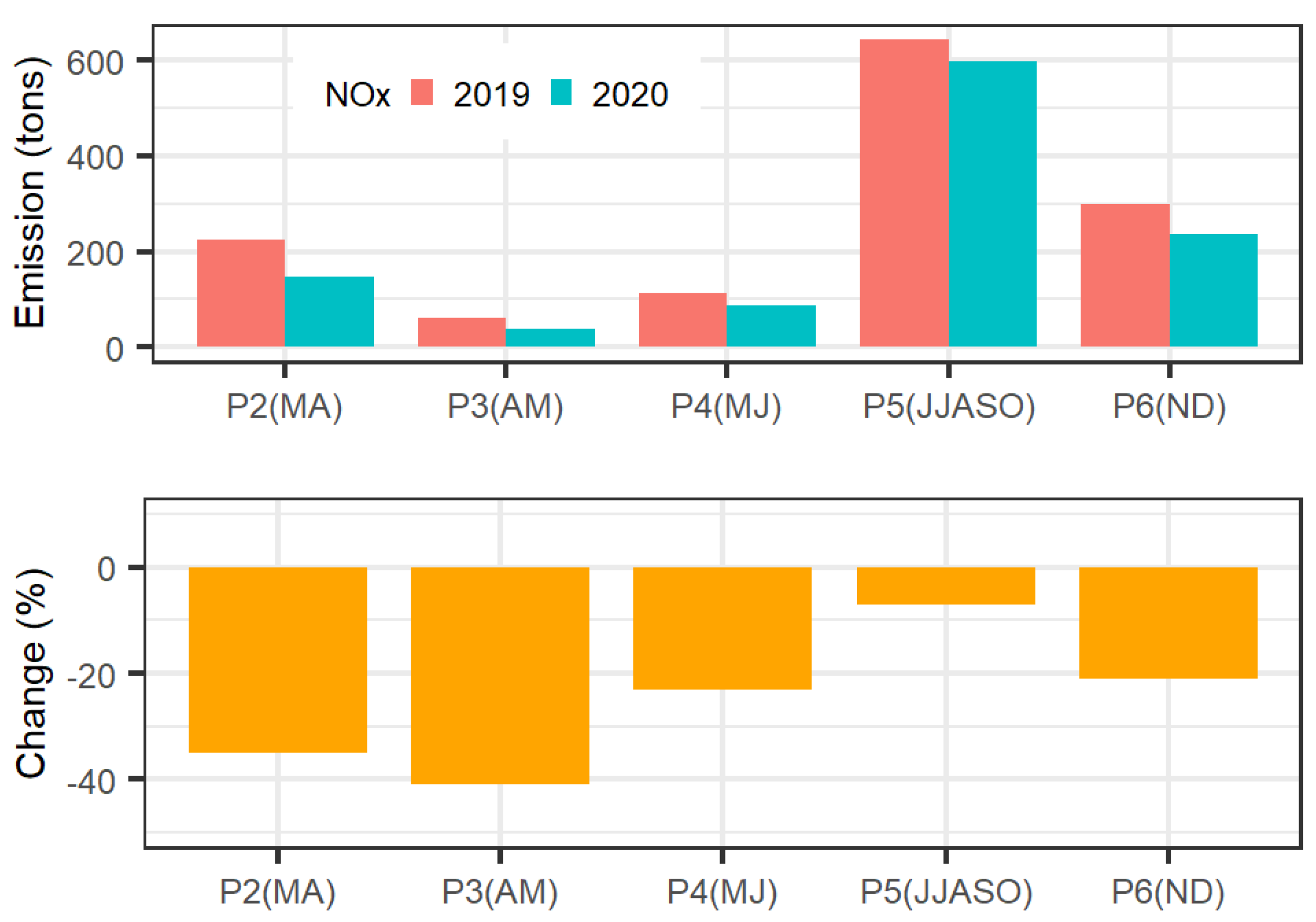
The CTM follows the effect of the lockdown on NO${}_x$ rather well, as already outlined by the predictive statistical model, with differences generally within 10%–20% to this latter. A few exceptions, with deviations larger than 20%, are visible in Donnas (P1–P2, and P4), in Aosta (P2 and P4), and in Courmayeur (P5). However, it should be kept in mind that NO${}_x$ concentrations are very low in the summer and that the complex orography (e.g., in Courmayeur, in the vicinity of the Mt. Blanc massif) could lead to inconsistencies between the CTM and measurements at the bottom of the valley. Overall, the CTM responds closely to the reductions of NO${}_x$ emissions provided by the inventory, which are represented in Figure 8 (notice that our inventory only includes NO${}_x$ emissions, which are partitioned at a second stage into NO, NO${}_2$, and O${}_3$ by FARM). The reductions amount to 35%–40% in P2–P3 and to 20% in P4 and P6, on average, in the Aosta Valley. The results for O${}_3$ are the most divergent ones, and the various methods show changes differing in both magnitude and sign. They highlight the challenge of interpreting and modelling the behaviour of this secondary compound depending on both meteorological and complex chemical mechanisms. The relative differences, however, are generally within 20%, which approaches the uncertainty of all used techniques, with the exception of P5 in Donnas and P6 in Aosta (these cases were already discussed above). Since FARM only accounts for changes in local emissions, it responds to the decreasing NO${}_x$ with an increase in O${}_3$.

To provide an example of the gaseous pollutant evolution over the whole domain and not only at the selected stations, a map of the differences between the simulated NO${}_2$ surface concentrations for the curtailed and reference scenarios in each period is presented in Figure S10.

4.3. Changes in Surface PM Concentrations

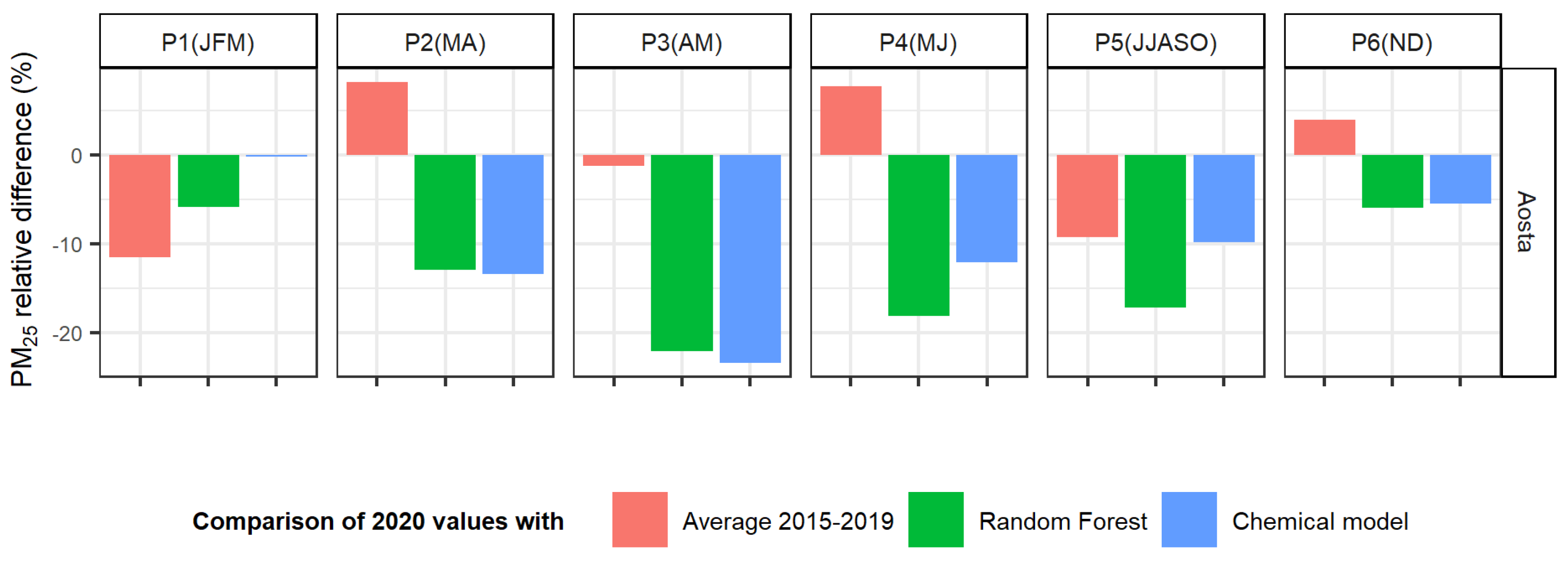
Surface PM concentrations in 2020 and in the previous five years are plotted in Figures S11 and S12. Even at first glance, similar year-to-year modulations at different stations can be seen, which are the result of large-scale weather patterns [44] and long-range aerosol transport affecting different sampling sites in about the same way. For example, minimum PM concentrations are found in 2019 due to the aforementioned particular meteorological conditions in that year.

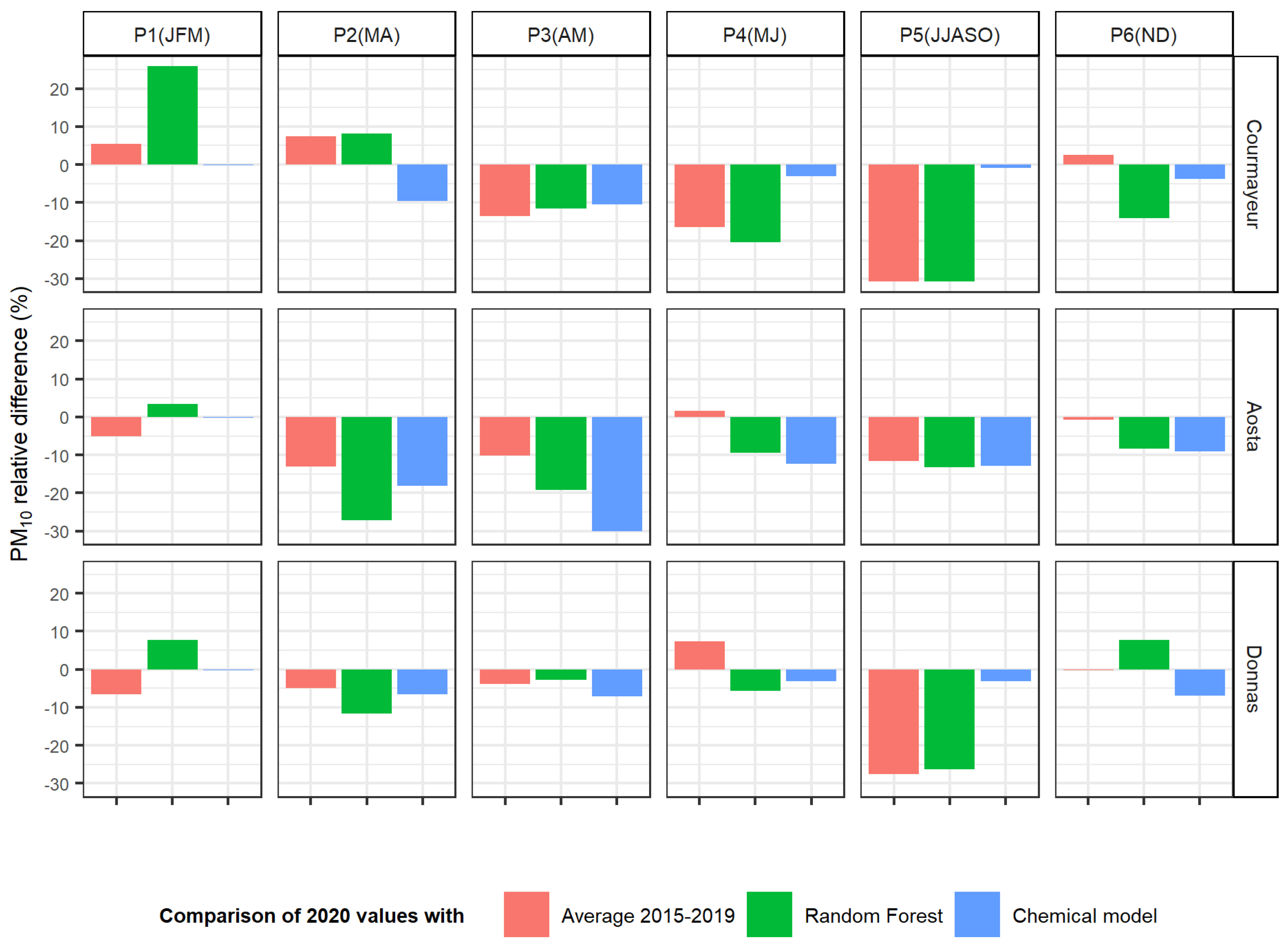
Figure 9 and Figure 10 provide a more quantitative view of the relative changes in 2020 with respect to the reference/counterfactual scenarios. One of the most striking features is the fact that, compared to the previous years’ average, PM${}_{2.5}$ in Aosta–downtown increases during the lockdown periods (by about 9–8% in P2 and P4, i.e., 0.9–0.5 $\mathsf{\mu }$g m${}^{-3}$, and by 4% in P6, i.e., 0.7 $\mathsf{\mu }$g m${}^{-3}$), while PM₁₀ decreases. This shows that the fine and coarse PM fractions have different sources and are subjected to different atmospheric processes. In particular, aerosols with a size between 2.5 and 10 $\mathsf{\mu }$m decrease by 50% in P2 (not shown) compared to the 2015–2019 average, i.e., about 3 $\mathsf{\mu }$g m${}^{-3}$, and contribute in a substantial way to the observed PM₁₀ reductions. However, if meteorology is taken into account with the predictive statistical model (Figures S13 and S14), the net effect of the restrictions on PM${}_{2.5}$ concentrations becomes negative (down to −22%, or −1.8 $\mathsf{\mu }$g m${}^{-3}$ in P3), while the PM₁₀ reductions already found with the anomaly calculation are generally enhanced (thus reaching, e.g., −27%, or −5.4 $\mathsf{\mu }$g m${}^{-3}$, in Aosta in P2). Indeed, from Table 4, we can notice that, in P2, local weather plays a major role on PM surface concentrations, especially in Donnas and Aosta–downtown. This could partially account for medium-range air mass transport, which is also related to the local weather conditions. As opposed to P2, in P1, the statistical model shifts the observed changes to (more) positive values, notably in Courmayeur. Based on the analysis of volume size distributions in Courmayeur (Section 4.4), the most likely explanation is the influence of dust transport and deposition (not included in the random forest parametrisation), coupled with weather conditions normally leading to a reduction of PM₁₀ concentrations. On the other hand, in P5, the two methods show remarkable agreement, especially in Courmayeur and Donnas where the largest reductions in 2020 are seen. This reduction may be due to weaker long-range transport of aerosol compared to average (Section 4.5). In this case, the evaluation of changes with the predictive statistical model is close to the anomaly calculation, as long-range transport is not included in the random forest. Conversely, since the CTM boundary conditions are the same for both the reference and perturbed scenario, the reduction due to the cleaner conditions in P5 is not reproduced by FARM, which only accounts for variations of local emissions. Moreover, the overall picture is rather consistent with the reduction in PM emissions according to the regional inventory (Figure S15), but aerosol concentrations appear to be more perturbed by transport dynamics than gaseous pollutants.

A spatial representation, over the whole domain, of the differences between the simulated PM₁₀ surface concentrations with the curtailed and reference scenarios in each period is presented in Figure S16.

4.4. Aerosol Source Apportionment

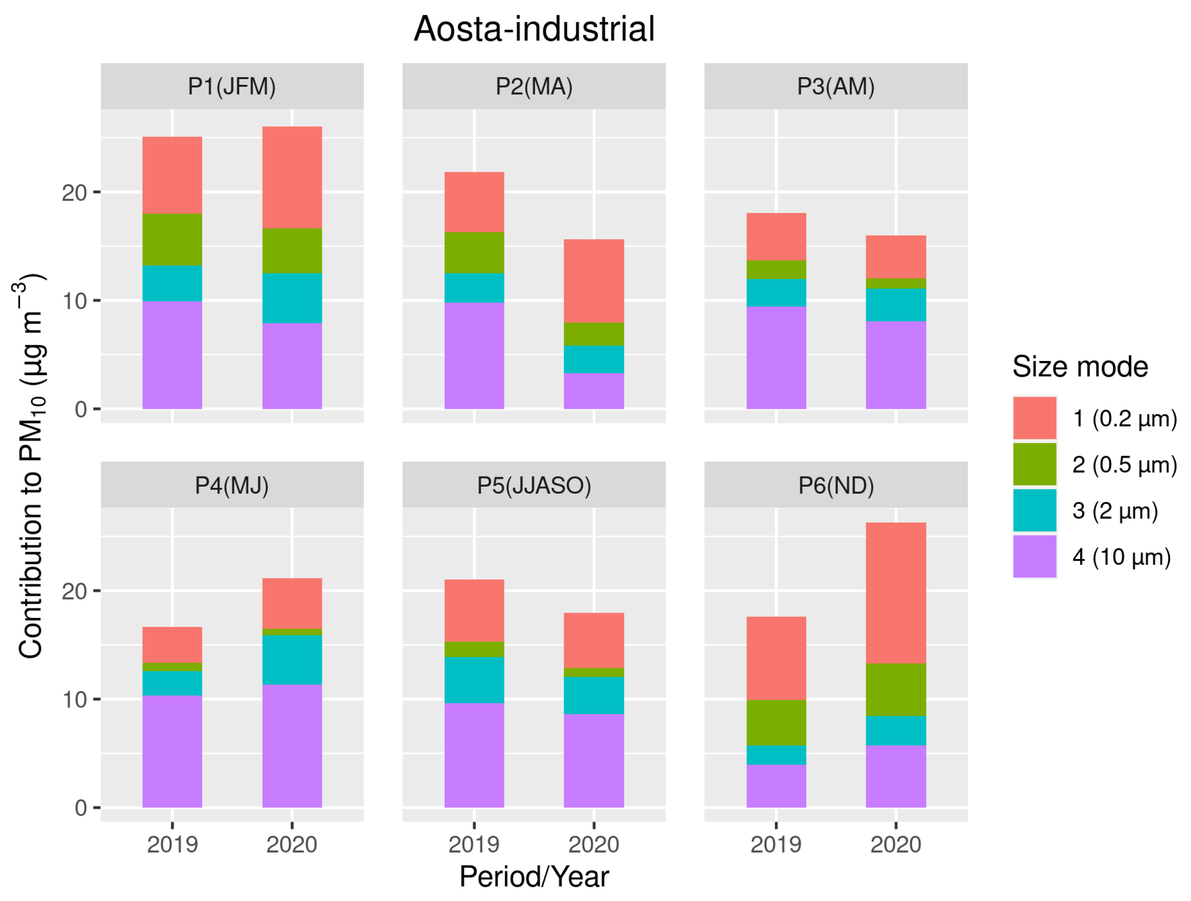
Four variation modes can be very clearly identified from size-PMF and are able to reconstruct the PM₁₀ concentration with a correlation index of 0.995, negligible offset (0.3 $\mathsf{\mu }$g m${}^{-3}$), and slope of 0.98. They consist of two fine modes (centred at about 0.2 and 0.5 $\mathsf{\mu }$m, respectively) and two coarse modes (at about 2 and 10 $\mathsf{\mu }$m). These are discussed in detail in Section S7 (Figures S17–S20). The size-PMF output is shown in Figure 11 for the Aosta–industrial station and in Figures S21 and S22 for Courmayeur and Aosta–downtown/Saint-Christophe. Although the size-PMF series are not long enough to allow us compare the 2020 anomaly with a longer-term average, we can still point out some microphysical characteristics of the aerosol in the Aosta Valley. First, fine particles (modes 1–2) are significant contributors to the total mass at all sites. Since their origin is both local and remote, this highlights the importance of monitoring and accounting for air mass transport, notably in the wintertime lockdown periods (P2 and P6). Likewise, owing to the decrease in easterly winds in P5, the contribution of fine particles, and even of the third mode (mineral dust), is lower than usual in that period. Aosta–industrial (Figure 11) represents an interesting case, witnessing in P2 (i.e., when the industrial plant is closed) a remarkable reduction of the coarse (mode 4) fraction, which is mainly coming from fugitive emission from the steel mill and, to a lesser extent, from car traffic. This is particularly interesting since, as already noticed in Section 4.3, a large contribution to PM reductions in Aosta–downtown in P2 (compared to the 2015–2019 average) comes from the 2.5–10 $\mathsf{\mu }$m size range (further insights are provided by chem-PMF). As soon as the steel mill resumes normal operation, the coarse particles increase again. Mineral dust is especially important in P3 in 2018 (from data collected in Courmayeur and Aosta–Saint-Christophe), which explains the large PM₁₀ concentrations in that period and year. As a final remark, coarse particles from de-icing road salt are very important at the Courmayeur traffic station in P1 and P6 and in Aosta in P6 in 2020 since this last winter was particularly snowy.

Several factors emerge from chem-PMF in Aosta–downtown depending on the considered variable subset: six factors are found from the decomposition using anion/cation, EC/OC, and levoglucosan (Figure S23), while seven factors arise when metals are included (Figure S24). These are further discussed in Section S7. All chem-PMF factorisations are able to reconstruct the PM₁₀ series with a correlation coefficient > 0.94 and only few swaps.

From the first factorisation, we show the evolution of non-biomass and biomass combustion processes in Figure 12. An almost total reduction of the first mode in the confinement periods (P2–4 and P6) in 2020, compared to the previous years (average from 2018 to 2019, for this data set), is visible, which can be assigned unambiguously to the reduction of traffic. Furthermore, notice a minor reduction during P1, which is likely due to higher temperatures and less domestic heating in 2020. Conversely, biomass burning shows a slight increase in P2 and a large increase in P6. However, when normalised to the total PM${}_{2.5}$ concentration (Figure S25), we see that this mode actually decreases (in P2) or does not change (in P6) in percentage compared to the previous years, indicating the more important influence of meteorology and air mass transport, as already found using the random forest technique in Section 4.3 for PM${}_{2.5}$ and PM₁₀. These conclusions are additionally supported by the optical source apportionment. Figure S26 shows that, despite the reduction of absolute eBC concentrations (and notably, their peak values) in P2 and P6 due to mobility restrictions, the ratio eBC${}_{ff}$/eBC is only marginally (by about −10%) affected and is still shifted to higher fossil fuel ratios. Hence, the role of biomass burning in counterbalancing the PM reductions during the confinement period is rather limited in Aosta–downtown compared to what has been hypothesised in other Italian regions [26,31]. However, in smaller villages of the Aosta Valley, where wood combustion is a more common practice, the importance of biomass burning emission may be greater.

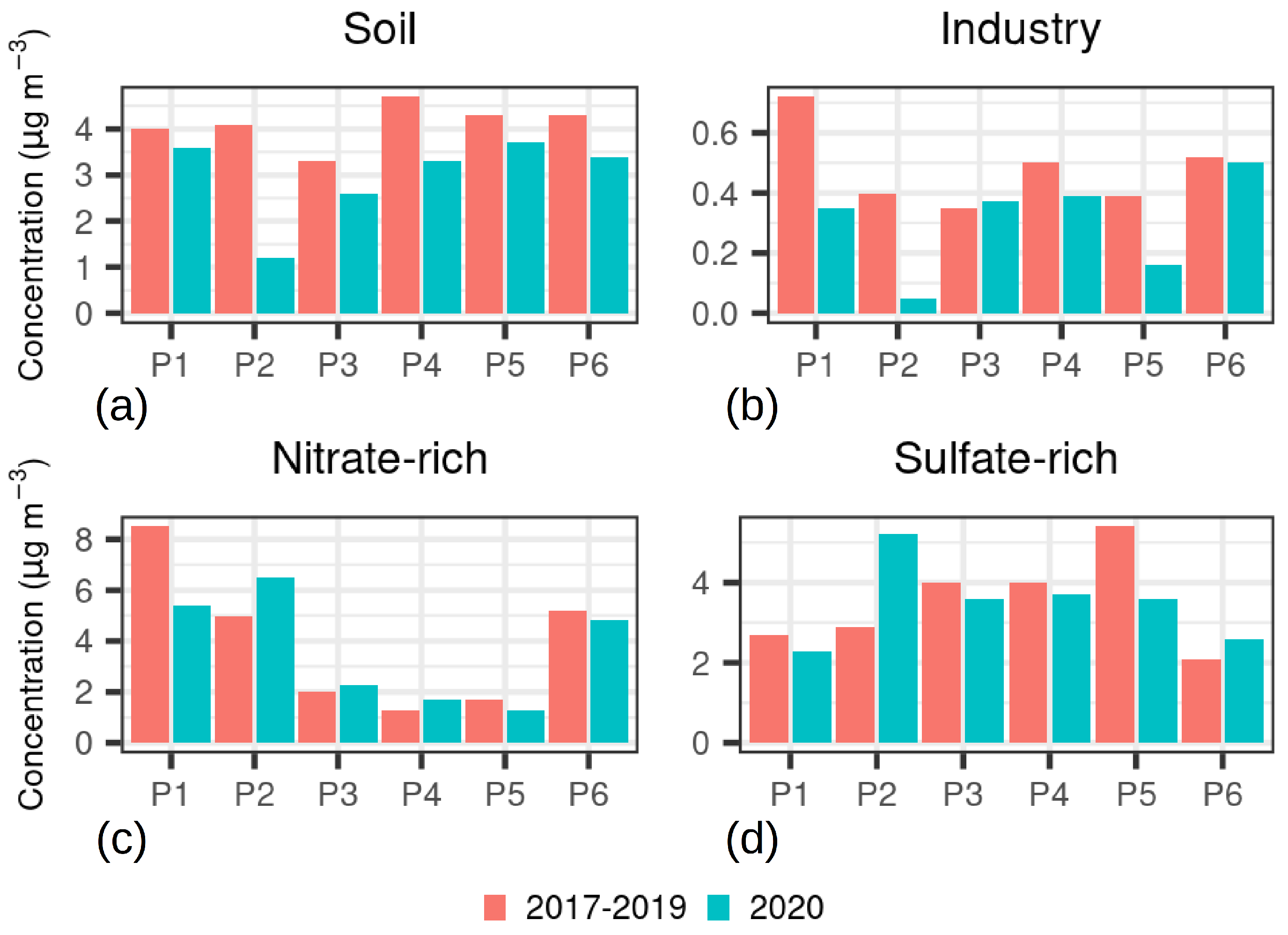
The soil mode shows an important reduction in P2 compared to the 2017–2019 average (Figure 13a), as well as a general decrease during the whole year due to both a decrease in the sources and the meteorological conditions (e.g., in P5). This decrease in P2 of about 3 $\mathsf{\mu }$g m${}^{-3}$, which is very consistent with the same changes in the PM${}_{2.5-10}$ fraction found in Section 4.3, is likely connected to the traffic reduction and to the shutdown of the steel mill. Indeed, it is worth noticing that crustal elements, such as Ca and Mg, may be connected with both resuspension by traffic/wind and emission from the industry. For example, oxides of Ca, Si, and Fe originate as slags from the electric arc furnace employed in the steel mill. Moreover, Ca, Si, Al, and Mg oxides form from refining treatments in the ladle furnace. These elements are present in the coarse fraction of fugitive emissions from the industrial plant and are believed to contribute to the “soil” mode at the Aosta–downtown station. Thus, resuspension and fugitive emissions from industry likely represent the missing source in the 2.5–10 $\mathsf{\mu }$m size range contributing to the reduction of the PM mass concentration in P2 in 2020. The closure of the industrial plant also reverberates on the metal concentration in Aosta–downtown, as apparent from the chem-PMF “industry” mode, driven by heavy metals (Figure 13b). Interestingly enough, although the concentrations of Cd and Pb completely drop at the Aosta–industrial station, the PMF mode rich in Cd and Pb (in Aosta–downtown, not shown) does not decrease relevantly, possibly indicating an additional source in the city. A secondary minimum in the “industry” mode occurs in P5, likely owing to the decreased activity of the steel mill in summer 2020 and to meteorological conditions unfavourable to the detection of industrial emissions at the Aosta–downtown station. The sum of the traffic, soil, and industrial modes in P2 (2020) is 4.2 $\mathsf{\mu }$g m${}^{-3}$ lower than the corresponding average from the previous years.

As opposed to the soil and traffic modes, the two modes rich in nitrate and sulfate, respectively, remarkably increase in P2 compared to the previous years (Figure 13c,d). Their sum in 2020 is 3.7 $\mathsf{\mu }$g m${}^{-3}$ larger than the corresponding value from the previous years. This increase is almost certainly due to the anomalous frequency of easterly winds in the same period in 2020 (Section 4.1), which bring polluted air masses from the Po basin to the Aosta Valley. However, an increase in secondary aerosol production in the urbanised source regions of the Po basin due to the enhanced oxidising capacity of the atmosphere (e.g., [77]) cannot be excluded. Finally, meteorology—and, notably, more frequent westerly winds in 2020—is also the most reasonable explanation of lower-than-usual concentrations of fine particles during P5.

4.5. Vertical Profiles and Column Amounts

Since P3 is characterised by higher-than-usual precipitation and cloudiness (Section 4.1), which hampers retrievals with both the sun/sky radiometer and the ALC, and since P3 is rather short, in this final section, we merge P2 and P3 into a single period.

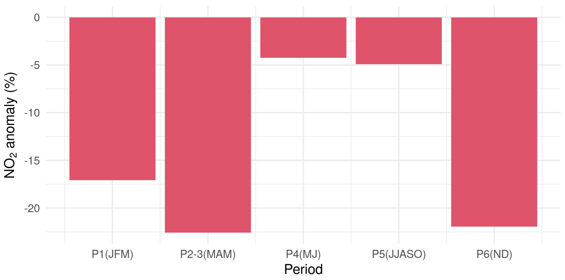
The 2020 anomaly in the total NO${}_2$ vertical column detected by the Brewer spectrophotometer is shown in Figure 14. This closely resembles the results obtained at the surface in Aosta–downtown (Figure 6). In particular, the NO${}_2$ maximum reductions in P2–3 and P6 also seen at the surface are correctly reproduced over the column, albeit with different intensities. This is to ascribe to the fact that stratospheric NO${}_2$ (unperturbed by surface changes) is at its maximum in the summer and represents a relevant part of the vertical column over the Aosta Valley, while the tropospheric column dominates the total NO${}_2$ VCD in the winter. This is likely the reason why, in P4, we do not detect large variations compared to the previous years in contrast to surface measurements. Finally, NO${}_2$ VCDs decrease in P1. This is also noticed in surface concentrations and could be attributed to reduced NO${}_x$ emissions by domestic heating systems, owing to higher temperatures (Section 4.1), and to decreased easterly winds possibly transporting some NO${}_2$ in the tropospheric column [44].

The relative anomaly in PM concentrations retrieved by the ALC along the vertical profile is depicted in Figure 15, which reveals some interesting details. First of all, in almost every period, the aerosol load in the elevated layers above the surface is larger in 2020 than in the previous years, likely due to increased long-range particle transport (Section 4.1). Only P5 proves to be a relatively clean period in 2020 compared to the average, which is the reason for the remarkable PM reductions detected at the various stations in May and June 2020 despite unperturbed emissions (Figure S15). This yearly evolution along the vertical column is fully confirmed by the aerosol optical depth from the sun/sky radiometer (Figure S27), showing larger-than-usual AODs in all periods except P5. Once again, this analysis demonstrates that long-range transport can interfere and should be accounted for in the determination of the effects from varying surface emissions and that column or profile measurements are effective in identifying such situations. Even more interestingly, in the periods affected by the lockdown restrictions (P2–3, P4, and P6), we notice, from Figure 15, some reductions of the PM mass concentration in the layers close to the ground despite the overall increase in the aerosol load in the atmosphere. These reductions are mostly concentrated during the day and notably during the rush hours when the greatest decreases of aerosol emissions at the surface are expected due to the confinement measures. The diurnal valley convection could then favour the mixing of this cleaner air, with effects visible up to about 1000 m a.s.l., i.e., some hundreds of metres above the surface. At higher altitudes, but still within the mixing layer (e.g., 1000–1500 m a.s.l.), the mean absolute increase in the aerosol mass detected by the ALC in P2 (2020) compared to the average of the previous years is about 5 $\mathsf{\mu }$g m${}^{-3}$. This value is very consistent with the changes in secondary aerosol concentrations detected by chem-PMF at the surface (3.7 $\mathsf{\mu }$g m${}^{-3}$, Section 4.4) and attributed to transport from the Po Valley. The contribution of dust particles and aerosol hygroscopicity, which is included in the ALC retrieval but not in the estimate of the secondary aerosol concentrations, could also lead to the slightly larger estimate from the profiles compared to chem-PMF, although the uncertainties of both methods do not allow further investigations.

5. Discussion and Conclusions

The present study analysed the effect of the COVID-19 confinement regulations on air quality in the northwestern Alps. Five sites in the Aosta Valley were selected and characterised by different environmental conditions. Data from 2020 (from winter to winter) and the previous years (back to 2015, depending on the considered data set), collected with different techniques both at the surface and in the vertical column, were studied, and some of them were compared to the output of statistical and deterministic models.

Based on the research questions mentioned in the introduction, we can now draw the following conclusions.

-

Q1–3: Changes in air pollutant concentrations, their magnitude, sign, and sources. At all examined stations, even the rural ones, relevant changes in air quality resulting from the confinement regulations can be identified. The largest variations occur for NO${}_x$ due to curtailed emissions from vehicular traffic. NO decreases by 60%–80% in March–May 2020 and by 20%–60% in November–December, depending on the site, while NO${}_2$ decreases slightly less, by about 40%–50% and 20%–25% in the two periods, respectively. These values agree with the results from previous studies in northern Italy and in other locations worldwide. A minor decrease at the beginning of the 2020–2021 winter season also highlights the importance of considering, as conducted here, a data set encompassing both the first and the following pandemic waves and the corresponding regulations. Among trace gases, the ozone does not show any relevant increase, contrary to what has been found in spring 2020 in more urbanised areas. Instead, O${}_3$ variations are modest and of different signs depending on the examined period and location and are likely affected by meteorology, e.g., Foehn winds bringing ozone-rich air masses from higher altitudes to the surface, and atmospheric exchanges with the Po basin. Particulate matter concentrations show maximum decreases of only 27% (when taking meteorology into account) due to their multifaceted nature and balance between contrasting processes. Notably, as found from the analysis of the aerosol microphysical properties (size distributions), fine particles represent a large fraction of the aerosol mass in the Aosta Valley, and they increase during the lockdown periods due to transport by intensified easterly winds (from the Po basin) in 2020 compared to the average of previous years. In particular, during the first lockdown period (P2), medium- and long-range transport contributes to the increase in PM concentrations by about 20%–30%, as determined from the chemical aerosol characterisation at the surface (secondary particles) and the retrieval of aerosol mass concentration along the vertical column with remote instruments (these latter also accounting for dust). Although not explicitly proven here, enhanced secondary aerosol production in their source area, in addition to meteorology, could contribute to the observed increase. Based on the optical source apportionment and chemical speciation, no relevant increase in biomass burning emissions from residential heating due to stay-at-home policies is observed in Aosta–downtown, although conditions in more rural areas might be different. Conversely, the mass concentration of the largest particles decreases, likely as a result of reduced resuspension by traffic, and, in Aosta, of the shutdown of the steel mill, as confirmed by the aerosol chemical speciation. The sum of the contributions from all local sources expected to decrease (traffic, soil, and industry) is consistent with the overall measured PM₁₀ reduction.

A limitation of this study is the availability of only measurements from stations located at the bottom of the valley, whereas no high-altitude station is yet available in our network to check if the air quality is influenced by the lockdown even there. As a partial integration, the analysis of the vertical column with remote sensing instrumentation shows that the aerosol profiles are mostly influenced by long-range transport, with the possible exception of a very shallow layer close to the surface, about 500 m thick, where we find negative concentration anomalies in correspondence to rush hours and mixing layer development. This aspect should be explored in more depth and in a wider context in future research. Conversely, the NO${}_2$ vertical column is strongly impacted by the lockdown, following similar changes as the ones found at the surface.

The observed increase in atmospheric turbidity in spring 2020, compared to the previous years, is also noteworthy for another reason. Indeed, in the same period, central and southern Europe have been affected by the descent of ozone-poor air masses towards lower latitudes originating from a strong ozone column depletion over the Arctic. Simultaneously, an increase in the solar erythemal irradiance at ground by about 10% and 18% in April and May, respectively, is visible over the Aosta Valley [78]. This increase, however, is found to be too large to be solely explained by the effect of ozone. Since the atmospheric turbidity, as found here, also increases, the most likely explanation for the irradiance increase is the unusually low cloud fraction, as already demonstrated over western Europe by another study [79]. Sunshine duration measurements in the Aosta Valley, increasing up to 14% in that period compared to previous years’ average (not shown), support this hypothesis.

-

Q4: Agreement between observations and models. A predictive statistical model was proven to work well with NO${}_x$ and PM, with correlation indices generally >0.9 and >0.7, respectively. The results are useful to take the effects of weather into consideration and to decouple meteorology and emissions. The deviations between the measured concentrations in 2020 and the output of the statistical model (representing the counterfactual scenario needed for the analysis) were compared with the difference between the output of the FARM chemical transport model run with a curtailed and a standard emission scenario. For NO${}_x$ and PM, the comparison of the two methods provides comparable relative changes of concentrations due to the lockdown, thus confirming that both emission sources and processes are well represented by the modelling chain and that the reasons of the observed variations are well understood. For O${}_3$, the effect of the lockdown resulting from the statistical predictive model and the chemical transport model even differs in sign. This could be due to meteorological phenomena not taken into account in the same way by both methods and to the influence of atmospheric dynamics acting on a wider scale, e.g., over the whole northern Italy. However, even for O${}_3$, the deviations between the concentration changes assessed by the statistical and the deterministic models are generally within 10%–20%.

-

Q5: The influence of meteorology. The peculiar weather phenomena occurring in mountain valley regions, such as thermally driven circulation and Foehn winds, turn out to be relevant in this investigation, as well as larger-scale dynamics for aerosol transport. For example, without accounting for the increase in easterly winds, bringing secondary aerosol in the valley from March to June, the effect of the lockdown regulations on PM would have been underestimated. Indeed, the influence of the meteorology alone during the early lockdown phase in 2020, conducive to pollutant transport/accumulation, would have increased the surface concentrations by, e.g., 52%–89% (NO), 17%–18% (NO${}_2$), and 8%–25% (PM${}_{2.5}$ and PM₁₀) in Donnas and Aosta–downtown. Similarly, without accounting for the frequent westerly winds in summer–autumn, the effect of reduced emissions would have been overestimated. Finally, some of the observed O${}_3$ changes could not have been understood without a reference to meteorology.

The random forest approach provides a very useful framework to quantitatively assess the relative importance of meteorological variables on air quality. Profiling instruments and retrievals of column amounts are helpful tools to identify long-range transport and to correctly interpret observations at the surface and their changes.

Overall, this study highlights that even apparently pristine sites, such as the Alpine valleys, are not free from air pollution and that a further effort should be carried out to identify and cut the emission sources on different spatial scales. This also prompts the establishment of new and equipped measurement stations in high-altitude and remote areas that are not directly affected by local emissions and the preservation of profile/column remote sensing techniques as a complement to in situ surface monitoring. From a research and development perspective, some of the experimental products tested in this study (e.g., the predictive statistical model, and the dimensional and optical aerosol source apportionment) and not yet routinely employed on a daily basis turned out to be powerful tools to better interpret the observed variation in pollutant concentrations. Thus, they could be incorporated in our air quality forecasting chain as a new regular output.

References

1. Amendola, A.; Bianchi, S.; Gori, M.; Colzani, D.; Canuti, M.; Borghi, E.; Raviglione, M.; Zuccotti, G.V.; Tanzi, E. Evidence of SARS-CoV-2 RNA in an Oropharyngeal Swab Specimen, Milan, Italy, Early December 2019. Emerg. Infect. Dis. J. 2021, 27, 648. [Google Scholar] [CrossRef] [PubMed]
2. La Rosa, G.; Mancini, P.; Bonanno Ferraro, G.; Veneri, C.; Iaconelli, M.; Bonadonna, L.; Lucentini, L.; Suffredini, E. SARS-CoV-2 has been circulating in northern Italy since December 2019: Evidence from environmental monitoring. Sci. Total Environ. 2021, 750, 141711. [Google Scholar] [CrossRef]
3. Gautam, S. COVID-19: Air pollution remains low as people stay at home. Air Qual. Atmos. Health 2020, 13, 853–857. [Google Scholar] [CrossRef]
4. Le Quéré, C.; Jackson, R.B.; Jones, M.W.; Smith, A.J.P.; Abernethy, S.; Andrew, R.M.; De-Gol, A.J.; Willis, D.R.; Shan, Y.; Canadell, J.G.; et al. Temporary reduction in daily global CO2 emissions during the COVID-19 forced confinement. Nat. Clim. Chang. 2020, 10, 647–653. [Google Scholar] [CrossRef]
5. Liu, Z.; Ciais, P.; Deng, Z.; Lei, R.; Davis, S.J.; Feng, S.; Zheng, B.; Cui, D.; Dou, X.; Zhu, B.; et al. Near-real-time monitoring of global CO2 emissions reveals the effects of the COVID-19 pandemic. Nat. Commun. 2020, 11, 5172. [Google Scholar] [CrossRef] [PubMed]
6. Rodríguez-Urrego, D.; Rodríguez-Urrego, L. Air quality during the COVID-19: PM2.5 analysis in the 50 most polluted capital cities in the world. Environ. Pollut. 2020, 266, 115042. [Google Scholar] [CrossRef] [PubMed]
7. Venter, Z.S.; Aunan, K.; Chowdhury, S.; Lelieveld, J. COVID-19 lockdowns cause global air pollution declines. Proc. Natl. Acad. Sci. USA 2020, 117, 18984–18990. [Google Scholar] [CrossRef]
8. Zhang, Z.; Arshad, A.; Zhang, C.; Hussain, S.; Li, W. Unprecedented Temporary Reduction in Global Air Pollution Associated with COVID-19 Forced Confinement: A Continental and City Scale Analysis. Remote Sens. 2020, 12, 2420. [Google Scholar] [CrossRef]
9. Barré, J.; Petetin, H.; Colette, A.; Guevara, M.; Peuch, V.H.; Rouil, L.; Engelen, R.; Inness, A.; Flemming, J.; Pérez García-Pando, C.; et al. Estimating lockdown-induced European NO2 changes using satellite and surface observations and air quality models. Atmos. Chem. Phys. 2021, 21, 7373–7394. [Google Scholar] [CrossRef]
10. Bray, C.D.; Nahas, A.; Battye, W.H.; Aneja, V.P. Impact of lockdown during the COVID-19 outbreak on multi-scale air quality. Atmos. Environ. 2021, 254, 118386. [Google Scholar] [CrossRef]
11. Dang, H.A.H.; Trinh, T.A. Does the COVID-19 lockdown improve global air quality? New cross-national evidence on its unintended consequences. J. Environ. Econ. Manag. 2021, 105, 102401. [Google Scholar] [CrossRef]
12. Evangeliou, N.; Platt, S.M.; Eckhardt, S.; Lund Myhre, C.; Laj, P.; Alados-Arboledas, L.; Backman, J.; Brem, B.T.; Fiebig, M.; Flentje, H.; et al. Changes in black carbon emissions over Europe due to COVID-19 lockdowns. Atmos. Chem. Phys. 2021, 21, 2675–2692. [Google Scholar] [CrossRef]
13. Grange, S.K.; Lee, J.D.; Drysdale, W.S.; Lewis, A.C.; Hueglin, C.; Emmenegger, L.; Carslaw, D.C. COVID-19 lockdowns highlight a risk of increasing ozone pollution in European urban areas. Atmos. Chem. Phys. 2021, 21, 4169–4185. [Google Scholar] [CrossRef]
14. Guevara, M.; Jorba, O.; Soret, A.; Petetin, H.; Bowdalo, D.; Serradell, K.; Tena, C.; Denier van der Gon, H.; Kuenen, J.; Peuch, V.H.; et al. Time-resolved emission reductions for atmospheric chemistry modelling in Europe during the COVID-19 lockdowns. Atmos. Chem. Phys. 2021, 21, 773–797. [Google Scholar] [CrossRef]
15. Keller, C.A.; Evans, M.J.; Knowland, K.E.; Hasenkopf, C.A.; Modekurty, S.; Lucchesi, R.A.; Oda, T.; Franca, B.B.; Mandarino, F.C.; Díaz Suárez, M.V.; et al. Global impact of COVID-19 restrictions on the surface concentrations of nitrogen dioxide and ozone. Atmos. Chem. Phys. 2021, 21, 3555–3592. [Google Scholar] [CrossRef]
16. Solberg, S.; Walker, S.E.; Schneider, P.; Guerreiro, C. Quantifying the Impact of the Covid-19 Lockdown Measures on Nitrogen Dioxide Levels throughout Europe. Atmosphere 2021, 12, 131. [Google Scholar] [CrossRef]
17. Piccoli, A.; Agresti, V.; Balzarini, A.; Bedogni, M.; Bonanno, R.; Collino, E.; Colzi, F.; Lacavalla, M.; Lanzani, G.; Pirovano, G.; et al. Modeling the Effect of COVID-19 Lockdown on Mobility and NO2 Concentration in the Lombardy Region. Atmosphere 2020, 11, 1319. [Google Scholar] [CrossRef]
18. Collivignarelli, M.C.; Abbà, A.; Bertanza, G.; Pedrazzani, R.; Ricciardi, P.; Carnevale Miino, M. Lockdown for CoViD-2019 in Milan: What are the effects on air quality? Sci. Total Environ. 2020, 732, 139280. [Google Scholar] [CrossRef] [PubMed]
19. Deserti, M.; Raffaelli, K.; Ramponi, L.; Carbonara, C.; Agostini, C.; Amorati, R.; Arvani, B.; Giovannini, G.; Maccaferri, S.; Poluzzi, V.; et al. Report COVID-19-Studio Preliminare Degli Effetti Delle Misure COVID-19 Sulle Emissioni in Atmosfera e Sulla Qualità Dell’aria nel Bacino Padano-Giugno 2020. Technical Report, prepAIR Project. 2020. Available online: https://www.lifeprepair.eu/wp-content/uploads/2020/06/COVIDQA-Prepair-19Giugno2020_final.pdf (accessed on 4 August 2021).
20. Deserti, M.; Raffaelli, K.; Ramponi, L.; Carbonara, C.; Agostini, C.; Amorati, R.; Arvani, B.; Giovannini, G.; Maccaferri, S.; Poluzzi, V.; et al. Report 2 COVID-19-Studio Preliminare Degli Effetti Delle Misure COVID-19 Sulle Emissioni in Atmosfera e Sulla Qualità Dell’aria nel Bacino Padano-Agosto 2020. Technical Report, prepAIR Project. 2020. Available online: https://www.lifeprepair.eu/wp-content/uploads/2020/09/Sintesi_rapporto_2_QA_Lockdown_Aug2020_no_rev.pdf (accessed on 4 August 2021).
21. Rossi, R.; Ceccato, R.; Gastaldi, M. Effect of Road Traffic on Air Pollution. Experimental Evidence from COVID-19 Lockdown. Sustainability 2020, 12, 8984. [Google Scholar] [CrossRef]
22. Sicard, P.; De Marco, A.; Agathokleous, E.; Feng, Z.; Xu, X.; Paoletti, E.; Rodriguez, J.J.D.; Calatayud, V. Amplified ozone pollution in cities during the COVID-19 lockdown. Sci. Total Environ. 2020, 735, 139542. [Google Scholar] [CrossRef]
23. Lonati, G.; Riva, F. Regional Scale Impact of the COVID-19 Lockdown on Air Quality: Gaseous Pollutants in the Po Valley, Northern Italy. Atmosphere 2021, 12, 264. [Google Scholar] [CrossRef]
24. Granella, F.; Reis, L.A.; Bosetti, V.; Tavoni, M. COVID-19 lockdown only partially alleviates health impacts of air pollution in Northern Italy. Environ. Res. Lett. 2021, 16, 035012. [Google Scholar] [CrossRef]
25. Cameletti, M. The Effect of Corona Virus Lockdown on Air Pollution: Evidence from the City of Brescia in Lombardia Region (Italy). Atmos. Environ. 2020, 239, 117794. [Google Scholar] [CrossRef] [PubMed]
26. Putaud, J.P.; Pozzoli, L.; Pisoni, E.; Martins Dos Santos, S.; Lagler, F.; Lanzani, G.; Dal Santo, U.; Colette, A. Impacts of the COVID-19 lockdown on air pollution at regional and urban background sites in northern Italy. Atmos. Chem. Phys. 2021, 21, 7597–7609. [Google Scholar] [CrossRef]
27. Altuwayjiri, A.; Soleimanian, E.; Moroni, S.; Palomba, P.; Borgini, A.; De Marco, C.; Ruprecht, A.A.; Sioutas, C. The impact of stay-home policies during Coronavirus-19 pandemic on the chemical and toxicological characteristics of ambient PM2.5 in the metropolitan area of Milan, Italy. Sci. Total Environ. 2021, 758, 143582. [Google Scholar] [CrossRef] [PubMed]
28. Lovarelli, D.; Conti, C.; Finzi, A.; Bacenetti, J.; Guarino, M. Describing the trend of ammonia, particulate matter and nitrogen oxides: The role of livestock activities in northern Italy during Covid-19 quarantine. Environ. Res. 2020, 191, 110048. [Google Scholar] [CrossRef]
29. Wang, Q.; Li, S. Nonlinear impact of COVID-19 on pollutions–Evidence from Wuhan, New York, Milan, Madrid, Bandra, London, Tokyo and Mexico City. Sustain. Cities Soc. 2021, 65, 102629. [Google Scholar] [CrossRef]
30. Donzelli, G.; Cioni, L.; Cancellieri, M.; Llopis Morales, A.; Morales Suárez-Varela, M.M. The Effect of the Covid-19 Lockdown on Air Quality in Three Italian Medium-Sized Cities. Atmosphere 2020, 11, 1118. [Google Scholar] [CrossRef]
31. Gualtieri, G.; Brilli, L.; Carotenuto, F.; Vagnoli, C.; Zaldei, A.; Gioli, B. Quantifying road traffic impact on air quality in urban areas: A Covid19-induced lockdown analysis in Italy. Environ. Pollut. 2020, 267, 115682. [Google Scholar] [CrossRef] [PubMed]
32. Toscano, D.; Murena, F. The Effect on Air Quality of Lockdown Directives to Prevent the Spread of SARS-CoV-2 Pandemic in Campania Region—Italy: Indications for a Sustainable Development. Sustainability 2020, 12, 5558. [Google Scholar] [CrossRef]
33. Vultaggio, M.; Varrica, D.; Alaimo, M.G. Impact on Air Quality of the COVID-19 Lockdown in the Urban Area of Palermo (Italy). Int. J. Environ. Res. Public Health 2020, 17, 7375. [Google Scholar] [CrossRef]
34. Bassani, C.; Vichi, F.; Esposito, G.; Montagnoli, M.; Giusto, M.; Ianniello, A. Nitrogen dioxide reductions from satellite and surface observations during COVID-19 mitigation in Rome (Italy). Environ. Sci. Pollut. Res. 2021, 28, 22981–23004. [Google Scholar] [CrossRef] [PubMed]
35. De Maria, L.; Caputi, A.; Tafuri, S.; Cannone, E.S.S.; Sponselli, S.; Delfino, M.C.; Pipoli, A.; Bruno, V.; Angiuli, L.; Mucci, N.; et al. Health, Transport and the Environment: The Impacts of the COVID-19 Lockdown on Air Pollution. Front. Public Health 2021, 9, 354. [Google Scholar] [CrossRef] [PubMed]
36. Malpede, M.; Percoco, M. Lockdown measures and air quality: Evidence from Italian provinces. Lett. Spat. Resour. Sci. 2021. [Google Scholar] [CrossRef]
37. Campanelli, M.; Iannarelli, A.M.; Mevi, G.; Casadio, S.; Diémoz, H.; Finardi, S.; Dinoi, A.; Castelli, E.; di Sarra, A.; Di Bernardino, A.; et al. A wide-ranging investigation of the COVID-19 lockdown effects on the atmospheric composition in various Italian urban sites (AER-LOCUS). Urban Clim. 2021. Submitted. [Google Scholar]
38. Sannino, A.; D’Emilio, M.; Castellano, P.; Amoruso, S.; Boselli, A. Analysis of Air Quality during the COVID-19 Pandemic Lockdown in Naples (Italy). Aerosol Air Qual. Res. 2021, 21, 200381. [Google Scholar] [CrossRef]
39. Schinas, O. The Impact of Air Emissions Regulations on Terminals. In Handbook of Terminal Planning; Böse, J.W., Ed.; Springer: Cham, Switzerland, 2020; pp. 213–244. [Google Scholar] [CrossRef]
40. Chatterjee, A.; Mukherjee, S.; Dutta, M.; Ghosh, A.; Ghosh, S.K.; Roy, A. High rise in carbonaceous aerosols under very low anthropogenic emissions over eastern Himalaya, India: Impact of lockdown for COVID-19 outbreak. Atmos. Environ. 2021, 244, 117947. [Google Scholar] [CrossRef]
41. Agnoletti, M.; Manganelli, S.; Piras, F. Covid-19 and rural landscape: The case of Italy. Landsc. Urban Plan. 2020, 204, 103955. [Google Scholar] [CrossRef]
42. Arduini, G.; Chemel, C.; Staquet, C. Local and non-local controls on a persistent cold-air pool in the Arve River Valley. Q. J. Roy. Meteor. Soc. 2020, 146, 2497–2521. [Google Scholar] [CrossRef]
43. Diémoz, H.; Barnaba, F.; Magri, T.; Pession, G.; Dionisi, D.; Pittavino, S.; Tombolato, I.K.F.; Campanelli, M.; Della Ceca, L.S.; Hervo, M.; et al. Transport of Po Valley aerosol pollution to the northwestern Alps – Part 1: Phenomenology. Atmos. Chem. Phys. 2019, 19, 3065–3095. [Google Scholar] [CrossRef] [Green Version]
44. Diémoz, H.; Gobbi, G.P.; Magri, T.; Pession, G.; Pittavino, S.; Tombolato, I.K.F.; Campanelli, M.; Barnaba, F. Transport of Po Valley aerosol pollution to the northwestern Alps—Part 2: Long-term impact on air quality. Atmos. Chem. Phys. 2019, 19, 10129–10160. [Google Scholar] [CrossRef] [Green Version]
45. Herich, H.; Gianini, M.; Piot, C.; Močnik, G.; Jaffrezo, J.L.; Besombes, J.L.; Prévôt, A.; Hueglin, C. Overview of the impact of wood burning emissions on carbonaceous aerosols and PM in large parts of the Alpine region. Atmos. Environ. 2014, 89, 64–75. [Google Scholar] [CrossRef]
46. Bonvalot, L.; Tuna, T.; Fagault, Y.; Jaffrezo, J.L.; Jacob, V.; Chevrier, F.; Bard, E. Estimating contributions from biomass burning, fossil fuel combustion, and biogenic carbon to carbonaceous aerosols in the Valley of Chamonix: A dual approach based on radiocarbon and levoglucosan. Atmos. Chem. Phys. 2016, 16, 13753–13772. [Google Scholar] [CrossRef] [Green Version]
47. Fasano, G.; Diémoz, H.; Fountoulakis, I.; Cassardo, C.; Kudo, R.; Siani, A.M.; Ferrero, L. Vertical profile of the aerosol direct radiative effect in an Alpine valley, by the synergy of ground-based measurements and radiative transfer simulations. B. Atmos. Sci. Tech. 2021. Submitted. [Google Scholar]
48. Grappein, B.; Lasagna, M.; Capodaglio, P.; Caselle, C.; Luca, D.A.D. Hydrochemical and Isotopic Applications in the Western Aosta Valley (Italy) for Sustainable Groundwater Management. Sustainability 2021, 13, 487. [Google Scholar] [CrossRef]
49. Campanelli, M.; Mascitelli, A.; Sanò, P.; Diémoz, H.; Estellés, V.; Federico, S.; Iannarelli, A.M.; Fratarcangeli, F.; Mazzoni, A.; Realini, E.; et al. Precipitable water vapour content from ESR/SKYNET sun–sky radiometers: Validation against GNSS/GPS and AERONET over three different sites in Europe. Atmos. Meas. Tech. 2018, 11, 81–94. [Google Scholar] [CrossRef] [Green Version]
50. Patashnick, H.; Rupprecht, E.G. Continuous PM-10 Measurements Using the Tapered Element Oscillating Microbalance. J. Air Waste Manag. 1991, 41, 1079–1083. [Google Scholar] [CrossRef]
51. Cavalli, F.; Viana, M.; Yttri, K.E.; Genberg, J.; Putaud, J.P. Toward a standardised thermal-optical protocol for measuring atmospheric organic and elemental carbon: The EUSAAR protocol. Atmos. Meas. Tech. 2010, 3, 79–89. [Google Scholar] [CrossRef] [Green Version]
52. Drinovec, L.; Močnik, G.; Zotter, P.; Prévôt, A.S.H.; Ruckstuhl, C.; Coz, E.; Rupakheti, M.; Sciare, J.; Müller, T.; Wiedensohler, A.; et al. The “dual-spot” Aethalometer: An improved measurement of aerosol black carbon with real-time loading compensation. Atmos. Meas. Tech. 2015, 8, 1965–1979. [Google Scholar] [CrossRef] [Green Version]
53. Diémoz, H.; Siani, A.M.; Redondas, A.; Savastiouk, V.; McElroy, C.T.; Navarro-Comas, M.; Hase, F. Improved retrieval of nitrogen dioxide (NO2) column densities by means of MKIV Brewer spectrophotometers. Atmos. Meas. Tech. 2014, 7, 4009–4022. [Google Scholar] [CrossRef] [Green Version]
54. Diémoz, H.; Siani, A.M.; Casadio, S.; Iannarelli, A.M.; Casale, G.R.; Savastiouk, V.; Cede, A.; Tiefengraber, M.; Müller, M. Advanced NO2 retrieval technique for the Brewer spectrophotometer applied to the 20-year record in Rome, Italy. Earth Syst. Sci. Data Discuss. 2021, 2021, 1–30. [Google Scholar] [CrossRef]
55. Estellés, V.; Campanelli, M.; Smyth, T.J.; Utrillas, M.P.; Martínez-Lozano, J.A. Evaluation of the new ESR network software for the retrieval of direct sun products from CIMEL CE318 and PREDE POM01 sun-sky radiometers. Atmos. Chem. Phys. 2012, 12, 11619–11630. [Google Scholar] [CrossRef] [Green Version]
56. Diémoz, H.; Campanelli, M.; Estellés, V. One Year of Measurements with a POM-02 Sky Radiometer at an Alpine EuroSkyRad Station. J. Meteorol. Soc. Jpn. 2014, 92A, 1–16. [Google Scholar] [CrossRef] [Green Version]
57. Kudo, R.; Diémoz, H.; Estellés, V.; Campanelli, M.; Momoi, M.; Marenco, F.; Ryder, C.L.; Ijima, O.; Uchiyama, A.; Nakashima, K.; et al. Optimal use of the Prede POM sky radiometer for aerosol, water vapor, and ozone retrievals. Atmos. Meas. Tech. 2021, 14, 3395–3426. [Google Scholar] [CrossRef]
58. Dionisi, D.; Barnaba, F.; Diémoz, H.; Di Liberto, L.; Gobbi, G.P. A multiwavelength numerical model in support of quantitative retrievals of aerosol properties from automated lidar ceilometers and test applications for AOT and PM10 estimation. Atmos. Meas. Tech. 2018, 11, 6013–6042. [Google Scholar] [CrossRef] [Green Version]
59. Grange, S.K.; Carslaw, D.C. Using meteorological normalisation to detect interventions in air quality time series. Sci. Total Environ. 2019, 653, 578–588. [Google Scholar] [CrossRef]
60. Gariazzo, C.; Silibello, C.; Finardi, S.; Radice, P.; Piersanti, A.; Calori, G.; Cecinato, A.; Perrino, C.; Nussio, F.; Cagnoli, M.; et al. A gas/aerosol air pollutants study over the urban area of Rome using a comprehensive chemical transport model. Atmos. Environ. 2007, 41, 7286–7303. [Google Scholar] [CrossRef]
61. Silibello, C.; Calori, G.; Brusasca, G.; Giudici, A.; Angelino, E.; Fossati, G.; Peroni, E.; Buganza, E. Modelling of PM10 concentrations over Milano urban area using two aerosol modules. Environ. Modell. Softw. 2008, 23, 333–343. [Google Scholar] [CrossRef]
62. Cesaroni, G.; Badaloni, C.; Gariazzo, C.; Stafoggia, M.; Sozzi, R.; Davoli, M.; Forastiere, F. Long-Term Exposure to Urban Air Pollution and Mortality in a Cohort of More than a Million Adults in Rome. Environ. Health Persp. 2013, 121, 324–331. [Google Scholar] [CrossRef] [PubMed] [Green Version]
63. Carter, W. Documentation of the SAPRC-99 Chemical Mechanism for VOC Reactivity Assessment. Final Report to California Air Resources Board, Contract 92-329 and 95-308, SAPRC; Technical Report; University of California: Riverside, CA, USA, 2000. [Google Scholar]
64. Binkowski, F. Science Algorithms of the EPA Models-3 Community Multiscale Air Quality (CMAQ) Modeling System; Byun, D.W., Ching, J.K.S., Eds.; U.S. Environmental Protection Agency: Washington, DC, USA, 1999.
65. EMEP/EEA. EEA Report No 13/2019-EMEP/EEA Air Pollutant Emission Inventory Guidebook 2019; Technical Report; European Environment Agency: Copenhagen, Denmark, 2019. [Google Scholar] [CrossRef]
66. Mailler, S.; Menut, L.; Khvorostyanov, D.; Valari, M.; Couvidat, F.; Siour, G.; Turquety, S.; Briant, R.; Tuccella, P.; Bessagnet, B.; et al. CHIMERE-2017: From urban to hemispheric chemistry-transport modeling. Geosci. Model Dev. 2017, 10, 2397–2423. [Google Scholar] [CrossRef] [Green Version]
67. Geai, P. Méthode d’interpolation et de Reconstitution Tridimensionelle d’un Champ de vent: le code d’analyse Objective Minerve Report EDF/DER; Technical Report Report ARD-AID: E34-E11; Electricité de France: Paris, France, 1987. [Google Scholar]
68. Cox, R.M.; Sontowski, J.; Dougherty, C.M. An evaluation of three diagnostic wind models (CALMET, MCSCIPUF, and SWIFT) with wind data from the Dipole Pride 26 field experiments. Meteorol. Appl. 2005, 12, 329–341. [Google Scholar] [CrossRef]
69. Paatero, P.; Tapper, U. Positive matrix factorization: A non-negative factor model with optimal utilization of error estimates of data values. Environmetrics 1994, 5, 111–126. [Google Scholar] [CrossRef]
70. Paatero, P. Least squares formulation of robust non-negative factor analysis. Chemometr. Intell. Lab. 1997, 37, 23–35. [Google Scholar] [CrossRef]
71. Norris, G.; Duvall, R. EPA Positive Matrix Factorization (PMF) 5.0—Fundamentals and User Guide; U.S. Environmental Protection Agency: Washington, DC, USA, 2014.
72. Bond, T.C.; Bergstrom, R.W. Light Absorption by Carbonaceous Particles: An Investigative Review. Aerosol Sci. Technol. 2006, 40, 27–67. [Google Scholar] [CrossRef]
73. Hitzenberger, R.; Petzold, A.; Bauer, H.; Ctyroky, P.; Pouresmaeil, P.; Laskus, L.; Puxbaum, H. Intercomparison of Thermal and Optical Measurement Methods for Elemental Carbon and Black Carbon at an Urban Location. Environ. Sci. Technol. 2006, 40, 6377–6383. [Google Scholar] [CrossRef] [PubMed] [Green Version]
74. Sandradewi, J.; Prévôt, A.S.H.; Szidat, S.; Perron, N.; Alfarra, M.R.; Lanz, V.A.; Weingartner, E.; Baltensperger, U. Using Aerosol Light Absorption Measurements for the Quantitative Determination of Wood Burning and Traffic Emission Contributions to Particulate Matter. Environ. Sci. Technol. 2008, 42, 3316–3323. [Google Scholar] [CrossRef]
75. Titos, G.; del Águila, A.; Cazorla, A.; Lyamani, H.; Casquero-Vera, J.; Colombi, C.; Cuccia, E.; Gianelle, V.; Močnik, G.; Alastuey, A.; et al. Spatial and temporal variability of carbonaceous aerosols: Assessing the impact of biomass burning in the urban environment. Sci. Total Environ. 2017, 578, 613–625. [Google Scholar] [CrossRef] [Green Version]
76. Cristofanelli, P.; Arduni, J.; Serva, F.; Calzolari, F.; Bonasoni, P.; Busetto, M.; Maione, M.; Sprenger, M.; Trisolino, P.; Putero, D. Negative ozone anomalies at a high mountain site in northern Italy during 2020: A possible role of COVID-19 lockdowns? Environ. Res. Lett. 2021, 16, 074029. [Google Scholar] [CrossRef]
77. Huang, X.; Ding, A.; Gao, J.; Zheng, B.; Zhou, D.; Qi, X.; Tang, R.; Wang, J.; Ren, C.; Nie, W.; et al. Enhanced secondary pollution offset reduction of primary emissions during COVID-19 lockdown in China. Natl. Sci. Rev. 2020, 8, nwaa137. [Google Scholar] [CrossRef]
78. Petkov, B.; Vitale, V.; di Carlo, P.; Mazzola, M.; Lupi, A.; Diémoz, H.; Fountoulakis, I.; Drofa, O.; Mastrangelo, D.; Casale, G.R.; et al. The 2020 Arctic ozone depletion and signs of its effect on the ozone column at lower latitudes. Bull. Atmos. Sci. Technol. 2021. Accepted. [Google Scholar]
79. van Heerwaarden, C.C.; Mol, W.B.; Veerman, M.A.; Benedict, I.; Heusinkveld, B.G.; Knap, W.H.; Kazadzis, S.; Kouremeti, N.; Fiedler, S. Record high solar irradiance in Western Europe during first COVID-19 lockdown largely due to unusual weather. Commun. Earth Environ. 2021, 2, 37. [Google Scholar] [CrossRef]
Figure 1. (a) Italy and (b) the Aosta Valley, as seen from space by the MODIS radiometer (source: https://worldview.earthdata.nasa.gov/, image from 30 March 2021). The Alps and the Po basin are highlighted in the left panel, while the locations considered in the study are shown in the right panel: Courmayeur (1), Aosta (2), and Donnas (3).
Atmosphere 12 01006 g001
Figure 2. A summary of the components of the chemical transport modelling chain used in this study.
Atmosphere 12 01006 g002
Figure 3. The median (horizontal line in the box), interquartile range (box height), overall variability excluding outliers (vertical line) of the daily average NO 2 concentrations measured in each of the periods defined in Section 2.3 of the last six years at each air quality station. The month initials are reported in parentheses next to the period for better understanding. Notice that the range of the vertical scale is narrower for Donnas for better visualisation. Similar plots for other gaseous pollutants are included in Section S5.
Atmosphere 12 01006 g003
Figure 4. Observation (red) and prediction with the random forest algorithm (blue, counterfactual reference) of NO 2 surface concentrations for year 2020. The vertical scales are different for ease of visualisation. Similar plots for other gaseous pollutants are included in Section S5.
Atmosphere 12 01006 g004
Figure 5. Changes in NO surface concentrations compared to the reference scenario (average of previous years, counterfactual modelling) according to the three analysis methods described in the study.
Atmosphere 12 01006 g005
Figure 6. Changes in NO 2 surface concentrations compared to the reference scenario according to the three analysis methods described in the study.
Atmosphere 12 01006 g006
Figure 7. Changes in O 3 surface concentrations compared to the reference scenario according to the three analysis methods described in the study.
Atmosphere 12 01006 g007
Figure 8. The total NO x emissions in the model domain for the reference and curtailed scenarios. P1 is left unchanged since it is prior to the lockdown measures. Similar plots for PM 10 are included in Section S6.
Atmosphere 12 01006 g008
Figure 9. Changes in PM 2.5 surface concentrations in Aosta–downtown compared to the reference scenario according to the three analysis methods described in the study.
Atmosphere 12 01006 g009
Figure 10. Changes in PM 10 surface concentrations compared to the reference scenario according to the three analysis methods described in the study.
Atmosphere 12 01006 g010
Figure 11. Contribution to the PM 10 concentration measured at the Aosta–industrial station by the four modes identified with size-PMF. Only periods with full data coverage are shown in the plot.
Atmosphere 12 01006 g011
Figure 12. The contribution of (a) non-biomass combustion processes (e.g., traffic and heating) and (b) the biomass burning mode to the PM 10 concentration in Aosta–downtown from chem-PMF based on anion/cation, EC/OC, and levoglucosan. Notice that the range of the vertical axes in the subfigures differs for ease of visualisation.
Atmosphere 12 01006 g012
Figure 13. The contribution of the most relevant modes to the PM 10 concentration in Aosta–downtown from chem-PMF based on anion/cation and metals. Notice that the average period is extended compared to Figure 12 and that the range of the vertical axes in the subfigures differs for ease of visualisation.
Atmosphere 12 01006 g013
Figure 14. The 2020 anomaly in NO 2 VCDs compared to the previous years as detected from the Brewer spectrophotometer over the whole atmospheric column.
Atmosphere 12 01006 g014
Figure 15. The 2020 relative anomaly in PM profiles compared to the previous years, as detected from the ALC. Every subfigure represents an “average day” (from 0 to 24 UTC) for the different periods.
Atmosphere 12 01006 g015