Assessments of Solar, Thermal and Net Irradiance from Simple Solar Geometry and Routine Meteorological Measurements in the Pannonian Basin

Abstract

In this paper, we discussed several different procedures for calculating irradiation from routine weather measurements and observations. There are between four and eight frequently used parameterizations of radiation balance components in meteorological preprocessors, and we investigated them. First of all, the estimated and measured solar and net irradiance were compared. Afterwards, the estimated and measured longwave irradiance were investigated. Then, we recalculated the net irradiance from the sum of global solar irradiance, longwave downwelling irradiance, reflect solar irradiance and upwelling longwave irradiance. Statistical estimates of the described methods were also recalculated compared with each shortwave and longwave radiation budget component measured separately with WMO first-class radiation instruments (Kipp&Zonen CMP6 and CMP11 and CGR3 and CGR4) in the Agrometeorological Observatory Debrecen, Hungary during one-year time period. Finally, we compared the calculated and measured values for longer periods (2008–2010 and 2008–2017) through statistical errors. The suggested parameterizations of the net radiation based on the separately parameterized all radiation balance components were: Foken’s calculation for clear sky solar global irradiance, Beljaars and Bosveld parameterization for albedo, Dilley and O’Brien methodology for the clear sky incoming longwave (LW) irradiance and Holstlag and Van Ulden cloudiness correction for all sky incoming LW and for the LW outgoing irradiance.

1. Introduction

In meteorology and climatology, a routine meteorological observation program generally selects only state variables of the atmosphere for measurements. At the same time, the growing research on the problem of climate change, air pollution dispersion or wind energy resource has increased demand for the best possible information about surface layer parameters (SLP): turbulence fluxes of momentum ($\tau$), sensible ($H$) and latent heat ($LE$), trace gases ($F_c$) and aerosol particles ($F_a$) near the ground [1,2,3,4]. It has been known for some time already that surface fluxes of momentum, heat and moisture ($E$) are essential for determining atmospheric steady states [5,6]. These fluxes can be both directly measured and calculated by, e.g., eddy covariance, profile, gradient and Bowen ratio methods or calculated from routine measurements [7,8,9]. Therefore, the development and checking models for these calculations are an important area of research where the Monin–Obukhov similarity theory (MOST) is a generally accepted framework for describing interactions between the Earth surface and atmosphere [10].

When dealing with problems inside the surface layer using MOST, Monin–Obukhov (MO) scaling variables are the key variables in a dimensional analysis. There are: length scale ($L_{Mon})$, scales of velocity or friction velocity ($u_{\ast })$, velocity scale for the convective planetary boundary layer (PBL) dependent on the sensible heat flux ($w_{\ast })$, roughness length ($z_0)$ and temperature scale ($T_{\ast }$). The most important scaling variable in MOST is the turbulent length scale—$L_{Mon},$ which dictates stratification of the atmosphere. In Western Europe, many authors have investigated processes inside the surface and boundary layer, using the Cabauw experiment and data, suggesting ten classes of atmospheric stability, depending on the turbulent length scale, $L_{Mon}$. These classes are: extremely stable, very stable, moderate stable, light stable, neutral, light unstable, moderate unstable, very unstable and free local convection. It has been discovered that the universal function of MOST does not work properly in the case of extremely stable stratification of the atmosphere. Comparing the number of hours with extremely stable stratification of atmosphere on the Cabauw location and on the locations of Novi Sad and Debrecen, both in the Pannonian region (Figure 1d), enormous differences were noticed. While the Cabauw location has about 3% percent of these situations, both stations in the Pannonian Basin have more than 30%. Due to the significances of the $L_{Mon}$, the authors who offered calculations of this parameter from routine meteorological measurements gave huge support to the investigation of the PBL. The modeling of these scales from standard weather observation FM12-SYNOP was developed and described by Holtslag, Van Ulden and De Bruin from 1982 to 1988 and partly modified by Foken and Göckede recently [1,5,11,12,13,14,15]. Their model needs only astronomical conditions and routine SYNOP measurements for determining SLP, so it can be widely accepted where there are no special flux or profile measurements. The first step in these models, which still determine the development of the parameterization methods [16,17,18], is assessing a global solar radiation ($K\downarrow )$ in the cases when this parameter is not measured on a routine basis. The next steps are the assessments of albedo ($A$) and, finally, crucial parameter net radiation ($Q^{\ast })$, which is usually not included in standard meteorological measurement programs. However, these models/parameterizations can be used only after careful consideration of all the relevant facts. Namely, the parameters that are used were empirically determined by experiments, and they are a function of the place, time and weather situation in the period where the experiment was done. Therefore, these models may have different representativeness in different regions. Since the calculation of $L_{Mon}$ from routine SYNOP measurements essentially depends on a sensible heat flux, and a sensible heat flux essentially depends on upwelling and downwelling shortwave and longwave radiation, the basic question is to find out which are the most suitable radiation models in the Pannonian Basin. It is the first step in the classification of stability. The stability class is crucially important in the region that has a specific distribution of atmospheric stability in comparison with other regions.

There are already several papers for checking the parameterization procedures of the individual radiation balance components, especially for extreme geographical locations in the recent years. For example, longwave parameterization procedures were investigated over the Tibetan Plateau by Zhu et al. [19] and Liu et al. [20]. Short- and longwave radiation parameterizations were tested with satellite measurements over an alpine glacier in Italy (Senese et al. [21]). Stettz et al. [22] analyzed the shortwave radiation parameterizations in a tropical area. Lindauer et al. [23] developed a new general parameterization for incoming solar radiation dependent only on screen-level relative humidity with site-specific astronomical information. In addition to the surface measurements, satellite observations are increasingly used in radiation balance modeling. Our work is different, as we take into account all of the components of the radiation balance, focusing on the modeling methods used in meteorology for a lowland area of Europe where a high-density surface measurement network is available over eight countries of the Carpathian Basin.

The results of previous research of radiation and surface energy budget investigations in Southeast Europe and the Carpathian region were also illustrated by a few examples [24,25,26,27,28]. Two of the SVAT models are highlighted. The land–surface flux model (PROGSURF) was designed jointly at the Universities of Vienna and Budapest [24]. This model solves the surface energy budget equation using the Penman–Monteith approach. Net radiation is modeled separately for bare and vegetation-covered soil through the radiation balance components. The model comprises one vegetation layer and three soil layers. Surface temperature prediction is made by the heat conduction equation in conjunction with the force–restore method. The ground–air parameterization system (LAPS) also relies on data from synoptic stations. It was developed at the University of Novi Sad [25]. It is structured according to similar principles as the previous one [24]. The model is suitable for calculations over both heterogeneous and nonheterogeneous surfaces. It follows the methodology of De Bruin and Holtslag [10] in the modeling of radiation balance components.

The parameterization of the radiation balance components plays an important role in the meteorological preprocessor prepared for Hungary, which determines the daily course of the PBL thickness and the surface energy budget’s components for air quality purposes [26]. The development is based on the methodology of Holtslag and Van Ulden [5] and COST Action 710 [1].

For many tasks, e.g., energy production forecasting of solar collectors, a detailed shortwave radiation estimate is required. The next two articles on this topic are significant in the Carpathian Basin. Based on radiation measurements in Romania, computing global and diffuse solar hourly irradiation in a clear sky was reviewed and tested using 54 parameterizations on daily and hourly scales [27]. The empirical models for estimating solar insolation were developed in Serbia by using meteorological data on cloudiness [28]. Solar energy utilization has been a priority in the countries of the Carpathian Basin in recent years. This requires reliable global radiation estimates at least in hourly time resolutions. Here, the primary data sources are standard meteorological measurements. It is important to select the optimal parameterization method to be used in the Carpathian Basin to quantify the application uncertainties. Modeling of the radiation balance components in daily and longer time scales, as well as applications of GIS-based modelling for solar energy estimation in different time scales and different climate regions are beyond the scope of this paper (see references [29,30,31,32,33] for an overview).

This paper aims to contribute to the present understanding of how successful the methods for the assessment of shortwave and longwave radiations are in the Pannonian Region.

Two solar radiation models, often used in meteorology, are described. Further, we investigate the relationship between downwelling shortwave radiation and the meteorological parameters that modify it. Besides that, many methods that calculate the upwelling shortwave radiation hourly, as well as a component of longwave radiation as a function of a state of the ground and a state of the atmosphere, are studies. This model of the approximation has become common in SVAT (Soil-Vegetation-Atmosphere-Transport) modeling, and these types of radiation parameterization procedures are also often used in one-dimensional PBL models.

We believe that the results of our study are significant for data quality control. Further, we believe they may help in understanding and bridging differences between the point measurements and atmospheric models for all radiation components, SLP, as well as the state variables, especially temperature and wind, in our region.

2. The Methodology

2.1. Terminology

Solar radiation is electromagnetic energy originating from the Sun [34,35]. Of the light that reaches Earth’s surface, infrared radiation makes up around 50% of it, while visible light provides about 42% and ultraviolet radiation just over 8%, respectively.

Thermal or terrestrial radiation emitted by the Earth’s surface and atmosphere is in the range of 4–100 μm.

Irradiation is the energy received per area. It is the process by which an object is exposed to radiation; in this case, coming from the Sun, from the atmosphere or from the Earth surface. Its SI unit is (J m⁻²), including time-averaged values (for example, hourly or daily irradiation).

Irradiance is the radiant flux received by a surface per unit area (W m⁻²).

2.2. Description of Key Variables

Although solar radiation has a leading role in almost all processes in the atmosphere it was not part of standard reports. During the last century, the instruments that measure irradiance were rare and usually placed on high mountains or in deserts, so as to minimize the atmospheric influence. The growing interest for renewable energy sources is making this measurement more and more popular. In this paper, the following irradiance measurements were used on a horizontal plane (without surrounding obstacles and buildings) at the Earth’s surface:

$K_{inp}$	Global solar irradiance is radiant flux emitted from the Sun and received at the Earth’s surface separated in two basic components: direct and diffuse. Global solar irradiance is a measure of the rate of total incoming solar energy, both direct and diffuse, on a horizontal plane at the Earth’s surface. It depends on position of the Sun in the sky, season, time of the day and turbidity of the atmosphere. Turbidity mostly depends on the cloudiness, humidity, content of aerosol particles and, of course, from the pressure (amount of the air column).
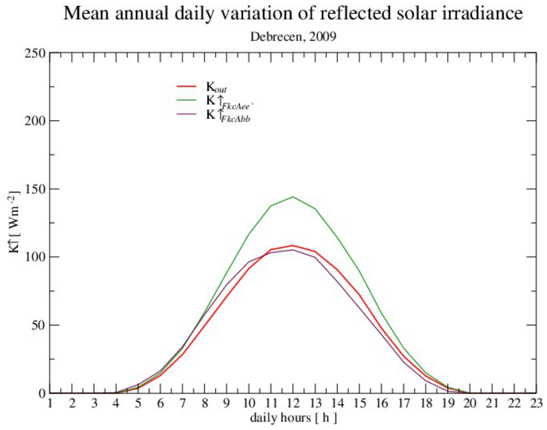
$K_{out}$	Reflected solar irradiance is part of global solar irradiance that is reflected from the Earth’s surface. It depends on the global solar irradiance and the surface albedo (function of the angle of solar elevation and characteristics of the ground surface).
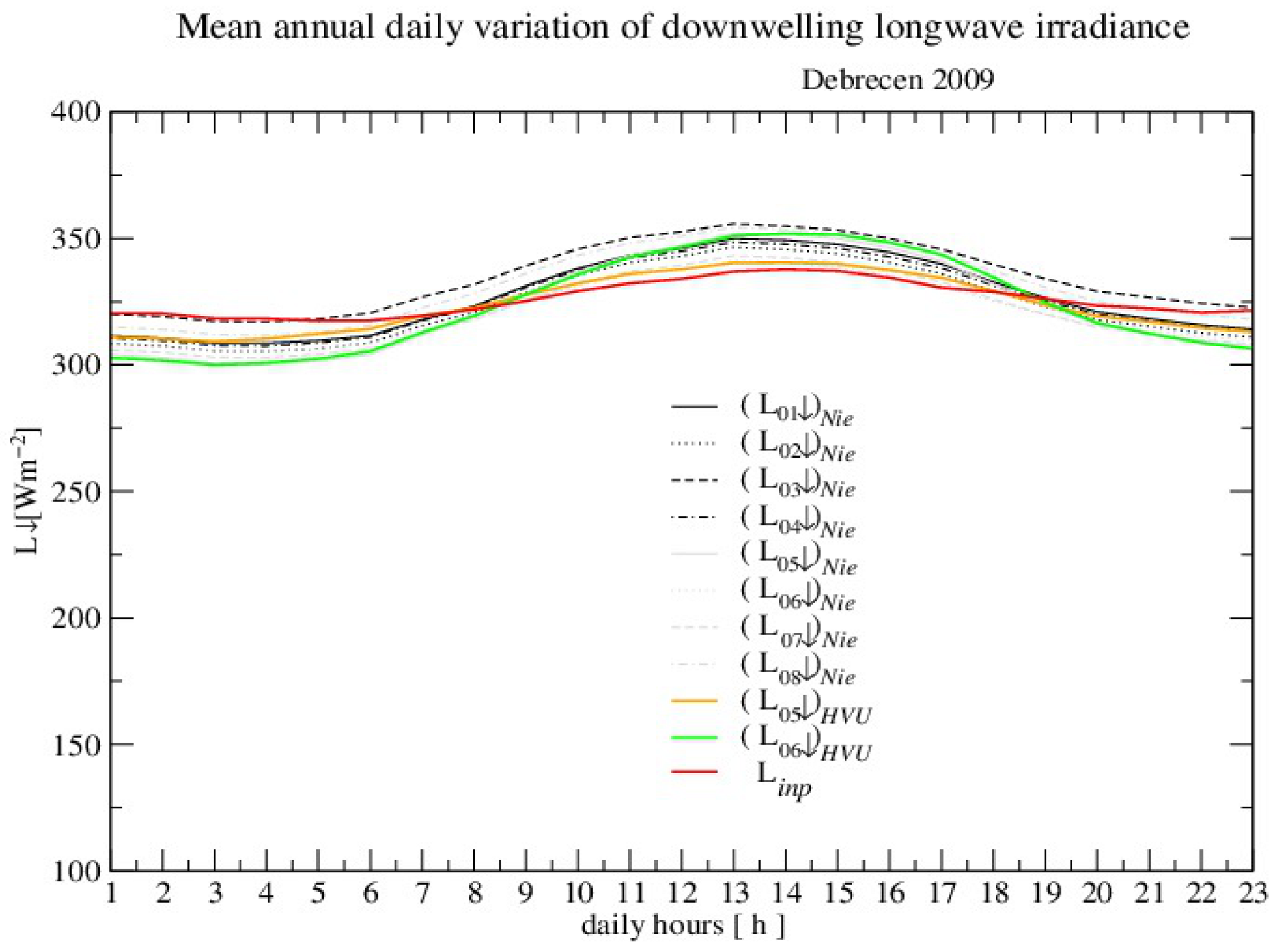
$L_{inp}$	Incoming longwave (LW) irradiance is a downward flux of thermal radiation emitted from the atmospheric molecules (such as H2O, CO2 and O3); aerosol particles and clouds per unit horizontal area in a given time period. It depends, first of all, on cloudiness, temperature precipitable water and turbidity of the atmosphere.
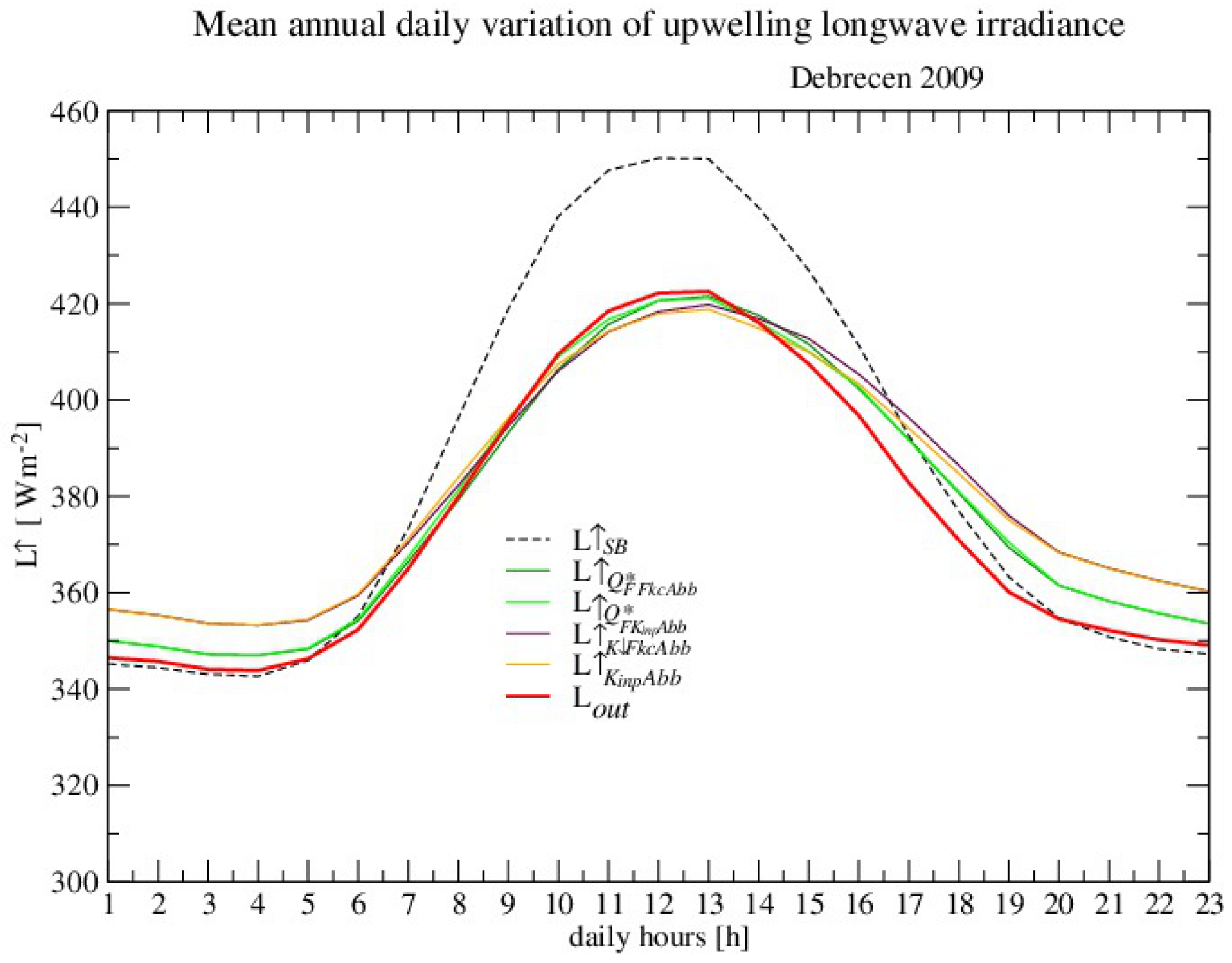
$L_{out}$	Outgoing (upwelling) longwave irradiance represents a redistribution of the absorbed global solar irradiance. The power of this energy emitted from the Earth’s surfaces per unit area and in the given time is called thermal (terrestrial) irradiance. Besides the global solar irradiance, it depends on the temperature of the Earth’s surface (or atmospheric temperature).
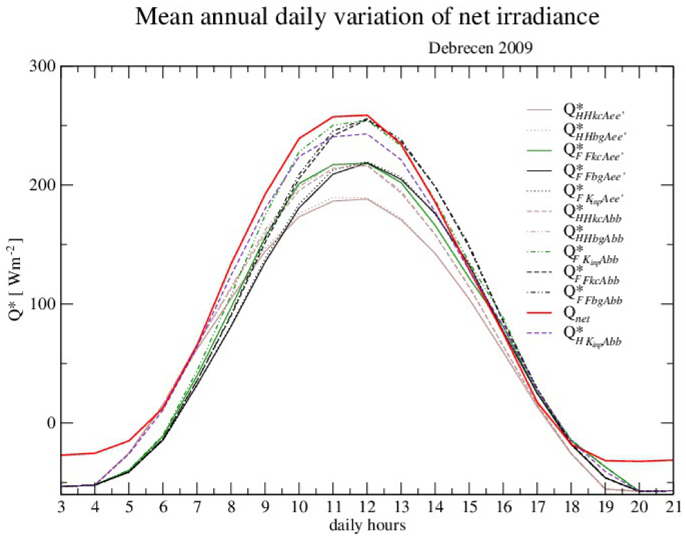
$Q_{net}$	Net irradiance is often convenient to split into four components: $K_{inp}$, $K_{out}$, $L_{inp}$ and $L_{out}.$ Therefore, net irradiance is a sum of these components. $$Q_{net}=K_{inp}-K_{out}+L_{inp}-L_{out}$$ (1) In our case, the signs of all the surface radiation balance components were positive or zero.

Net irradiance is necessary fuel for all motion processes in the atmosphere. Energy budget on the Earth surface in the case of the quasi-steady state of PBL, when there is no heating or cooling, sees the net irradiance as a sum of the sensible heat flux, $H$, latent heat flux, $LE,$ and flux into or from the ground, $Q_G$.

$$Q_{net}=H+LE+Q_G$$

(2)

Accordingly, $Q_{net}$ is key connection between radiation and stability of the atmosphere.

In order to estimate the upper irradiances, the next variables are measured or derived from routine SYNOP reports and the metadata about the location where measurements are conducted:

ϕ	The angle of solar elevation (rad)
φ	Latitude (rad)
λ	Longitude (rad)
h	Hour angle (rad)
$h_H$	Hour angle used in [5] (rad)
$h_F$	Hour angle used in [11] (rad)
t	Time UTC
DOY	Day of the year
$\mathsf{\Delta }{t}_d$	The duration of full rotation of the Earth (86,400 s)
$t_h$	The time distance from $t$ to the culmination of the Sun in seconds (s)
$t_{CET}$	Central European Time
EQT	Equation of Time, the difference between the true and averaged local times
N	Total cloud cover (octas)
$N_{CH}$	Covering of clouds genera cirrus, cirrocumulus and cirrostratus (octa)
$N_{CM}$	Covering of clouds genera altocumulus, altostratus and nimbostratus (octa)
$N_{CL}$	Covering of clouds genera stratocumulus, stratus, cumulus and Cb. (octa)
$A$	Albedo
$A_1$	Height solar elevation albedo for specific surface, according Geiger et al. [36]
${Aee}^{\prime }$	Calculated albedo depending on $A_{1 }$ and $\varphi ,$ according to Nyren and Gryning [37]
$Abb$	Calculated albedo depending on $N$ and $\varphi ,$ according to Beljaars and Bosveld [38]
${\epsilon }_0$	Surface emissivity
ρ	Air density (kg m−3); ρ = f (p, T, e)
$e$	Water vapor pressure (hPa)
$p$	Pressure (hPa)
$T$	Temperature (K)
$T_s$	Surface temperature (K)

2.3. Description of the Key Method

The measurement mentioned in Section 1 helps to better understand how solar energy changes the state of the atmosphere and how the state of the atmosphere influences the global solar irradiance and thermal irradiance on the Earth’s surface. There are some investigations that try to track the interaction between the Sun and Earth at some locations hourly through the relationship between: global solar irradiance, $K\downarrow$, reflected solar irradiance, $K\uparrow ,$ incoming longwave, LW, irradiance, $L\downarrow$, and outgoing LW irradiance, $L\uparrow$, in the surface and meteorological parameters. The methodologies that estimate the net radiation and all its components used in this paper are listed in

Table 1. List of applied parameterizations for radiation budget components. ($K\downarrow$, $K\uparrow$, $L\downarrow$, $L\uparrow$ and $Q^{\ast }$ are calculated, and $K_{inp} \mathrm{and} Q_{net }$ are the measured values.

Symbol	Radiation	Ref.	Abbr.	Eq.	Function of
$K_0\downarrow$	Global solar radiation for clear sky	[5]	$K_{0H}\downarrow$	(7)–(10) and (12)	= f ($\varphi$,$h_H, \phi , \lambda , t)$
		[11]	$K_{0F}\downarrow$	(7)–(9), (11) and (13)	= f ($\varphi$,$h_F,\phi ,\lambda ,t)$
$K\downarrow$	Global solar radiation	[5,39]	$K{\downarrow }_{Hkc}$	(12) and (14)	= f ($\varphi$,$h_H,\phi ,\lambda ,t, N)$
		[11,39]	$K{\downarrow }_{Fkc}$	(13) and (14)	= f ($\varphi$,$h_F,\phi ,\lambda ,t, N)$
		[5,40]	$K{\downarrow }_{Hbg}$	(12) and (15)	= f ($\varphi$,$h_H,\phi ,\lambda ,t,$$N_{CH},N_{CM},N_{CL})$
		[11,40]	$K{\downarrow }_{Fbg}$	(13) and (15)	= f ($\varphi$,$h_F,\phi ,\lambda ,t,$$N_{CH},N_{CM},N_{CL})$
$K\uparrow$	Reflected solar radiation	[36,37]	$K{\uparrow }_{FkcAee’}$	(16)	= f ($K\downarrow$,$A \left(\varphi ,A_1\right)$)
		[36,41]	$K{\uparrow }_{FkcAee’}$	(17)	= f ($K\downarrow$,$A \left(\varphi ,A_1\right)$)
		[36,38]	$K{\uparrow }_{FkcAbb}$	(20) Without snow	= f ($K\downarrow$,$A\left(\varphi ,A_1,N\right))$
		[36,38]	$K{\uparrow }_{FkcAbb}$	(21) With snow	= f ($K\downarrow$,$A\left(\varphi ,A_1,N\right))$
$L_0\downarrow$	Incoming LW radiation for Clear sky	[42,43]	$L_{01}\downarrow$	Table 11 row (1)	= f (T, e)
		[44]	$L_{02}\downarrow$	Table 11 (2)	= f (T, e)
		[45]	$L_{03}\downarrow$	Table 11 (3)	= f (T)
		[46]	$L_{04}\downarrow$	Table 11 (4)	= f (T, e)
		[47]	$L_{05}\downarrow$	Table 11 (5)	= f (T)
		[48]	$L_{06}\downarrow$	Table 11 (6)	= f (T, e)
		[43]	$L_{07}\downarrow$	Table 11 (7)	= f (T, e)
		[46]	$L_{08}\downarrow$	Table 11 (8)	= f (T, e)
$L\downarrow$	Incoming	[43,49]	${\left(L_{0i}\downarrow \right)}_{Jac}$	(36)	= f (N,$L_{0i,i=1,\dots ,8}\downarrow$)
	LW	[43,50]	${\left(L_{0i}\downarrow \right)}_{M\&C}$	(37)	= f (N,$L_{0i,i=1,\dots ,8}\downarrow$)
	radiation	[51]	${\left(L_{0i}\downarrow \right)}_{Izi}$	(38)	f (N,$L_{0i,i=1,\dots ,8}\downarrow$)
		[5,47]	${\left(L_{05}\downarrow \right)}_{HVU}$	(39)	= f (N,$L_{05}\downarrow$)
		[5,48]	${\left(L_{06}\downarrow \right)}_{HVU}$	(40)	= f (N,$L_{06}\downarrow$)
		[43]	${\left(L_{0i}\downarrow \right)}_{Nie}$	(41)	f (N,$L_{0i,i=1,\dots ,8}\downarrow ,L\uparrow$)
$L\uparrow$	Outgoing	SB low	$L{\uparrow }_{SBb}$	(30)	= f (${\epsilon }_0, T_s$)
	LW	[5,52,53]	$L{\uparrow }_{KFkcAbb}$	(31) and (33)	= f (T, $K{\downarrow }_{Fkc}$,$Abb)$
	radiation	[5,52,53]	$L{\uparrow }_{K_{inp}Abb}$	(31) and (33)	= f ($T, K_{inp},Abb)$
		[5,52]	$L{\uparrow }_{Q_F^{\ast }FkcAbb}$	(31) and (34)	= f (T,$Q_{F FkcAbb}^{\ast })$
		[5,52]	$L{\uparrow }_{Qnet}$	(31) and (34)	= f (T,$Q_{net}$)
$Q^{\ast }$	Net radiation	[5]	$Q_{H HkcAe{e}^{\prime }}^{\ast }$	(22)	= f ($K{\downarrow }_{Hkc}, {Aee}^{\prime }, T,N)$
	$Q_H^{\ast }$	[5]	$Q_{H HkcAbb}^{\ast }$	(22)	= f ($K{\downarrow }_{Hkc}, Abb, T,N)$
		[5]	$Q_{H HbgAe{e}^{\prime }}^{\ast }$	(22)	= f ($K{\downarrow }_{Hbg}, {Aee}^{\prime }, T, N)$
		[5]	$Q_{H HbgAbb}^{\ast }$	(22)	= f ($K{\downarrow }_{Hbg}$,$Abb, T, N)$
		[5]	$Q_{H K_{inp}Ae{e}^{\prime }}^{\ast }$	(22)	= f ($K_{inp}$, ${Aee}^{\prime }, T,N)$
		[5]	$Q_{H K_{inp}Abb}^{\ast }$	(22)	= f ($K_{inp}$, $Abb, T,N)$
	Net radiation	[11]	$Q_{F FkcAe{e}^{\prime }}^{\ast }$	(23)	= f ($K{\downarrow }_{Fkc}, {Aee}^{\prime }, T,N)$
	$Q_F^{\ast }$	[11]	$Q_{F FkcAbb}^{\ast }$	(23)	= f ($K{\downarrow }_{Fkc}$, $Abb, T,N)$
		[11]	$Q_{F FbgAe{e}^{\prime }}^{\ast }$	(23)	= f ($K{\downarrow }_{Fbg}$, ${Aee}^{\prime }, T,N)$
		[11]	$Q_{F FbgAbb}^{\ast }$	(23)	= f ($K{\downarrow }_{Fbg}$, $Abb, T,N)$
		[11]	$Q_{F K_{inp}Ae{e}^{\prime }}^{\ast }$	(23)	= f ($K_{inp}$, ${Aee}^{\prime },\rho )$
		[11]	$Q_{F K_{inp}Abb}^{\ast }$	(23)	= f ($K_{inp}$, $Abb,\rho )$

below. Each methodology is represented through its source, i.e., reference (ref.), abbreviation (abbr.) and equations number (eq.), which describe the components of irradiance as a function of variables written in parentheses in the last column.

List of lower indices in Table 1:

${}_H$	Holstlag and Van Ulden methodology for $K_0\downarrow$ calculation [5]
${}_F$	Foken methodology for $K_0\downarrow$ calculation [11]
${}_{kc}$	Kasten and Czeplak [39] parameterization of cloudiness for incoming solar radiation
${}_{bg}$	Burridge and Gadd [40] parameterization of cloudiness for incoming solar radiation
${}_{SBb}$	Stefan–Boltzmann (SB) low with ${\epsilon }_0=1$
${}_{SBg}$	Stefan–Boltzmann low with ${\epsilon }_0=0.98$
${}_{Jac}$	Cloudiness parameterization for downwelling LW radiation based on Jacobs [49]
${}_{M\&C}$	Cloudiness parameterization for downwelling LW radiation based on Maykut and Church [50]
${}_{M\&C}$	Cloudiness parameterization for downwelling LW radiation based on Iziomon et al. [51]
${}_{Izi}$	Cloudiness parameterization for downwelling LW radiation based on Iziomon et al. [51]
${}_{HVU}$	Cloudiness parameterization for downwelling LW radiation based on Swinbank [47] and Dilley and O’Brien [48]
${}_{Nie}$	Cloudiness parameterization for downwelling LW radiation based on Niemelä et al. [43]

Each an estimated radiation component is compared with the measurements and discussed through statistical errors: BIAS, MAE, RMSE and correlation coefficient ($r$). Statistical errors for the estimated $X_{\mathrm{est}}$ and measured $X_{\mathrm{meas}}$ values are calculated by:

$$\mathrm{BIAS}=\frac{1}{n}·{\displaystyle \sum }_{i=1}^n\left[{\left(X_{\mathrm{est}}\right)}_i-{\left(X_{\mathrm{meas}}\right)}_i\right]$$

(3)

$$\mathrm{MAE}=\frac{1}{n}·{\displaystyle \sum }_{i=1}^n\left|{\left(X_{\mathrm{est}}\right)}_i-{\left(X_{\mathrm{meas}}\right)}_i\right|$$

(4)

$$\mathrm{RMSE}=\sqrt{\frac{1}{n-1}·{\displaystyle \sum }_{i=1}^n{\left[{\left(X_{\mathrm{est}}\right)}_i-{\left(X_{\mathrm{meas}}\right)}_i\right]}^2}$$

(5)

$$r=\frac{\frac{1}{n-1}·{{\displaystyle \sum }}_{i=1}^n\left\{\left[{\left(X_{\mathrm{est}}\right)}_i-{\overline{X}}_{\mathrm{est}}\right]·\left[{\left(X_{\mathrm{meas}}\right)}_i-{\overline{X}}_{\mathrm{meas}}\right]\right\}}{\sqrt{\frac{1}{n-1}·{{\displaystyle \sum }}_{i=1}^n\left\{{\left[{\left(X_{\mathrm{est}}\right)}_i-{\overline{X}}_{\mathrm{est}}\right]}^2·{\left[{\left(X_{\mathrm{meas}}\right)}_i-{\overline{X}}_{\mathrm{meas}}\right]}^2\right\}}}$$

(6)

where ${\overline{X}}_{\mathrm{est}}$ and ${\overline{X}}_{\mathrm{meas}}$ are the mean values of the modeled and measured hourly values, respectively, and n is the number of cases (measured hours).

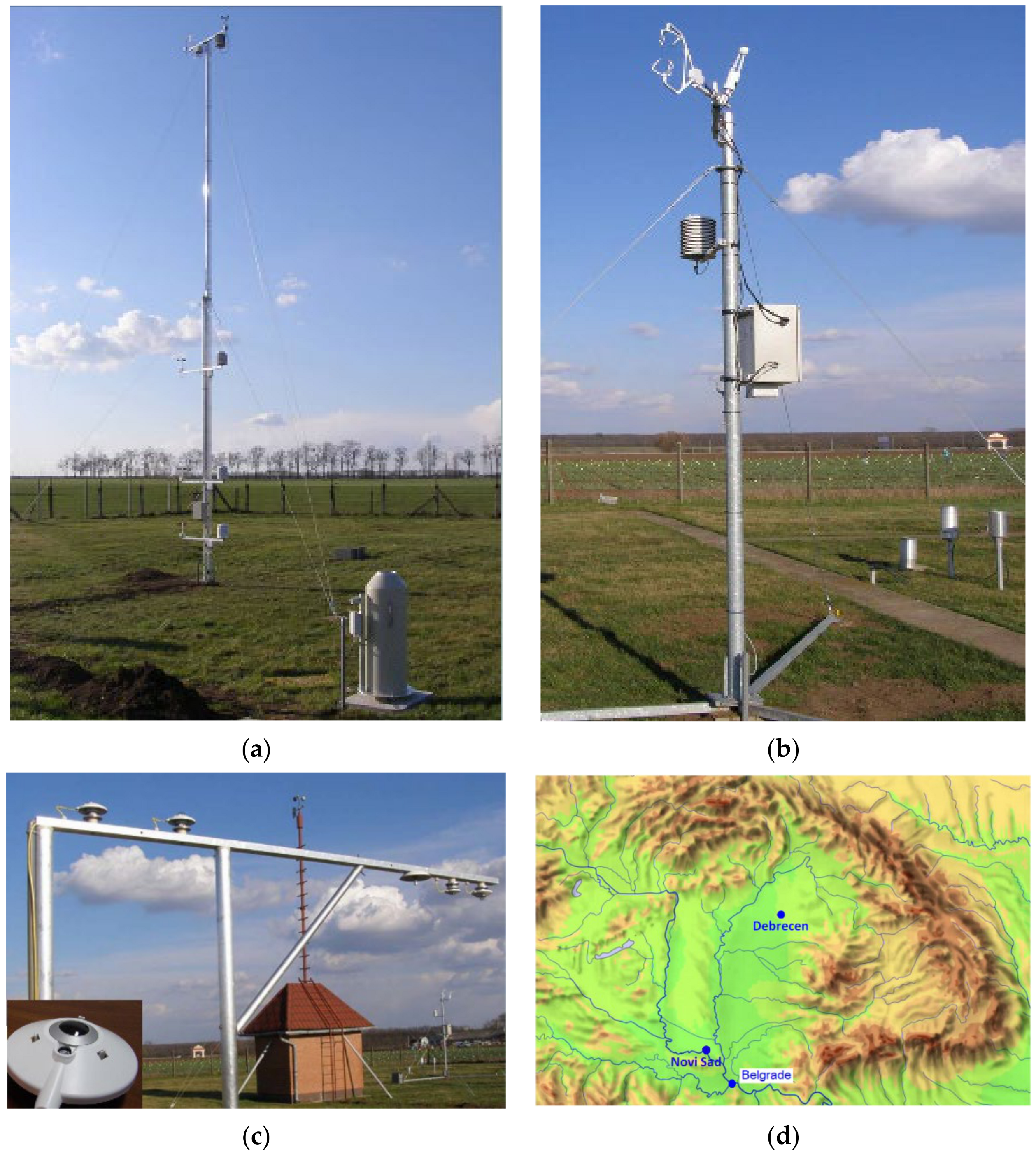
3. The Description of the Datasets

The Agrometeorological Observatory in Debrecen is on a flat, mostly homogenous terrain in agricultural surroundings with geographic coordinates: $\phi =47.5291°$ (latitude) and $\lambda =21.6397°$ (longitude).

There is a meteorological 10-m mast with profile measurements of ten-minute average values of:

• temperature, relative humidity and wind speed, at 1, 2, 4 and 10 m;
• infrared ground surface temperature;
• two levels of soil temperature and humidity (5 and 10 cm) and
• all radiation balance components: global solar radiation or $K_{inp}$, reflected solar radiation $K_{out}$, incoming longwave (LW) radiation $L_{inp}$ and outgoing LW radiation $L_{out}$.

Together with the station’s pressure, precipitation and snow cover obtained from routine meteorological measurements and observations, we used a 2-m temperature and relative humidity and 10-m wind speed from the mast. The momentum, CO₂ and sensible and latent heat fluxes were also measured directly using the CSAT-3 and LI-7500 instruments with the Campbell data acquisition program.

Standard meteorological measurements, including cloudiness and visibility, were provided from the SYNOP station in Debrecen Airport (12882) 8.5 km from the Agrometeorological Observatory [54,55].

The new generation of micrometeorological measurements started in 2008. The instruments were initially factory-calibrated, and a year-long dataset was investigated in the year 2009. That is why the first full year has been chosen for model development. For the long-term comparative study of the developed calculation methods, two test periods were selected. The first was 3 years between 2008 and 2010 when cloud and present weather observations were made hourly at Debrecen Airport (SYNOP station No. 12882). The second, longer test period was 7 years between 2011 and 2017. Namely, after that, from 2011, only partial cloud observations took place at night, so we checked the parameterization of the shortwave radiation balance components and, on occasion, the longwave radiation balance components. The entity responsible for the operation of Agrometeorological Observatory Debrecen was changed in 2017. Data with quality control has been available to us until this year. Since 2018, the measuring site has been operating as a “backup” site with limited data access because there has been a new measuring site installed.

Long-term agroclimatological investigations and reorganization of the high-precision radiation and micrometeorological measurements are in progress at Agrometeorological Observatory Debrecen. The location of the observation in the Pannonian Basin, main measurement items and the instrumentation are presented in Figure 1 and

Table 2. Instrumentation used on the micrometeorological measurements in Agrometeorological Observatory Debrecen (Figure 1) from 2008.

No	Instrument	Height	Variables	Comment
Eddy covariance measurements
1	Campbell Scientific CSAT3	4 m	Wind speed components ($u, v, w$) (m/s), sound speed ($c$) (m/s), sonic temperature ($T_{sonic}$) (K)	10 Hz time resolution
2.	LI-7500	4 m	Open path H2O/CO2 sensor (H2O concentration) (ppt) (CO2 concentration) (ppm) pressure ($p$) (hPa)	10 Hz time resolution
3	Campbell Scientific CR1000	1.6 m	Collecting and calculating of Eddy covariance fluxes	10 Hz sampling frequency and 30 min time period for flux calculations.
Profile measurements
4	Vaisala WAA151	10, 4, 2, 1 m	Wind speed ($U$) (mean, max, std.) (m/s)	Cup anemometer
5.	Vaisala HMP155	10, 4, 2, 1 m	Temperature ($T$) (°C) and relative humidity (Rh) (%)	With Vaisala DTR13 shield
Surface radiation balance components
6	Kipp&Zonen CMP11 pyranometer	2 m	Shortwave downward (downwelling) radiation (W m−2)
7	Kipp&Zonen CMP6 pyranometer	2 m	Shortwave upward (upwelling) radiation (W m−2)
8	Kipp&Zonen CGR4 pyrgeometer	2 m	Longwave downward (downwelling) radiation (W m−2)
9	Kipp&Zonen CGR3 pyrgeometer	2 m	Longwave upward (upwelling) radiation (W m−2)
10	Apogee IRTS-P	2 m	Soil surface temperature
Soil measurements
11	Campbell Scientific TCAV	−0.04 m	Soil temperature (°C)
12	Campbell Scientific CS616	−0.04 m	Soil water content (%V)
13	Hukseflux HFP01SC	−0.08 m	Soil heat flux plats (2) (W m−2)
Other
14	PG200 weigting gauge	1 m	precipitation (mm)
15	Campbell Scientific CR1000	1.6 m	Collecting sensors output of profile, radiation budget components, surface, soil and precipitation measurements.	0.5-Hz sampling frequency and 10 min averaging

.

The measurement of solar radiation balance components is part of the measuring program of the surface observing system of the Hungarian Meteorological Service. The operation of observing the system and calibration of sensors is regulated by the ISO9001:2015 quality control system. The calibration of solar radiation sensors is done according to the relevant working instructions; therefore, the calibration of the solar radiation sensors of Agrometeorological Observatory Debrecen is done the same way. Regarding the shortwave sensors, the reference instrument is an HF-type absolute cavity pyrheliometer (s.n. 19746) that has been calibrated at International Pyrheliometer Comparisons (IPC-s) at the World Radiation Centre (WRC) in Davos every five years since 1980. In the case of longwave sensors, the reference sensors are an Eppley PIR (s.n. 29582F3) that was calibrated two times at WRC Davos between 2006 and 2014 and a Kipp&Zonen CGR4 (s.n. 080066) that was calibrated during IPC-XII in 2015. The calibration of the radiation sensors was done with parallel measurements between reference and site instruments, which happened in every two years between 2008 and 2013 and every three years after 2013. The history of the calibrations shows that, in the case of shortwave down- and upward sensors, the averaged differences among the values of reference and site instruments did not exceed ±1.5% and ±1%, respectively, if the level of irradiance was over 200 W m⁻². Regarding the downward and upward longwave sensors, the differences, because the downward sensor was not shaded and ventilated, were between ±3.5% and 2%, respectively. The addition of the personal checking of measuring sites was done every 3 months when the leveling of the sensors was checked and cleaning was done. The detailed calculations of uncertainty of the calibration factors of the solar sensors is not part of the relevant working instructions.

4. Assessments of Solar Irradiance

The Earth’s surface, the basic energy transfer area for atmospheric processes, is heated by the absorption of Sun shortwave radiation, $K\downarrow$. A small part of this radiation, depending on the complexity of the surface, the state of the ground surface, the Sun’s position on the sky, visibility and cloudiness, is reflected back to the sky, $K\uparrow$.

The mean annual daily variation of calculated $K\downarrow$ and $K\uparrow$, as well as measured $K_{inp}$ and $K_{out}$ irradiance, for the clear and cloudy sky are represented by taking the different procedures for their calculations. The statistical errors (See Section 2.3) of their calculations represent the reliability of these calculations.

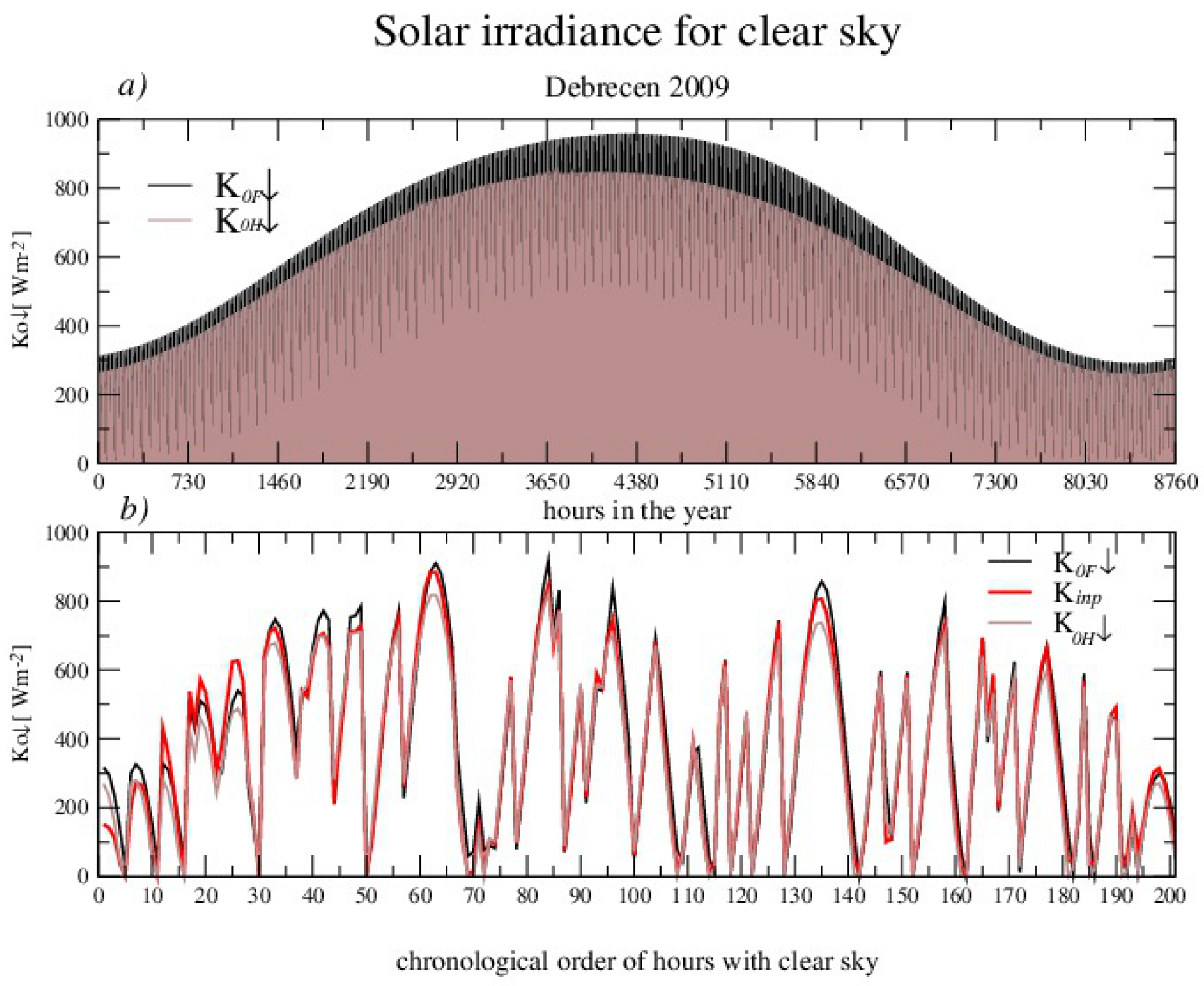
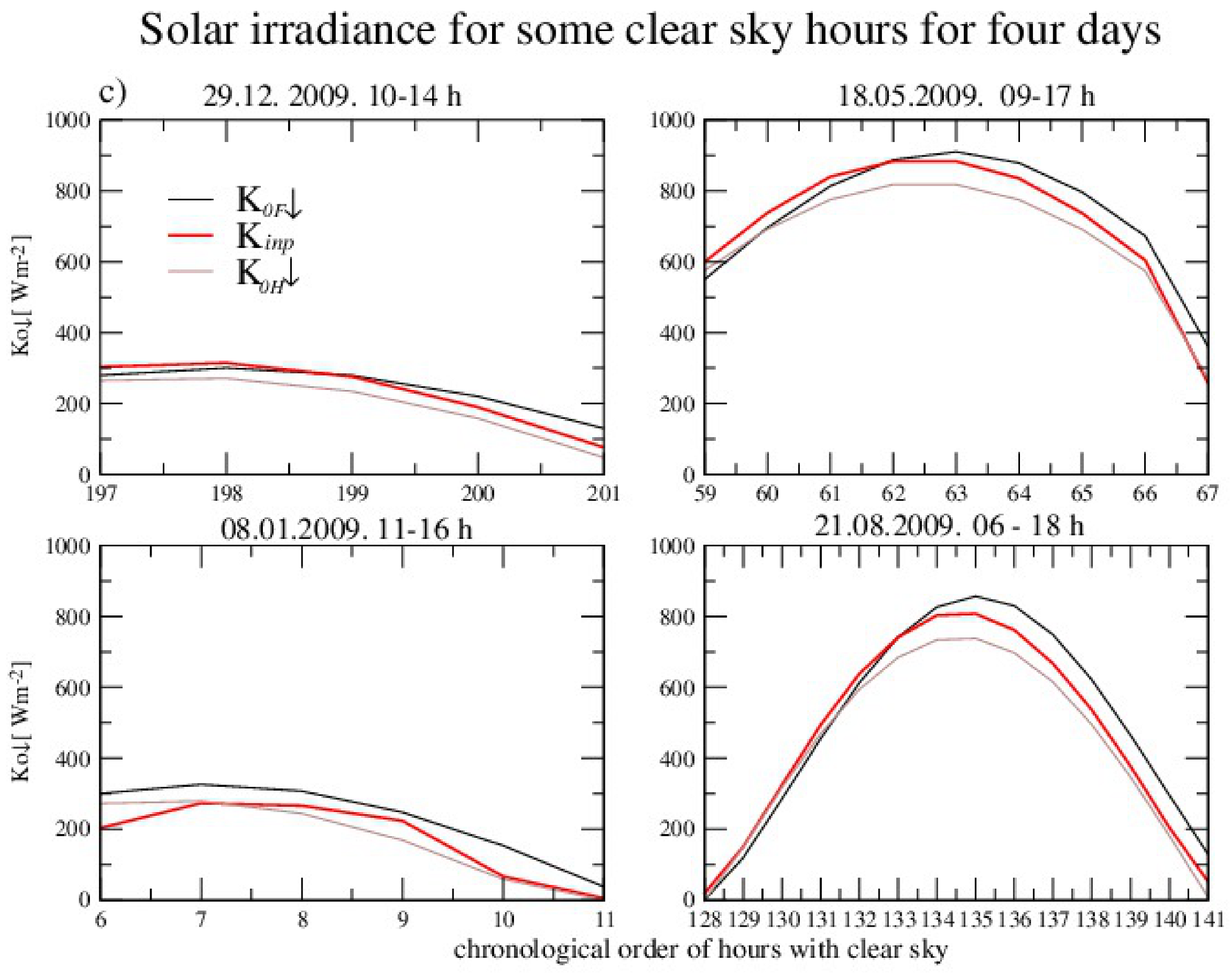
4.1. Assessments of Downwelling Shortwave Solar Radiation for Clear Sky

The astronomical quantities and downwelling solar radiation are calculated using Foken [11] and Holtslag and Van Ulden [5] methodology. Both well-known methods estimate downwelling solar radiation as a function of $\varphi$, the angle of solar elevation. This angle is a function of: solar declination, $\delta$, latitude, $\phi$, and hour angle, $h$ (all angles are in radians):

$$\sin \varphi =\sin \delta ·\sin \phi +\cos \delta ·\cos \phi ·\cos h$$

(7)

$$\delta =\arcsin \left(0.398·\sin {\phi }_s\right)$$

(8)

where ${\phi }_s$, the solar latitude, is

$${\phi }_s=4.871+0.0175·DOY+0.033·\sin \left(0.0175·DOY\right)$$

(9)

and $DOY$ is the Day of the year.

Holtslag and Van Ulden [5] used the hour angle as a function of $\lambda$, east longitude in radians and time $t$ as UTC time. The equation of hour angle, $h_H,$ is calculated as follows:

$$h_H=\lambda +0.043·\delta -0.033·\sin \left(0.0175·DOY\right)+\pi \left(t/12\right)-\pi$$

(10)

Foken [11] took the hour angle, $h_F,$ as a function of $\mathsf{\Delta }{t}_d$, the duration of full rotation of the Earth (between two midnights = 86,400 s), and $t_h$, the time distance from $t$ to culmination of the Sun in seconds.

$$h_F=2\pi ·\left(t_h/\mathsf{\Delta }{t}_d\right)$$

(11)

where $t_h=t_{CET}-\left[12+EQT+\left(15-\lambda \right)·\frac{4}{60}\right] \mathrm{and} EQT={\displaystyle \sum }_{n=0}^{12}{x}_n·DO{Y}^n$, where the longitude, $\lambda$, here is in degrees ($°$), $EQT$ is the difference between the true and averaged local time and $t_{CET}$ is the Central European Time. From tables of time equations [56] for 15° E and 50° N, Göckede [57] calculated an approximation equation for $EQT,$ and the coefficients $\left\{x_0, x_1, \dots , x_{12} \right\}$ were listed in Foken [11].

After checking the agreement between Equations (10) and (11), one notices that the resultant angles of solar elevation (see, also, Equation (7)) are very similar but not same. They have a maximum at the same hour but, obviosly, not at the same moment. At the hour with maximum solar elevation, the Foken’s value of the solar elevation angle is about 0.6° greater than Holstlag’s during the day of the sumer solsticium and about 0.2° greater than Holstlag’s during the winter solsticium. Concerning the daily circling, it looked that Foken’s solar elevation lasted about 20–25 min after Holstlag’s. This deviation was established arbitrary based on Figure 2a, on which the x-axis represents “hours in the year” and y-axis represents solar elevation. This deviation was not the same every day, and 20–25 min was the annual maximum. It happened on August 2, when the differences between the angles of solar elevation were a little smaller than 6.5°. In 285 out of 8760 h, these differences were greater than 6°; in 1104 h, they were greater than 5° and, in 4145, they were greater than 3°.

Using the angle of solar elevation $\varphi$, which is calculated with the hour angle described by Equations (10) and (11), downwelling the clear sky solar radiation $K_0\downarrow$ following Holstlag’s calculations based on reference [5] is:

$$K_{0H}\downarrow =a_{1}sin\varphi +a_2$$

(12)

Constants $a_1$ and $a_2$ are determined by the least squares method from measurements of global solar irradiance for the clear sky and $\varphi \ge 23°$. Based on the test calculations in Budapest (12,843), they are $a_1=990$ and $a_2=-30$.

Another methodology was Foken’s calculation of the downwelling solar radiation for clear sky situations based on references [1,11]]:

$$K_{0F}\downarrow =S·{\left(\frac{r_0}{r}\right)}^2·\sin \varphi ·\left(0.6+0.2·\sin \varphi \right)$$

(13)

where $r_0$ and $r$ are the mean and actual distances from the Earth to the Sun. The ratio of both can be determined according to Hartmann (1994) (see reference [11]) as a sum of the first three components of the Fourier series. The argument of the Fourier series is $2\pi DOY/265$ (denominator is 266 in the case of a leap year), and the coefficients of the Fourier series are listened in reference [11]. The angle of solar elevation is calculated with the hour angle described by Equation (11). $S$ is the solar constant ($S=1368 {\mathrm{W} \mathrm{m}}^{-2})$.

Although during the year 2009, there were only 201 h both with $\phi >0$ and with clear skies, based on the SYNOP station at the airport in Debrecen (12882) (Figure 2), statistical errors for this set of data have also been investigated (

Table 3. Statistical errors for clear sky irradiance based on Foken’s and Holtslag’s separately.

Statistical Error	BIAS	MAE	RMSE	Correlation $\mathbf{Coefficient} \left(\mathit{r}\right)$
$K_{0F}\downarrow$	+14.6 W m−2	40.7 W m−2	52.8 W m−2	0.97
$K_{0H}\downarrow$	−17.2 W m−2	32.1 W m−2	44.0 W m−2	0.97

.)

Based on the 201 clear sky hours, the Foken’s calculation made an error over 100 W m⁻² in 11-h data, while Holtslag’s calculation had nine such situations. The errors over 50 W m⁻² took up about one-quarter of the hourly data, mostly during the winter period, and were fewer for Holtslag’s than Foken’s calculations.

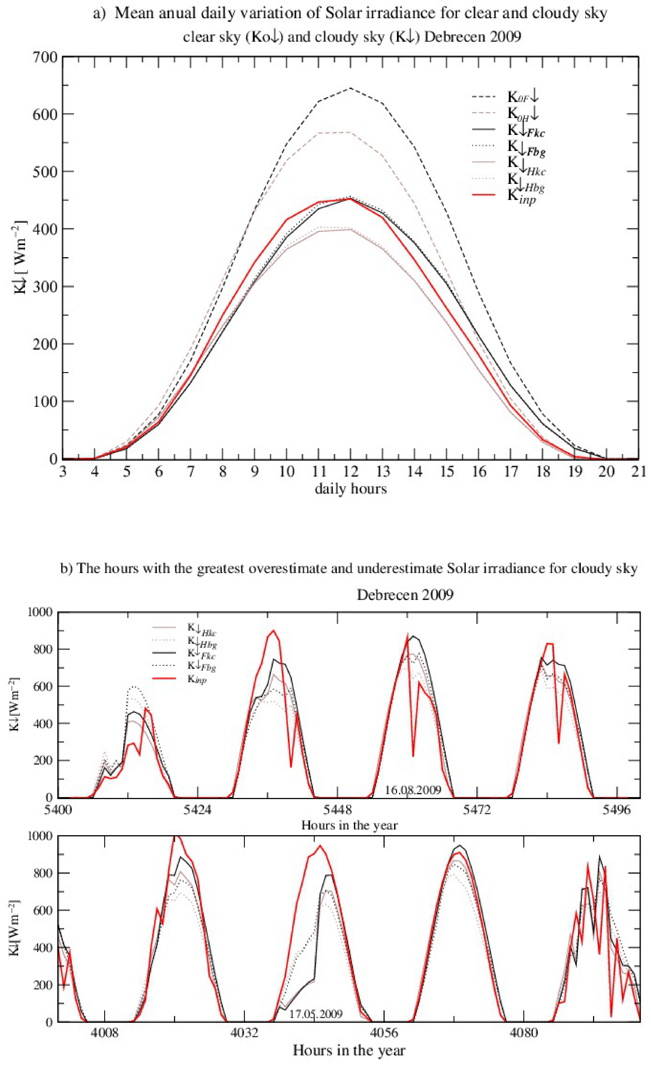
4.2. Assessments of Downwelling Shortwave Solar Irradiance for All Sky Condition

To include cloudiness in the calculation of shortwave incoming solar irradiance, we applied two widely used methodologies based on Kasten and Czeplak [39]:

$$K_{kc}\downarrow =K_0\downarrow \left[1-0.75·{(N/8)}^{3.4}\right]$$

(14)

and Burridge and Gadd [40]:

$$K_{bg}\downarrow =K_0\downarrow \left(1-0.4\frac{N_{CH}}{8}\right)\left(1-0.7\frac{N_{CM}}{8}\right)\left(1-0.4\frac{N_{CL}}{8}\right)$$

(15)

where $N$ is total cloud cover that goes from 0 for clear skies to 8 octa for total cloudy skies, and $N_{CH}$, $N_{CM}$ and $N_{CL}$ are cloud covers of high, middle or low clouds, respectively.

The first method was described by Holtslag and Van Ulden [5] and Nyren and Gryning [37]. This method was also popular in climatological investigations and applications requiring rough estimations of solar radiation on horizontal surfaces [58,59,60]. The second method was described by Stull [61] and used in different micrometeorological modeling works for radiation parameterization, such as in surface hydrological modelling or snow evolution system modeling [62,63]. The number of SYNOP stations with complex cloud observations, especially the cloudiness and cloud types, decreased with the installation of automatic surface weather stations from the mid-1990s [64]. Observations of cloud types are still generally performed by human observers and naturally have a few limitations [65]. Although it seems clear that the second method includes cloudiness in a more sophisticated way than the first, the lack of information about cloudiness for different levels: $N_{CH}$, $N_{CM}$ and $N_{CL}$, makes the first method more practical. Namely, in the case when the total cloud cover was 8 octa and the upper cloud levels were invisible, we had to approximate $N_{CM}$ and $N_{CH}$ and took $N_{CM}=N_{CH}=5$. Besides that, when $N=8$ and $N_{CL}<8$, we supposed that $N_{CM}=8$ or $N_{CH}=8$, which depended on the type of clouds. On the other hand, instead of a total cloud cover in the first method, effective cloudiness $N_{eff}=\left(N+N_{CL}\right)/2$ is used as an alternative solution in the calculation of $K_{kc}\downarrow$ whenever $N_{CL}$ is available from SYNOP.

Statistical errors for global solar irradiance for the four investigated models, comparing 4022 h during the year 2009, when all data necessary for the calculations was available ($K_{inp}>0 {\mathrm{W} \mathrm{m}}^{-2})$, are shown in

Table 4. Statistical errors for global solar irradiance by Holtslag’s (H) [5] and Foken’s (F) [11] clear sky irradiance calculations, together with both methods for including cloudiness using the Kasten and Czeplak (kc) [39] and Burridge and Gadd (bg) [40] methodologies.

Method	BIAS [W m−2]	MAE [W m−2]	RMSE [W m−2]	$\mathbf{Correlation} \mathbf{Coefficient} \left(\mathit{r}\right)$
$K{\downarrow }_{Fkc}$	+5	71	109	0.90
$K{\downarrow }_{Fbg}$	+8	74	108	0.91
$K{\downarrow }_{Hkc}$	−12	69	109	0.91
$K{\downarrow }_{Hbg}$	−10	77	111	0.91 (0.85, 0.80)

. The errors were absolutely the same using either total or effective cloud cover.

About 3000 of 4022 h of data had absolute errors in estimation fewer than 100 W m⁻², but about 500 of them had errors greater than 200 W m⁻². There is no comment here whether these errors were the result of the crude method for estimation of the input solar irradiance or even sporadic errors in the measurements. Namely, the radiation balance components are measured with first-class radiation sensors separately using the Campbell CR1000 datalogger, so the measurements are quality-controlled and mostly reliable. Therefore, without analyzing the reason, all situations when the differences between the measured and estimated solar radiations were fewer than: 50, 100, 200,..., 700 W m⁻² were countered, and the results are shown in

Table 5. The total number of situations with absolute errors (AE) fewer than 50, 100,…, 700 W m⁻².

AE (W m−2)	<50	<100	<200	<300	<400	<500	<600	<700
$K{\downarrow }_{Fkc}$	2214	3174	3703	3914	3982	4009	4018	4022
$K{\downarrow }_{Fbg}$	2014	3022	3697	3920	4000	4019	4022	4022
$K{\downarrow }_{Hkc}$	2455	3207	3720	3916	3983	4011	4019	4022
$K{\downarrow }_{Hbg}$	2140	2988	3668	3931	4008	4022	4022	4022

.

After this counting, we recalculated statistical errors for 3500 h of data when all the methods had absolute errors fewer than 200 W m⁻². In that case, the MAE became smaller around 25% and RMSE around 50%, and the coefficient of correlation grew to 0.96, while the BIAS stayed similar. The few greatest absolute errors (>200 W m⁻²) seemed to be connect to the Kasten and Czeplak [39] method for describing cloudiness, because after excluding these situations, the RMSE and MAE became 10% smaller for this method than for the Burridge and Gadd [40]-type cloudiness parameterizations for both clear sky calculations.

Relative errors were fewer than 10% for only 18–25% of the hourly data. Both methods look very similar through statistical errors (Table 4). Looking at the absolute errors, one notices that the Kasten and Czeplak [39] cloud parameterization has a greater number of hours with errors smaller than 50 W m⁻², although the few greatest AE relate to this parameterization. All methods have relative errors below 25% in about 45% of data hours. The usual errors are connected with the short periods when the sky fast becomes either overcast or clear, or when solar elevation is low, especially during the winter period.

Although it is not very obvious which clear sky model and model for cloudiness is better (Figure 3 and Table 4 and Table 5), we clearly notice that:

(1)

Foken’s clear sky model, together with Kasten and Czeplak [39] methodology, were the best during unstable stratification when the solar elevation was high, although a few of the greatest absolute errors happened then (Figure 3b).

(2)

Holtslag’s clear sky model and Burridge and Gadd [40] cloudiness parameterization were the best for low solar elevation, when, especially during sunset, Foken’s calculation permanently overestimated the measurements.

One can conclude that both clear sky methods and both cloudiness methods are very useful tools for data quality control through intercomparison tests that check the relationship between cloudiness and global solar radiation at midday and separately at sunset or sunrise.

4.3. Assessments of Upwelling Shortwave Solar Irradiance

The upwelling solar radiation is part of downwelling solar radiation, which is reflected from the Earth’s surface and the atmosphere. The ratio of reflected to incoming shortwave radiation is called albedo. It depends on the angle of solar elevation, cloudiness and composition and state of the Earth’s surface. It is not measured on a routine basis. There are hourly values of the albedo as the fraction of the measured incoming shortwave radiation that is reflected in a Debrecen dataset.

Assessments of Albedo

In 1995, Geiger et al. [36] offered a classification where high solar elevation albedo depended on the surface type and varied from 0.024 for rough seas to 0.98 for clean snow. Since there was no data in Debrecen for “state of the ground with/without snow or measurable ice cover”—WMO SYNOP code tables 0901 E and 0975 E’, the hourly data about precipitation and present and past weather, as well as the temperature, must be used in order to classify the “state of the ground”. Namely, the nearest stations that included the “state of the ground” in the SYNOP reports at 06 UTC were: the station WMO 13174 Kikinda (in Serbia) and WMO 11968 Kosice (in Slovakia). In this paper, the albedo A was calculated for three different values of $A_1 :$ $A_1=0.11$ for wet soil (precipitation in present or past weather), $A_1=0.25$ for dry soil (nice weather) and $A_1=0.85$ for snow (snow cover).

The equation that was adopted after reference [66] and used by Nyren and Gryning [37] expresses albedo, $A$, as a function of the solar elevation angle (in degrees):

$${Aee}^{\prime }=A_1+\left(1-A_1\right)·\exp \left(0.1·\left(90-\varphi \right)\right)$$

(16)

The other similar empirical equation was used by references [67,68]. This type of methodology for the calculation of albedo that depends on the solar elevation and the soil wetness has been applied up to the present day [41].

$${Aee}^{\prime }=A_1+\left(1-A_1\right)·\exp (-0.1\varphi -\left(1-A_1\right)/2)$$

(17)

Statistical errors for proposal albedos are the same for the first three decimal places, using both Equations (16) and (17). Due to that, only one set of results is presented. The calculated albedo compared with the measurements is illustrated in

Table 6. Statistical errors: BIAS, MAE and RMSE based on the Nyren and Gryning [37] model of albedo for all data and separately for nice weather without snow cover ($A_1=0.25$), for weather with snow cover and without precipitation ($A_1=0.85$) and, finally, for precipitation weather ($A_1=0.11$).

Statistical Error for Albedo Aee’ Data Type	BIAS	MAE	RMSE	Correlation $\mathbf{Coefficient} \left(\mathit{r}\right)$
All data	0.055	0.076	0.118	0.08
Nice weather $A_1=0.25$	0.046	0.064	0.078	−0.19
Snow caver $A_1=0.85$	0.150	0.179	0.269	−0.16
Precipitation $A_1=0.11$	−0.072	0.076	0.179	<0.10

.

Without hours with precipitations and snow cover, a total of 3473 out of 4022, the statistical errors were smaller, while the 126 h with precipitation and 423 with snow cover without precipitation had expectedly greater errors.

Besides this calculation, we tried to find albedo as a function of solar elevation in Debrecen in a similar way as Duynkerke [69], as well as Beljaars and Bosveld [38]. They suggest that albedo depends on the angle of solar elevation and on the relation between diffuse and total incoming solar radiation, i.e., cloud cover.

Following their idea about the dependences of the albedo of the cloud cover, firstly, a linear function $A=A\left(\varphi \right)$ for clear skies is calculated, using observations of albedo and Foken’s calculation for solar elevation during clear sky conditions ($N=0$). For the 178 h without snow cover, this linear dependency is:

$$A=0.33-0.19·\sin \varphi$$

(18)

$$A=0.83-0.14·\sin \varphi$$

(19)

Following idea described in reference [38] alongside this equation, cloudiness is included to describe albedo in nonclear sky conditions using the least squares method for the different forms of the functions without and with snow cover surface. Beljaars and Bosveld [38] introduced the relation of downwelling diffuse incoming solar radiation, $SRDd$, and totally downwelling solar radiation, $SRd$, as a factor with leading influence on the albedo. Since there is no solar radiation instrument equipped with a shadow band at Agrometeorological Observatory Debrecen, taking that diffuse radiation as 10% of the total downward solar radiation for clear skies ($N=0$) and 100% for cloudy skies ($N=8$), we supposed that their ratio rises linearly between 0.1 and 1.0 with the rising cloudiness. Therefore, it used $\left(0.125·N-0.1\right), \mathrm{instead} \mathrm{of} \left(SRDd/SRd-0.1\right)$, given by reference [38]. For 3473 situations without snow cover and precipitation, when $N\ge 0$, we obtained:

$$Abb=0.33-0.19·\sin \varphi -\left(0.125·N-0.1\right)·\left(0.33-0.49·\sin \varphi \right)$$

(20)

For 423 data with snow cover, we obtained:

$$Abb=0.83-0.14·\sin \varphi -\left(0.125·N-0.1\right)·\left(0.14-0.14·\sin \varphi \right)$$

(21)

For hourly data both with precipitation and snow, we took $A=0.2$.

The statistical errors obtained from these calculations were significantly smaller than in previous calculations, except in the case of precipitation (

Table 7. Same as Table 6 but for the Beljaars and Bosveld [38] method for the estimation of albedo.

Statistical Error for Albedo Abb Data Type	BIAS	MAE	RMSE	Correlation $\mathbf{Coefficient} \left(\mathit{r}\right)$
All data	−0.023	0.069	0.118	0.79
Nice weather    $A_1=0.25$	−0.024	0.053	0.085	0.22
Snow caver    $A_1=0.85$	0.011	0.117	0.221	0.15
Precioitation    $A_1=0.11$	0.108	0.168	0.287	<0.10

). Useful, statistical significance correlation was formed in the case of all data ($r=0.79),$ but in all three independent cases, the absolute values of the correlation coefficients were below 0.3, so there were no useful connections for the practices among the measured and calculated albedo. The absolute values of the BIAS, except for the few precipitation cases, were below 0.025, which is an acceptable low value.

The shortwave reflected solar irradiance is computed as a multiplication of global solar radiation and albedo. The precision for evaluated albedo is very important, and we represented this fact by comparing the mean annual daily variation of calculated and measured upwelling shortwave radiations and through the statistical errors for two mentioned methods: first—Nyren and Gryning [37], Equation (16), and second—Beljaars and Bosveld [38], Equations (20) and (21), for the assessments of albedo (

Table 8. Statistical errors for outgoing solar irradiance for two models for the calculated albedo: (1) Nyren and Gryning [37] and (2) optimized (no BIAS) Beljaars and Bosveld [38] methodology.

Statistical Error Methodology	BIAS (W m−2)	MAE (W m−2)	RMSE (W m−2)	Correlation Coefficient (r)
$K{\uparrow }_{FkcAee’}$	16	29	45	0.84
$K{\uparrow }_{FkcAbb}$	0	16	34	0.85

). Incoming solar radiation is calculated by Foken’s clear sky method and Kasten and Czeplak [39]-type cloudiness correction.

Through all the statistical errors, the evaluation of albedo that includes cloudiness is much better than other methods. The advantage of the Beljaars and Bosveld [38] method is also obviously visible in Figure 4, which represents the mean annual daily variation of measured and calculated reflected solar irradiance.

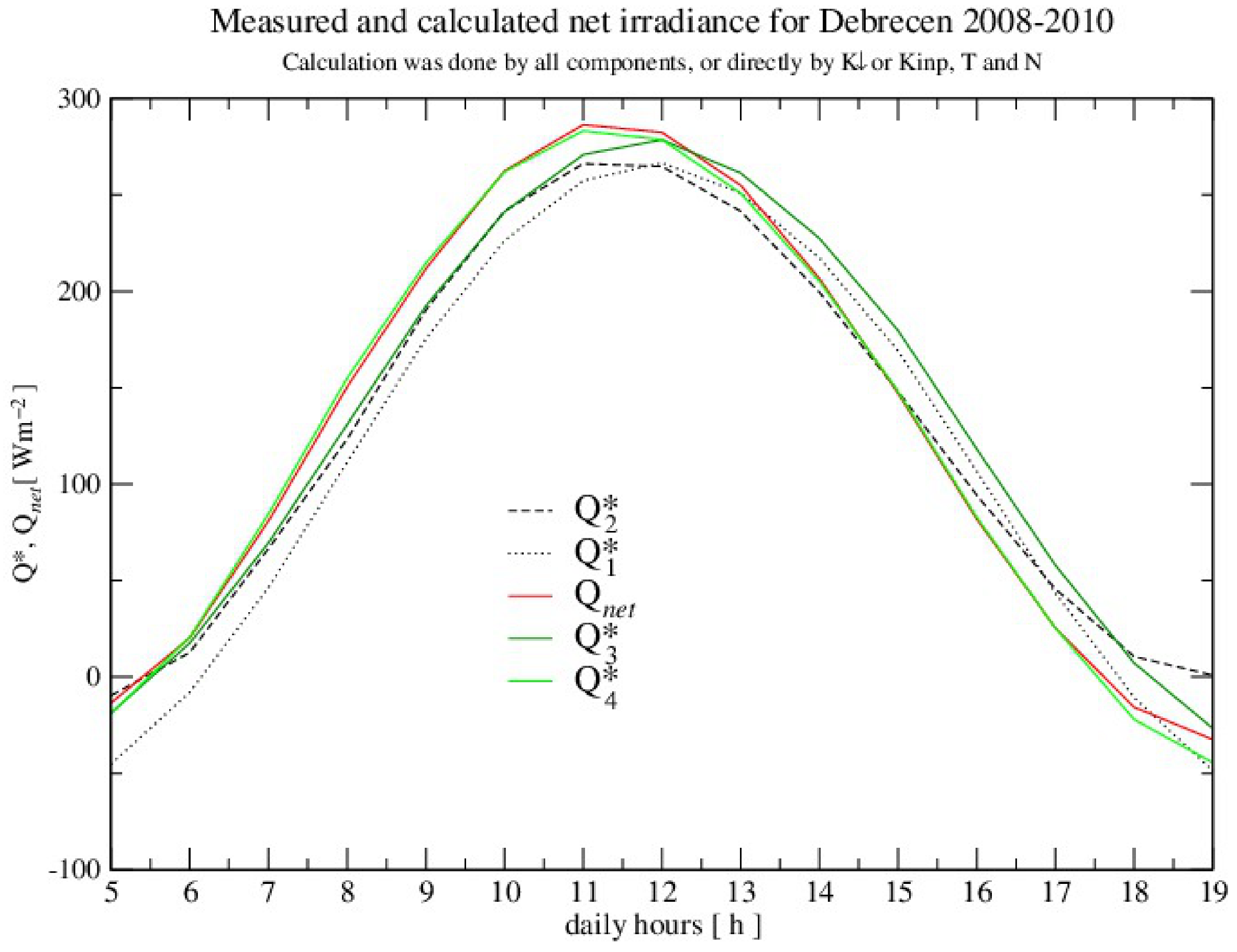
5. Assessments of Net Irradiance

The net radiation of the ground surface is given by the sum of the shortwave and longwave radiation components. However, contrary to its importance, it is very rarely included in the standard meteorological measurements. In this section, a mean annual daily variation and statistical errors for measured $Q_{net}$ and estimated $Q^{\ast }$ are discussed, where the estimated value depends on the global solar radiation, albedo, cloudiness and, in one parameterization, on the temperature. We analyze the frequently used classical parameterizations in the SVAT (Soil-vegetation-atmosphere transfer) models in the daytime ($K\downarrow >0)$ and in the nighttime ($K\downarrow =0)$ separately for a better understanding of the accuracy of the parameterizations in the Pannonian Basin.

5.1. Daytime

To estimate the net irradiance ($Q^{\ast }$, (W m⁻²)) from the routine meteorological measurements, an empirical equation was taken, such as Holtslag and Van Ulden [5].

$$Q_H^{\ast }=0.9\frac{\left(1-A\right)·K\downarrow +c_1{T}^6-\sigma T^4+c_2(N/8)}{\left(1+c_3\right)}$$

(22)

where $T$: atmospheric temperature (K) from a 2-m measuring height, $\sigma$: the Stefan–Boltzmann constant ($\sigma =5.670·{10}^{-8}{ \mathrm{W} \mathrm{m}}^{-2 }{K}^{-4}$), $c_1=5.3·{10}^{-13}{ \mathrm{W} \mathrm{m}}^{-2}{ K}^{-6}$, $c_2=60{ \mathrm{W} \mathrm{m}}^{-2}$ and $c_3=0.12$. In this equation, we used calculations for Holtslag’s clear sky calculations and changed both the cloudiness corrections and both albedos to obtain the statistical errors. Besides that, the empirical equation following the idea of Göckede and Foken [14] was used. They used the global solar irradiance as an input parameter [11].

$$Q_F^{\ast }=0.9·K_{inp}·\left(1-A-\frac{0.08·\rho ·c_p}{K_{0F}}\right)$$

(23)

In this equation $K_{inp}$ is the measured global solar irradiance and can be substituted with $K\downarrow$, $A$ is albedo, as earlier, $K_{0F}\downarrow$ is described in Section 2 and Section 4.1 as the downwelling solar radiation for clear sky situations based on Foken [11] and $\rho$ is the air density (kg m⁻³). Based on the ideal gas low,

$$\rho =\frac{p·100}{R_d·T_v}$$

(24)

where $p$ measures the station pressure in (hPa), $R_d=287.06 {\mathrm{J} \mathrm{kg}}^{-1}{ K}^{-1}$ is the specific gas constant for the dry air and $T_v$ is the virtual temperature in (K).

$$T_v=T\left(1+0.608·q\right)$$

(25)

where $q$ is the specific humidity (kg kg⁻¹) that is calculated as $q=0.622·\frac{e}{p-0.378·e}$, where $e$ is the water vapor pressure in the same unit as the pressure (hPa), which is calculated based on the relative humidity ($Rh)$ and the saturated water vapor pressure ($e_s$) in the temperature, $T,$ is calculated as follows:

$$e_s\left(T\right)=\frac{17.62·T}{243.12+T}$$

(26)

for water and

$$e_s\left(T\right)=\frac{22.46·T}{272.162+T}$$

(27)

for ice.

The water vapor pressure is calculated as $e=e_s·Rh/100$, and finally, we give the formula of the specific heat of moist air at a constant pressure: $c_p=1004.67·\left(1+0.84·q\right)$ (J kg⁻¹ K⁻¹).

Furthermore, we compared Holtslag and Van Ulden [5] and Foken [11] equations for $Q^{\ast }$, using measured global solar radiation and Beljaars and Bosveld [38] methodology for calculation of the albedo.

The following statistical errors are calculated and shown in

Table 9. Statistical errors and percentages of cases in which the relative errors were smaller than 25% (R_err < 25%) in the calculations of the net irradiance, $Q^{\ast }$. We used the next symbols in the table: Foken [11] net radiation model $Q_F^{\ast }$ and Holtslag and Van Ulden [5] net radiation model $Q_H^{\ast }$. The low index used $K_{inp}$ for the measured global solar radiation and $Fkc$, $Fbg$, $Hkc$ and $Hbg$ for its assessment depending on Foken’s or Holtslag’s clear sky calculation and cloudiness correction. ${Aee}^{\prime }$ represent the Nyren and Gryning [37] and $Abb$ Beljaars and Bosveld [38]-type parameterizations of albedo. The second column inside the main columns represents statistical errors of the net radiation but only for period with high solar elevation when the estimated sensible heat flux based on De Bruin and Holtslag [10] was positive. Gray—methods with higher correlation coefficients.

Net Irradiance	BIAS (W m−2)		MAE (W m−2)		RMSE (W m−2)		Correlation Coefficient		Rerr < 25% (%)
$Q_{{F FkcAee}^{\prime }}^{\ast }$	−25	−35	42	73	61	102	0.93	0.80	41	84
$Q_{{F FbgAee}^{\prime }}^{\ast }$	−25	−37	41	75	61	97	0.93	0.81	31	82
$Q_{{H HkcAee}^{\prime }}^{\ast }$	−24	−22	43	72	65	100	0.92	0.84	52	74
$Q_{{H HbgAee}^{\prime }}^{\ast }$	−24	−24	42	74	63	100	0.92	0.83	51	73
$Q_{F K_{inp}{Aee}^{\prime }}^{\ast }$	−23	−28	29	34	38	46	0.98	0.98	59	97
$Q_{F FkcAbb}^{\ast }$	−18	0	40	67	61	94	0.94	0.83	50	71
$Q_{F FbgAbb}^{\ast }$	−17	−4	40	67	57	90	0.93	0.84	50	72
$Q_{H HkcAbb}^{\ast }$	−12	−10	43	72	64	98	0.92	0.81	50	69
$Q_{H HbgAbb}^{\ast }$	−22	−21	40	67	59	93	0.93	0.84	52	75
$Q_{F K_{inp}Abb}^{\ast }$	−15	1	25	21	32	26	0.99	0.99	58	93
$Q_{H K_{inp}Abb}^{\ast }$	−13	−5	30	34	37	41	0.98	0.97	55	84
$Q_{H K_{inp}{Aee}^{\prime }}^{\ast }$	−22	−14	32	39	40	49	0.97	0.96	55	86

: BIAS, MAE and RMSE, together with the percentage of cases in which the relative errors were fewer than 25% (R_err < 25%) for the calculation for clear sky global solar radiation, cloudiness calculations and albedo, where albedo ${Aee}^{\prime }$ does not depend on the cloudiness, whereas $Abb$ does. The second numbers in the column represent statistical errors of the net radiation but only for periods with high solar elevation when the sensible heat flux ($H$) was positive. The moment when the sensible heat flux changed its direction was calculated, according to De Bruin and Holtslag [10], from equation:

$$H=\frac{\frac{\gamma }{S_c}·\left(Q^{\ast }-Q_g\right)}{1+\frac{\gamma }{S_c}}+\beta$$

(28)

where $\beta =20 {\mathrm{W} \mathrm{m}}^{-2}$ is the constant, $Q_g$ is the ground heat flux transported into the soil, $s_c=\partial e_s/\partial T$ and the psychometrics constant is $\gamma =c_p/\lambda$, where λ is the latent heat of vaporization. The rough estimation of the ground heat flux transported into the soil is $Q_g=0.1·Q^{\ast }$ [70]. There are a few approximated relationships between $S_c$ and $\gamma$ [11,12,37]. We checked all the approximations in our dataset and chose the second method [12].

Although a significant difference is not noticed between Holtslag and Van Ulden [5] and Foken [11] calculations for net radiations, or between Kasten and Czeplak [39] and Burridge and Gadd [40] mathematics for cloudiness, it is clear that the inclusion of cloudiness in the calculation of albedo, as recommended in Beljaars and Bosveld [38], improves the estimation of net radiation. It is obviously confirmed that the inclusion of measured global solar irradiance, as suggested in Göckede and Foken [14], significantly improved the previous estimations of net radiation when these measurements were not available, as is expected.

Furthermore, describing a successful estimation of net radiation can help the estimation of daytime sensible heat flux from routine meteorological measurements. It is especially useful at locations where special profile or flux measurements do not exist. In addition, these methods can be very useful tools for data quality control for special micrometeorological measurements.

5.2. Nighttime

The nighttime net thermal radiation depends on the temperature and cloudiness. We used an equation that was adapted from Burridge and Gadd [40]:

$$Q^{\ast }=Q_{ref}^{\ast }·{\left(\frac{T}{T_{ref}}\right)}^4·\left(1-0.9·N_{eff}\right)$$

(29)

where $T$ is the measured temperature at a 2-m height (K), $T_{ref}=285 K$, $Q_{ref}^{\ast }=-91 {\mathrm{W} \mathrm{m}}^{-2}$ and $N_{eff}=\left(N+N_{CL}\right)/16$ is the effective cloud cover, where $N$ is in octa (0, 1,…, 8).

Although nighttime net thermal radiation is not usually used for the calculation of sensible heat flux from routine measurements, we offered statistical errors for its estimation: $BIAS=-24 {\mathrm{W} \mathrm{m}}^{-2}$, $MAE=26 {\mathrm{W} \mathrm{m}}^{-2}$, $RMSE=31 {\mathrm{W} \mathrm{m}}^{-2}$ and the coefficient of correlation was 0.74. The small difference between the absolute value of $BIAS$ and $MAE$ represents a systematic underestimation, as we can see in Figure 5.

We represented only $Q_F^{\ast }$ net radiation models with Foken’s clear sky calculations, $Q_H^{\ast }$ net radiation models with Holtslag’s clear sky calculations and both models with measured $K_{inp}$, emphasizing the differences between ${Aee}^{\prime }$ and $Abb$ albedo based on Nyren and Gryning [37] and Beljaars and Bosveld [38] methodology separately. Figure 5 represents the mean annual daily variation of net radiation, which clearly confirms the facts that were discussed through statistical errors and suggests the following conclusions:

(1)

During the midday period, when sensitive heat flux is directed upwards, Foken’s calculation is clearly better than Holtslag’s calculation.

(2)

Holtslag’s method is slightly better for low solar elevation when a sensible heat flux is directed downwards.

(3)

The difference between the measured ($Q_{net}$) and calculated ($Q^{\ast }$) net irradiance is very small when we compared both methods for mathematically described cloudiness.

(4)

An albedo that includes cloudiness ($Abb$) is much better than one (${Aee}^{\prime }$) that does not.

(5)

Measured global solar radiation makes an estimation of the net irradiance significantly better in comparison to when this value is estimated.

(6)

Using the same value for global solar radiation, Foken’s estimation for net irradiance is slightly better than Holtslag’s.

(7)

The estimation of nighttime net thermal radiation is crude and has systematic errors.

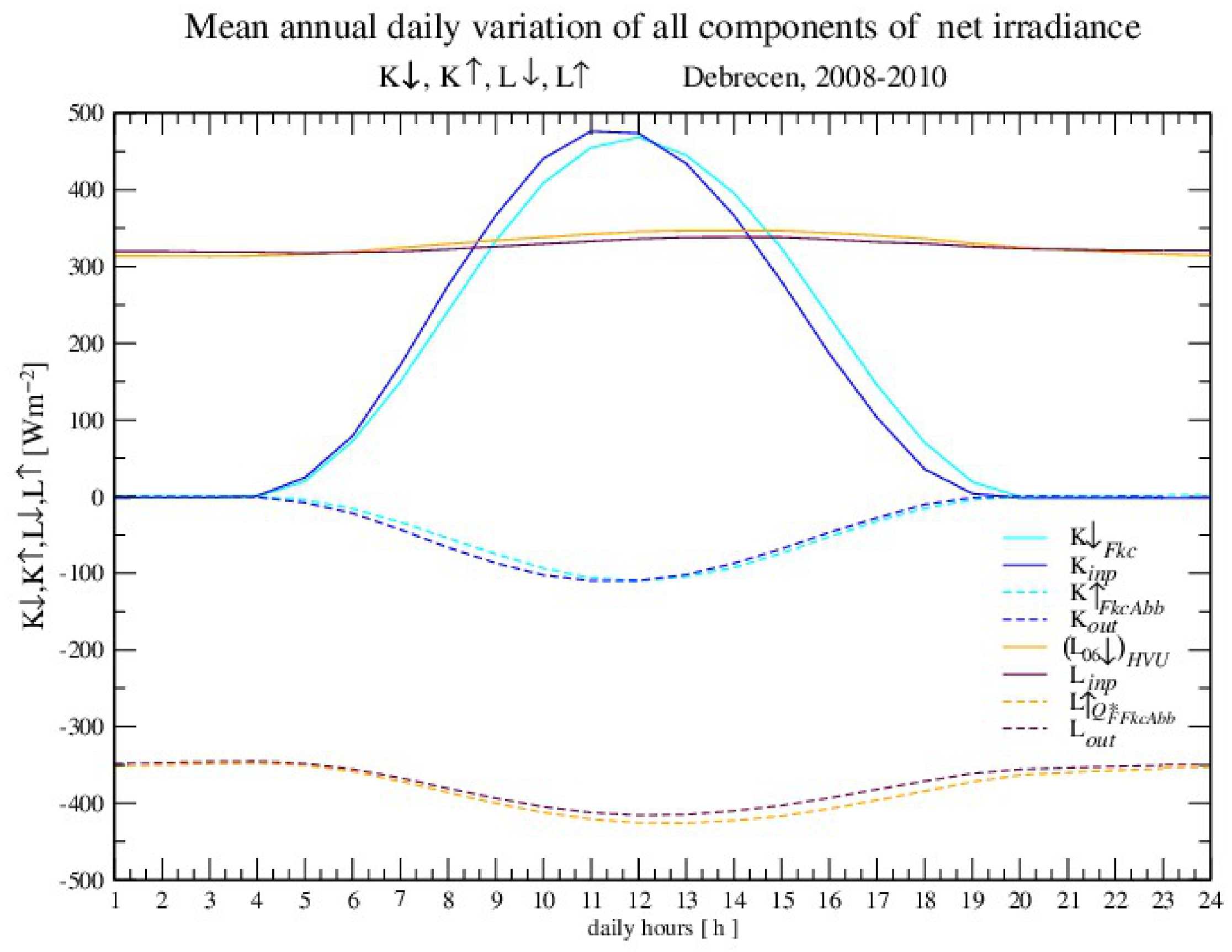
6. Assessment of Longwave Irradiance

The absorbed solar energy on the Earth’s surface is emitted into the atmosphere as upwelling LW radiation ($L\uparrow$). The part of this radiation and part of solar radiation absorbed by cloudiness and atmospheric particles and gases go back and/or forward to the Earth’s surface as downwelling LW radiation ($L\downarrow$). The fluxes of longwave radiation >4 µm are key terms in the surface energy budget and vitally important in applied meteorology. Its knowledge is essential for the forecast of frosts, fogs, temperature variations, etc. [71,72].

Although parameterization schemes for longwave radiation have their background in the irradiative transfer theory, most of them, as in the case of shortwave radiation, are based on empirical relationships derived from observed fluxes. Empirical relations usually describe LW radiation well, especially in climatic conditions similar to those from which they were derived and in clear sky conditions. Cloudiness correction, again as in the case of SW radiation, has to be included in the calculations.

6.1. Assessment of Upwelling LW Irradiance

Outgoing longwave radiation from the Earth’s surface is driven by the effective radiative, infrared surface temperature, $T_s$:

$$L\uparrow = {\epsilon }_0 \sigma T_s^4$$

(30)

where ${\epsilon }_0~0.98$ is the Earth emissivity, and $\sigma$ is Stefan–Boltzmann’s constant. $T_s$ is very rarely available from routine observations. Due to this, it is necessary to substitute this value with the screen level atmospheric temperature, $T$, which is always smaller during the day and greater during the night. Sellers [52] and Holtslag and van Ulden [5] described upwelling LW radiation using a Taylor series centered at $T$:

$$L\uparrow = {\epsilon }_0 \sigma T_s^4 {\epsilon }_0 \sigma T^4 + {\epsilon }_0 4\sigma T^3\left(T_s-T\right)$$

(31)

Since we consider the above equation over short grass, we assume ${\epsilon }_0=1$; hence, the effect of a gray body is neglected. Since $T$ feels the change of $T_s$ with a delay, especially during the day period, we used atmospheric temperature with a one-hour delay when the solar elevation was positive. For the daytime case, the last term can be approximated using either $K\downarrow$ or $Q_{net}$.

$$4\sigma T^3\left(T_s-T\right)=\mathrm{const} ·K\downarrow \vee 4\sigma T^3\left(T_s-T\right)=\mathrm{const} ·Q_{net}$$

(32)

Since more and more routine meteorological measurements are including global solar radiation, the last approximation is used more often. According to Foken [11] and Offerle et al. [53], who modified the first form of Holtslag and van Ulden [5] approximation by including albedo ($A$):

$$4\sigma T^3\left(T_s-T\right)= 0.08 K\downarrow \left(1 -A\right)$$

(33)

We also used the same mathematical expression approximated by $Q^{\ast }$ according to Holtslag and van Ulden [5]:

$$4\sigma T^3\left(T_s-T\right) = 0.12 Q^{\ast }$$

(34)

Instead of a constant 0.12 in this equation, the same authors used values that depended on atmospheric and surface conditions, especially soil moisture:

$$4\sigma T^3\left(T_s-T\right)= \frac{4\sigma T^3{R}^{,}}{\rho c_p}\left(1-c_g\right)\left(\frac{1-{\alpha }_{pt+\gamma }}{1+\gamma }\right)Q^{\ast }$$

(35)

where $\rho$ and $c_p$ were mentioned in previous sections, $\mathrm{and} R^{,}$ is the modified resistance for sensible heat flux. The default value: $R^{,}=80 {\mathrm{s} \mathrm{m}}^{-1}$, as noted in reference [5], $\gamma$ is a psychrometric constant, and ${\alpha }_{pt}$ is the Pristly–Taylor coefficient, which is a function of the soil moisture, as described in reference [73]. $c_g=0.1$ and $Q_g=c_g·Q^{\ast }$ represents the part of the net radiation that goes into the soil.

Although the soil moisture, as well as the surface soil temperature, is not part of the routine weather observations, in this paper, it is compared by measuring the outgoing LW radiation $L_{out}$ with the estimated $L\uparrow$ in a few different cases:

(a)

by Stefan–Boltzmann: $L{\uparrow }_{SB};{\epsilon }_0=1$ and $L{\uparrow }_{SB};{\epsilon }_0=0.98$

(b)

by global solar irradiance, ($K\downarrow$) and ($K_{inp}$): $L{\uparrow }_{KFkcAbb}$ and $L{\uparrow }_{K_{inp}Abb}$

(c)

by the assessment of $Q^{\ast }$: $L{\uparrow }_{Q_{F FkcAbb }^{\ast }}$ and $L{\uparrow }_{Q_{F K_{inp}Abb}^{\ast } }$

(d)

by $Q^{\ast }$ included in Equation (35): $L{\uparrow }_{Q_{F FkcAbb+{\alpha }_{PT}}^{\ast } }$ and $L{·}_{K_{inp}Abb+{\alpha }_{PT}}$

There are 7933 data hours calculated and compared. Contrary to expectations, we found that the calculations with measured $T_s$ did not have the best evaluation of $L\uparrow$. Unexpectedly, it is evident that including soil moisture measurements through ${\alpha }_{pt}$ did not improve our calculations (

Table 10. Statistical errors and coefficients of correlation for different types of models of $L\uparrow$. (The best model is shaded).

$\mathbf{Types} \mathbf{of} \mathbf{Models} \mathbf{of} \mathit{L}{\uparrow }_{ }$	AS (W m−2)	MAE (W m−2)	RMSE (W m−2)	Correlation Coefficient (r)
$L{\uparrow }_{SB}{\epsilon }_0=1$	17	17	26	0.99
$L{\uparrow }_{SB}{\epsilon }_0=0.98$	10	12	20	0.99
$L{\uparrow }_{K_{FkcAbb}}$	7	12	16	0.98
$L{\uparrow }_{K_{inp}Abb}$	7	11	15	0.98
$L{\uparrow }_{Q_{F FkcAbb}^{\ast } }$	3	8	13	0.98
$L{\uparrow }_{Q_{F K_{inp}Abb}^{\ast } }$	3	8	12	0.99
$L{\uparrow }_{Q_{F FkcAbb+{\alpha }_{PT}}^{\ast } }$	−1	14	24	0.94
$L{\uparrow }_{Q_{F K_{inp}Abb+{\alpha }_{PT}}^{\ast } }$	−13	14	22	0.96

). In that case, three numerical experiments were done: the first experiment ${\alpha }_{pt}=1.0$, the second experiment: ${\alpha }_{pt}=0.95$ from April to September and ${\alpha }_{pt}$ = 0.85 from October to March and the third experiment ${\alpha }_{pt}=0.65$. The last one was a little better than the first and the second, but it was worse than when we used the constant.

According to the assessment of upwelling LW from the routine measurements, it was compared to the Offerle et al. [53] parameterization, which used (Equation (33)) with measured $K_{inp}$ ($L{\uparrow }_{K_{inp}Abb})$ and calculated $K\downarrow$ ($L{\uparrow }_{K_{FkcAbb}}$) with Holtslag’s parameterization (Equation (34)) with $Q_F^{\ast }$, where the net radiation was calculated again with the measured $K_{inp}$ ($L{\uparrow }_{Q_{F K_{inp}Abb }^{\ast }})$ and calculated $K\downarrow$($L{\uparrow }_{Q_{F FkcAbb}^{\ast } })$. It is evident that Holtslag and van Ulden [5] parameterization with net radiation is the best in both cases: with and without measured $K_{inp}$ (Figure 6 and Table 10).

6.1.1. Assessment of Downwelling LW Irradiance for Clear Sky

In this paper, eight methods for modeling clear sky downwelling LW radiation as a function of screen level temperature, $T,$ expressed in (°K), and water vapor pressure, $e$, expressed in (hPa), are compared with measurements through statistical errors. The applied parameterizations are presented in

Table 11. Parameterizations of clear sky downwelling LW radiation, $L_{01}\downarrow$ (W m⁻²), as a function of the screen level temperature, $T,$ expressed in (°K), and water vapor pressure, $e,$ expressed in (hPa).

Model	References
$L_{01}\downarrow =\left(0.83-0.118·{10}^{-0.6·e}\right)·\sigma ·T^4$	Angström [42], recalculated 1997 for summertime in Finland (Niemelä et al. [43])
$L_{02}\downarrow =1.24·{\left(e/T\right)}^{1/7}·\sigma ·T^4$	Brutsaert [44]
$L_{03}\downarrow =\left[0.7+5.95·{10}^{-5}·\exp \left(1500/T\right)\right]·\sigma ·T^4$	Idso [45]
$L_{04}\downarrow =\left[1-\left(1+w\right)·\exp \left(-1.2+3.0·w^{1/2}\right)\right]·\sigma ·T^4$     $w=46.5 ·\left(e/T\right)$ is the precipitable water content [cm]	Prata [46]
$L_{05}\downarrow =5.31·{10}^{-13}·T^6$	Swinbank [47]
$L_{06}\downarrow =59.38+113.7·{\left(T/T_0\right)}^6+96.96·\sqrt{w/2.5}$         $T_0=273.16 \mathrm{K}$,      $w=46.5 ·\left(e/T\right)$ is the precipitable water content [cm]	Dilley and O’Brein [48]
$L_{07}\downarrow =\left\{\begin{array}{c}\left[0.72+0.009·\left(e-2\right)\right]·\sigma ·T^4 if e\ge 2 hPa \\ \left[0.72+0.076·\left(e-2\right)\right]·\sigma ·T^4 if e<2 hPa\end{array}\right.$	Niemelä et al. [43]
$L_{08}\downarrow =\left[1-0.35·\exp \left(-10·e/T\right)\right]·\sigma ·T^4$	Iziomon et al. [51]

.

There were 792 situations with clear sky conditions, 591 for the night and 201 for the day periods during the year 2009 in Debrecen. Through the statistical errors BIAS, MAE and RMSE, as well as coefficient of correlation, $r,$ Niemelä et al. [43] parameterization, $L_{07}\downarrow$, was the best (

Table 12. Statistical errors and coefficients of correlation for clear sky conditions. (all—all cases, n.—nighttime and d.—daytime). Notations are similar to Table 10. (The best model is shaded).

LW Irradiance	BIAS (W m−2)			MAE (W m−2)			RMSE (W m−2)			Correlation Coefficient (r)
	all	n.	d.
$L_{01}\downarrow$	–9	2	−13	15	12	17	21	17	22	0.93
$L_{02}\downarrow$	−16	−2	−20	18	10	20	27	18	29	0.94
$L_{03}\downarrow$	4	15	0	15	19	13	19	22	18	0.94
$L_{04}\downarrow$	−11	1	−15	15	10	17	22	16	23	0.94
$L_{05}\downarrow$	−18	2	−25	24	19	25	31	25	32	0.92
$L_{06}\downarrow$	−18	−10	−20	19	12	21	25	17	27	0.94
$L_{07}\downarrow$	–3	–8	11	14	3	17	19	19	20	0.95
$L_{08}\downarrow$	−19	−23	–7	20	23	10	26	29	19	0.94

). Similar to $L_{07}\downarrow$, similar errors have parameterizations from Idso [45], $L_{03}\downarrow$, although their errors were the smallest during the day period and almost the worst during the night, when clear sky conditions were more frequent.

6.1.2. Assessment of Downwelling LW Irradiance for All Sky Conditions

Firstly, in order to include cloudiness in our calculations, the eight parameterizations for clear sky $L_{0i, i=1, \dots ,8}\downarrow$ are combined with three different methods that describe the effects of cloudiness. The first group of parameterizations was constructed on the basis of cloudiness correction, following Niemelä et al. [43]. There are three parameterizations, where:

$${\left(L_{0i}\downarrow \right)}_{Jac}=\left(1+0.26·\frac{N}{8}\right)L_{0i, i=1, \dots , 8}\downarrow$$

(36)

$${\left(L_{0i}\downarrow \right)}_{M\&C}=\left(1+0.22·{\left(\frac{N}{8}\right)}^{2.75}\right)L_{0i, i=1, \dots ,8}\downarrow$$

(37)

Based on Jacobs [49] and Maykut and Church [50], separately. The third cloudiness correction method was for a lowland site, following Iziomon et al. [51]:

$${\left(L_{0i}\downarrow \right)}_{Izi}=\left(1+0.243·{\left(\frac{N}{8}\right)}^2\right)L_{0i, i=1,\dots ,8}\downarrow$$

(38)

All clear sky downwelling LW radiation parameterizations $(L_{0i,i=1,\dots ,8}\downarrow )$, (see Section 6.1.1) were applied in cases ${\left(L_{0i}\downarrow \right)}_{Jac}, {\left(L_{0i}\downarrow \right)}_{M\&C}$ and ${\left(L_{0i}\downarrow \right)}_{Izi}$. $\mathrm{There} \mathrm{were} \left(3·8=24\right)$ different cases for hourly downwelling LW irradiance calculations for all the sky conditions.

The downwelling LW radiation, as described by Holtslag and Van Ulden [5], was calculated using clear sky parameterizations, where the downwelling irradiance was a function of $T^6$ from Swinbank [47] and Dilley and O’Brien [48] separately:

$${\left(L_{05}\downarrow \right)}_{HVU}=5.31·{10}^{-13}·T^6+60·\frac{N}{8}\equiv L_{05}+60·\frac{N}{8}$$

(39)

$$\begin{array}{c}{\left(L_{06}\downarrow \right)}_{HVU}=59.38+113.7·{\left(T/T_0\right)}^6+96.96·\sqrt{w/2.5}+60·\frac{N}{8}\\ \equiv L_{06}\downarrow +60·\frac{N}{8}\end{array}$$

(40)

Finally, following Niemelä et al. [43], the downwelling LW irradiance was calculated for all sky conditions, with a parameterization that was developed using clear sky downwelling irradiance, cloudiness and upwelling LW irradiance:

$${\left(L_{0i}\downarrow \right)}_{Nie}=\left[1+\left(\frac{L\uparrow }{L_{0i,i=1,\dots ,8}\downarrow }-1\right)·0.87·{\left(\frac{N}{8}\right)}^{3.49}\right]L_{0i, i=1,\dots ,8}\downarrow$$

(41)

There were eight ${\left(L_{0i}\downarrow \right)}_{Nie}=\left[1+\left(\frac{L\uparrow }{L_{0i,i=1,\dots ,8}\downarrow }-1\right)·0.87·{\left(\frac{N}{8}\right)}^{3.49}\right]L_{0i, i=1,\dots ,8}\downarrow$ cases for each hour. Based on the intention to work with routine measurement data and considering the results from previous sections, the upwelling LW irradiance in Equation (41) was calculated as a function of $T$ and $Q^{\ast }$, while the net irradiance was calculated by Foken’s clear sky model, Kasten and Czeplak [39]-type cloudiness parameterizations, Beljaars and Bosveld [38] albedo and Göckede and Foken [14] calculations for net irradiance, $L{\uparrow }_{Q_{F FkcAbb}^{\ast }}.$ In general, comparing by the statistical errors only for cloudiness correction, we concluded that the Maykut and Church [50] method was slightly better than Jacobs [49]. At the same time, the cloudiness correction described by Iziomon et al. [51] was between them with: BIAS between 0 W m⁻² for ${\left(L_{04}\downarrow \right)}_{Izi}$ and 17 W m⁻² for ${\left(L_{03}\downarrow \right)}_{Izi}$, MAE between 18 W m⁻² for ${\left(L_{06}\right)}_{Izi}$ and 26 W m⁻² for ${\left(L_{05}\downarrow \right)}_{Izi}$, RMSE between 22 W m⁻² for ${\left(L_{06}\downarrow \right)}_{Izi}$ and 32 W m⁻² for ${\left(L_{05}\right)}_{Izi}$ and a correlation coefficient 0.91 for almost all parameterizations except ${\left(L_{01}\downarrow \right)}_{Izi} \mathrm{and} {\left(L_{05}\downarrow \right)}_{Izi}, \mathrm{which} \mathrm{were} \mathrm{less}$. Slightly better statistical errors than all three above-mentioned assessments of downwelling LW irradiance were described by Niemela et al. [43] and shown in the grey column of

Table 13. Statistical errors for all sky conditions. Each error is represented in three separated columns for Jacobs [49], Maykut and Church [50] cloudiness and for Niemelä et al. [43] parameterization. Shown errors are calculated in 2$·8+8=24$ cases. In the last two rows, we show Holtslag and Van Ulden [5] cloudiness corrections with Swinbank [47] ${\left(L_{05}\downarrow \right)}_{HVU}$ and with Dilley and O’Brien [48] ${\left(L_{06}\right)}_{HVU}$ parameterizations (gray belt, best solution).

LW Irradiance	BIAS (W m−2)			MAE (W m−2)			RMSE (W m−2)			Correlation Coefficient (r)
	Jac	M&C	Nie	Jac	M&C	Nie	Jac	M&C	Nie	Jac	M&C	Nie
($L_{01}\downarrow$)…	6	−1	2	18	17	16	24	22	24	0.88	0.90	0.88
($L_{02}\downarrow$)…	−3	−8	−1	21	21	17	27	27	25	0.89	0.91	0.90
($L_{03}\downarrow$)…	31	−13	10	34	21	18	42	27	25	0.90	0.92	0.90
($L_{04}\downarrow$)…	13	−3	1	24	18	16	31	23	23	0.90	0.91	0.90
($L_{05}\downarrow$)…	5	−11	−2	28	26	20	35	32	28	0.87	0.88	0.88
($L_{06}\downarrow$)…	6	−10	−4	18	18	18	24	22	23	0.90	0.92	0.88
($L_{07}\downarrow$)…	3	−12	−4	22	20	17	28	26	24	0.90	0.92	0.89
($L_{08}\downarrow$)…	22	5	6	29	20	18	38	26	25	0.90	0.91	0.90
${\left(L_{05}\downarrow \right)}_{HVU}$	−3			24			28			0.87
${\left(L_{06}\downarrow \right)}_{HVU}$	−2			15			19			0.91

.

The number of hours with absolute errors greater than 100 W m⁻² for Niemelä et al. [43] parameterization was very stable and varied between 24 for Dilley and O’Brien [48] to 29 for Swinbank [47] and Iziomon et al. [51] clear sky downwelling LW parameterization. According to the relative errors, it was noticed that, for almost all parameterizations, the relative errors were smaller than 25%. However, in order to distinguish slight differences between them, percentages for the relative errors smaller than 10% are offered in

Table 14. Number of situations in percentages (%), with relative errors (R_err) smaller than 10%. Columns represent: $\left(L_{0i, i=1,\dots ,8}\downarrow \right)$, respectively, as in Table 11. Rows represent cloudiness corrections: Jacobs [49], Maykut and Church [50], Niemelä et al. [43] and Holtslag and Van Ulden [5]-type corrections $\left(60·\frac{N}{8} {\mathrm{W} \mathrm{m}}^{-2}\right),$ which work only with $L_{CL5}\downarrow$ and $L_{CL6}\downarrow .$ For cloudiness corrections, these abbreviations are used for the ($L_{0i}$) index: Jacobs (Jac), Maykut and Church (M&C), Niemelä (Nie) and Holtslag and Van Ulden (HVU), respectively.

$\mathbf{Rerr}({\mathit{L}}_{0\mathit{i}}\downarrow ) < 10\% (\%)$ Method	${\mathit{L}}_{01}\downarrow$	${\mathit{L}}_{02}\downarrow$	${\mathit{L}}_{03}\downarrow$	${\mathit{L}}_{04}\downarrow$	${\mathit{L}}_{05}\downarrow$	${\mathit{L}}_{06}\downarrow$	${\mathit{L}}_{07}\downarrow$	${\mathit{L}}_{08}\downarrow$
Jacobs	73%	70%	57%	73%	65%	81%	76%	66%
Maykut & Church	85%	77%	80%	84%	67%	87%	77%	65%
Niemelä	87%	85%	85%	86%	80%	87%	85%	86%
Holtslag and Van Ulden					85%	90%

. The columns represent different clear sky parameterizations, while the rows represent additional cloudiness corrections.

Comparing the 7933 h of observations with all the sky conditions during the year 2009, we concluded that Dilley and O’Brien [48] parameterizations with Holtslag and Van Ulden [5] cloudiness corrections had the smallest statistical errors (Table 14, grey belt, ${\left(L_{06}\downarrow \right)}_{HVU}$). It is noticeable for the downwelling irradiance, according to Niemelä et al. [43], that all sky cloudiness conditions, together with Dilley and O’Brien [48] ($L_{CL6}\downarrow$), Niemelä et al. [43] ($L_{CL1}\downarrow$), Iziomon et al. [51] ($L_{CL8}\downarrow$) or Pratta [5] ($L_{CL4}\downarrow$) parameterization of the clear sky LW irradiance, gave an excellent estimate (Table 12 and Figure 7).

7. The Statistical Errors and Validation of the Results

The stability validation of our previous results was done by comparing the statistical errors calculated for one year with the same values calculated for longer periods. Namely, we compared BIAS, MAE, RMSE and the coefficient of correlation ($r$) calculated for the year 2009 with the same errors for the two longer periods. The first period was from 2008 to 2010 and included 17,964 data hours for net radiation and 9814 data hours when $K_{inp}$ > 1 W m⁻². The second period was from 2008 to 2017 and included 61,880 data hours for LW radiation and 40,869 data hours with $K_{inp}$ > 1 W m⁻² (

Table 15. Comparison of statistical errors between the year 2009 and the periods 2008–2010 and 2008–2017 for all components of radiation using the best parameterizations: $K\downarrow$, $K\uparrow$, $L\downarrow$ and $L\uparrow$.

	BIAS (W m−2)	MAE (W m−2)	RMSE (W m−2)	Correlation Coefficient (r)	Time Periods
$K{\downarrow }_{Fkc}$	4	76	105	0.90	2008–2010
	5	71	109	0.91	2009
	4	60	96	0.93	2008–2017
$K{\uparrow }_{FkcAbb}$	−2	14	33	0.88	2008–2010
	0	16	34	0.84	2009
	−7	19	34	0.82	2008–2017
${\left(L_{06}\downarrow \right)}_{HVU}$	9	16	21	0.91	2008–2010
	−3	14	19	0.95	2009
	−1	14	19	0.92	2008–2017
$L{\uparrow }_{Q_{F FkcAbb}^{\ast }}$	7	10	15	0.98	2008–2010
	3	8	13	0.98	2009
	7	10	16	0.98	2008–2017

). We used the parameterization with the proven best results.

• Foken’s calculation for clear sky downwelling solar irradiance ($K_{0F}\downarrow$)
• Kasten and Czeplak [39] cloudiness correction for downwelling solar radiation ($K{\downarrow }_{Fkc}$)
• Beljaars and Bosveld [38] albedo ($A$) for upwelling solar irradiance ($K{\uparrow }_{FkcAbb}$)
• Foken’s equation for assessment net irradiance [11] ($Q_{F FkcAbb}^{\ast })$
• Dilley and O’Brien [48] for parameterization of clear sky downwelling LW irradiance ($L_{06}\downarrow$)
• Holtslag and Van Ulden [5] cloudiness correction for downwelling LW radiation ${\left(L_{06}\downarrow \right)}_{HVU}$
• Holtslag and Van Ulden [5] modified by Offerle [53] for the assessment of upwelling LW irradiance $\left(L{\uparrow }_{Q_{F FkcAbb}^{\ast }}\right)$

The results of the interpretation were separated, because there was the transition from manual to automatic measurements after the year 2010 at Debrecen Airport. It had the consequence of missing cloudiness measurements during the night. Namely, hours with a lack of cloudiness had to be excluded from the calculations, as well as the hours with accidentally missed data. During the period 2008–2017, there were night measurements of cloudiness only in the first half of the period—in the beginning completely and, later, only partly.

Since 2018, the measuring site Debrecen Airport WMO 12882 has been operating as a “backup” site with limited data access.

Finally, the comparison between the estimated $Q^{\ast }$ and measured $Q_{net}$ irradiance was conducted in four different cases, and the results are shown in Table 15 and

Table 16. Statistical errors and coefficients of correlation for $Q_1^{\ast }$, $Q_2^{\ast }$, $Q_3^{\ast }$ and $Q_4^{\ast }$ in Agrometeorological Observatory Debrecen for the 3-year time period from 2008 to 2010. The applied parameterizations are presented in Figure 8.

Net Irradiance	BIAS (W m−2)	MAE (W m−2)	RMSE (W m−2)	Correlation Coefficient (r)
$Q_1^{\ast }$	−20	46	66	0.93
$Q_2^{\ast }$	9	29	46	0.96
$Q_3^{\ast }$	0	37	62	0.93
$Q_4^{\ast }$.	−6	21	31	0.96

and Figure 8. These parameterizations were made directly or as the sum of all four components or irradiance: $K\downarrow$, $K\uparrow$, $L\downarrow$ and $L\uparrow$. Both parameterizations were checked using the measured variable $K_{inp}$ or using its calculated values $K{\downarrow }_{Fkc}$. (See Figure 9)

$$Q_1^{\ast }=Q^{\ast }\left(K\downarrow , N, K_0\downarrow ,T\right)=Q_{F FkcAbb}^{\ast }$$

(42)

$$Q_2^{\ast }=Q^{\ast }\left(K_{inp} K_0\downarrow ,T\right)=Q_{F K_{inp}Abb}^{\ast }$$

(43)

$$\begin{gathered} Q_3^{\ast }=K\downarrow -K\uparrow +L\downarrow -L\uparrow =Q^{\ast }\left(K\downarrow ,N, K_0\downarrow ,T, e \right)= \\ =K{\downarrow }_{Fkc}·\left(1-Abb\right)+{\left(L_{06}\downarrow \right)}_{HVU}-L{\uparrow }_{Q_{F FkcAbb}^{\ast }} \end{gathered}$$

(44)

$$\begin{gathered} Q_4^{\ast }=K_{inp}-K\uparrow +L\downarrow -L\uparrow =Q^{\ast }\left(K_{inp}, K_0\downarrow ,T,e\right)= \\ =K_{inp} ·\left(1-Abb\right)+{\left(L_{06}\right)}_{HVU}-L{\uparrow }_{Q_{F K_{inp}Abb}^{\ast }} \end{gathered}$$

(45)

Comparing statistical errors for a 10-year time period, 2008–2017, the stability of the presented calculations was clearly confirmed (

Table 17. Statistical errors and coefficients of correlation for $Q_1^{\ast }$, $Q_2^{\ast }$, $Q_3^{\ast }$ and $Q_4^{\ast }$ in Agrometeorological Observatory Debrecen for the 10-year time period from 2008 to 2017.

Net Irradiance	BIAS (W m−2)	MAE (W m−2)	RMSE (W m−2)	Correlation Coefficient (r)
$Q_1^{\ast }$	−15	36	58	0.94
$Q_2^{\ast }$	−17	27	36	0.98
$Q_3^{\ast }$	−11	37	56	0.95
$Q_4^{\ast }$.	−13	26	34	0.98

). The same statistical errors for the same variables for the time period from 2008 to 2010 are shown in Table 16 and Figure 8. It is obvious that the correlation coefficient is better for a longer period for all the variables, while the statistical errors MAE and RMSE looked clearly better only for $Q_1^{\ast }$, $Q_{2 }^{\ast }$ and $Q_3^{\ast }$.

Again, one emphasizes the significance of the measurements of global solar irradiance for the estimation of net irradiance. Namely, $Q_2^{\ast }$ and $Q_4^{\ast }$ have smaller statistical errors and better coefficients of correlation than $Q_1^{\ast }$ and $Q_3^{\ast }$, although we believe that the estimation of global solar radiation can become better if we include astronomical parameters for the EQT (Equations of Time) for our geographical location instead of $\lambda =15°$ and $\phi =50°$.

We recalculated the solar elevation angles using EQT (in minutes) from reference [74] and compared the original Foken’s [11] and Holtslag’s [5] methodology with modified Foken’s methodology through the application EQT from reference [74] in Equation (11) during the year with an hourly time step. The differences between the angles of solar elevation for this new calculation and original Foken’s methodology were much smaller compare with Holtslag’s methodology. The absolute differences were 0.84 ± 0.72° and 3.0 ± 1.6° C, respectively. We underlined the importance of the precise calculations of solar geometry.

Besides that, it was shown that net radiation ($Q^{\ast })$ is little better if it is calculated through the sum of its components than if it is calculated from the first step of parameterization—directly, Table 16 and Table 17 and Figure 9.

8. Conclusions

Comparisons of widely used parameterizations of shortwave and longwave radiation balance components in micrometeorology were provided based on the long-term measurements in the Northeastern part of the Pannonian region in Agrometeorological Observatory Debrecen. Quality-controlled datasets from WMO first-class radiation sensors were used during the time period 2008–2017.

The method for estimating the global solar irradiance ($K\downarrow$) can be used for data quality control of the measured parameters and for intercomparison tests between the global solar irradiance ($K\downarrow )$ and cloudiness $\left(N\right)$. All the methods had relative errors below 25% in around 45% of the data hours. The usual errors were connected with the short periods when the sky fast became either overcast or clear or when solar elevation was low, especially during the winter period. Individual overview of the data, synoptic situation, weather and cloudiness measurements, which were provided by Debrecen Airport (12882) 8.5 km from the Agrometeorological Observatory, are necessary in situations when the errors between the measured and calculated $K\downarrow$ are significant. In these cases, decisions can be made whether the measured or modeled data are acceptable.

Comparing nearly 62,000 h of observations with all sky conditions, we concluded that:

• Foken’s clear sky calculations [11], together with Kasten and Czeplak’s [39] methodology, are the best during unstable stratification when solar elevation is high.
• Measured global solar irradiance makes the estimation of the net irradiance significantly better in comparison to when this value is estimated.
• The estimation of nighttime net thermal irradiance is crude and has systematic errors.
• Dilley and O’Brien’s [48] clear sky parameterization with Holtslag and Van Ulden [5] cloudiness corrections had the smallest statistical errors for the estimation of downwelling longwave irradiance.
• Holtslag and Van Ulden [5] modified by Offerle [53] had the smallest statistical errors for the assessment of upwelling LW irradiance.

The method for estimating net irradiance is significant, because it is a variable that dictates the sensible heat flux and flux of the momentum when the measured surface wind is taken into consideration in the surface layer of PBL. Processes inside this layer are typically described by the laws of similarity theory, which lean on the Buckingham $\mathsf{\pi }$-theorem. The most famous of these theories of Monin–Obukhov use the mentioned fluxes to determine the characteristic turbulent length scale $L_{Mon}$ on which classes of atmospheric stability are typically based. It would be valuable to know this scale and the components of the radiation and other surface layer parameters (SLP) by the same values from the numerical models, as well as to discuss the spotted differences.

We believe that the observed differences emphasized the importance of special flux and radiation measurements in the Pannonian Plain, where the wind is weak and the duration of extremely unstable and extremely stable stratifications of PBL, which is still a discussion topic, are far more common than in Western Europe. The chosen methods can be used for data quality control and filling the gaps in these measurements.

References

1. European Communities. Harmonisation of the Pre-Processing of Meteorological Data for Atmospheric Dispersion Models; COST Action 710: Final Report; EUR 18195; Fisher, B.E.A., Erbrink, J.J., Finardi, S., Joffre, S., Morselli, M.G., Pechinger, U., Seibert, P., Thomson, D.J., Eds.; European Communities: Brussels, Belgium, 2013; p. 431. ISBN 92-828-3302-X. [Google Scholar]
2. Crawford, T.M.; Bluestein, H.B. An Operational, Diagnostic Surface Energy Budget Model. J. Appl. Meteorol. 2000, 39, 1196–1217. [Google Scholar] [CrossRef]
3. Wong, H.; Elleman, R.; Wolvovsky, E.; Richmond, K.; Paumier, J. AERCOARE: An overwater meteorological preprocessor for AERMOD. J. Air Waste Manag. Assoc. 2016, 66, 1121–1140. [Google Scholar] [CrossRef]
4. Rzeszutek, M.; Szulecka, A. Assessment of the AERMOD dispersion model in complex terrain with different types of digital elevation data. IOP Conf. Ser. Earth Environ. Sci. 2021, 642, 012014. [Google Scholar] [CrossRef]
5. Holtslag, A.A.M.; Van Ulden, A.P. A simple scheme for daytime estimates of the surface fluxes from routine weather data. J. Appl. Meteorol. Climatol. 1983, 22, 517–529. [Google Scholar] [CrossRef]
6. Beljaars, A.C.M.; Holtslag, A.A.M. Flux Parameterization over Land Surfaces for Atmospheric Models. J. Appl. Meteorol. 1991, 30, 327–339. Available online: http://www.jstor.org/stable/26186639 (accessed on 20 July 2021). [CrossRef]
7. Erbes, G.; Pechinger, U. Comparison of synoptic-based preprocessor estimates. Agric. For. Meteorol. 1999, 98–99, 509–519. [Google Scholar] [CrossRef]
8. Meyers, T.P.; Baldocchi, D.D. Current Micrometeorological Flux Methodologies with Applications in Agriculture. Micrometeorol. Agric. Syst. Agron. Monogr. 2005, 47, 381–396. Available online: http://digitalcommons.unl.edu/usdeptcommercepub/500 (accessed on 20 July 2021).
9. Foken, T. 50 Years of the Monin–Obukhov Similarity Theory. Bound. Layer Meteorol. 2006, 119, 431–447. [Google Scholar] [CrossRef]
10. De Bruin, H.A.R.; Holtslag, A.A.M. A simple parameterization of the surface fluxes of sensible and latent heat during daytime compared with the Penman-Monteith concept. J. Appl. Meteorol. Climatol. 1982, 21, 1610–1621. [Google Scholar] [CrossRef] [Green Version]
11. Foken, T. Micrometeorology; Springer: Berlin/Heidelberg, Germany, 2008; p. 305. ISBN 978-3-540-74666-9. [Google Scholar]
12. Van Ulden, A.P.; Holtslag, A.A.M. Estimation of Atmospheric Layer Parameters for Diffusion Applications. J. Clim. Appl. Meteorol. 1985, 24, 1196–1207. [Google Scholar] [CrossRef] [Green Version]
13. Holtslag, A.A.M.; De Bruin, H.A.R. Applied modeling of the nighttime surface energy balance over land. J. Appl. Meteorol. Climatol. 1988, 27, 689–704. [Google Scholar] [CrossRef] [Green Version]
14. Göckede, M.; Foken, T. Ein weitenerentwickelters Holtslag van Uldel schema zur Stabilitätsparametrisierung in der Bodenschicht. In DACH 2001, Wien. Österreichische Beiträge zu Meteorologie und Geophysik; 2001; ISSN Heft Nr. 27/Publ. Nr. 399 (CD-ROM); Available online: https://eref.uni-bayreuth.de/19623/ (accessed on 20 July 2021).
15. Foken, T. Micrometeorology; Springer: Berlin/Heidelberg, Germany, 2017; p. 362. ISBN 978-3-642-25440-6. [Google Scholar]
16. Das, Y.; Padmanabhamurty, B.; Murty, A.S.N. Some Parameterizations of Radiative Fluxes at Atmospheric Boundary Layer (ABL). J. Atmos. Pollut. 2014, 2, 1–5. [Google Scholar] [CrossRef]
17. Jiang, B.; Zhang, Y.; Liang, S.; Wohlfahrt, G.; Arain, A.; Cescatti, A.; Georgiadis, T.; Jia, K.; Kiely, G.; Lund, M.; et al. Empirical estimation of daytime net radiation from shortwave radiation and ancillary information. Agric. For. Meteorol. 2015, 211–212, 23–36. [Google Scholar] [CrossRef] [Green Version]
18. Ishola, K.A.; Mills, G.; Fealy, R.M.; Choncubhair, O.N.; Fealy, R. Improving a land surface scheme for estimating sensible and latent heat fluxes above grasslands with contrasting soil moisture zones. Agric. For. Meteorol. 2020, 294, 108151. [Google Scholar] [CrossRef]
19. Zhu, M.; Yao, T.; Yang, W.; Xu, B.; Wang, X. Evaluation of Parameterizations of Incoming Longwave Radiation in the High-Mountain Region of the Tibetan Plateau. J. Appl. Meteorol. Climatol. 2017, 6, 5833–5848. [Google Scholar] [CrossRef]
20. Liu, M.; Zheng, X.; Zhang, J.; Xia, X. A revisiting of the parametrization of downward longwave radiation in summer over the Tibetan Plateau based on high-temporal-resolution measurements. Atmos. Chem. Phys. 2020, 20, 4415–4426. [Google Scholar] [CrossRef] [Green Version]
21. Senese, A.; Maugeri, M.; Diolaiuti, G.A. Comparing Measured Incoming Shortwave and Longwave Radiation on a Glacier Surface with Estimated Records from Satellite and Off-Glacier Observations: A Case Study for the Forni Glacier, Italy. Remote Sens. 2020, 12, 3719. [Google Scholar] [CrossRef]
22. Stettz, S.; Zaitchik, B.F.; Ademe, D.; Musie, S.; Simane, B. Estimating variability in downwelling surface shortwave radiation in a tropical highland environment. PLoS ONE 2019, 14, e0211220. [Google Scholar] [CrossRef]
23. Lindauer, M.; Schmid, H.P.; Grote, R.; Steinbrecher, R.; Mauder, M.; Wolpert, B. A Simple New Model for Incoming Solar Radiation Dependent Only on Screen-Level Relative Humidity. J. Appl. Meteorol. Climatol. 2017, 56, 1817–1825. [Google Scholar] [CrossRef]
24. Acs, F.; Hantel, M. The land-surface flux model PROGSURF. Glob. Planet. Chang. 1998, 19, 19–34. [Google Scholar] [CrossRef] [Green Version]
25. Mihailovic, D.T.; Lazic, J.; Leśny, J.; Olejnik, J.; Lalic, B.; Kapor, D. A new design of the LAPS land surface scheme for use over and through heterogeneous and non-heterogeneous surfaces: Numerical simulations and tests. Theor. Appl. Climatol. 2010, 100, 299–323. [Google Scholar] [CrossRef]
26. Weidinger, T.; Nagy, Z.; Baranka, G.; Mészáros, R.; Gyöngyösi, A.Z. Determination of meteorological preprocessor for air quality models in the New Hungarian Standards. Croathian Meteorol. J. 2008, 12, 460–464. [Google Scholar]
27. Badescu, V.; Gueymard, C.A.; Cheval, S.; Oprea, C.; Baciu, M.; Dumitrescu, A.; Iacobescu, F.; Milos, I.; Rada, C. Computing global and diffuse solar hourly irradiation on clear sky. Review and testing of 54 models. Renew. Sustain. Energy Rev. 2012, 16, 1636–1656. [Google Scholar] [CrossRef]
28. Kostić, R.; Mikulović, J. The empirical models for estimating solar insolation in Serbia by using meteorological data on cloudiness. Renew. Energy 2017, 114 Pt B, 1281–1293. [Google Scholar] [CrossRef]
29. Alboteanu, I.L.; Bulucea, C.A.; Degeratu, S. Estimating Solar Irradiation Absorbed by Photovoltaic Panels with Low Concentration Located in Craiova, Romania. Sustainability 2015, 7, 2644–2661. [Google Scholar] [CrossRef] [Green Version]
30. Despotovic, M.; Nedic, V.; Despotovic, D.; Cvetanovic, S. Review and statistical analysis of different global solar radiation sunshine models. Renew. Sustain. Energy Rev. 2015, 52, 1869–1880. [Google Scholar] [CrossRef]
31. Maleki, S.A.M.; Hizam, H.; Gomes, C. Estimation of Hourly, Daily and Monthly Global Solar Radiation on Inclined Surfaces: Models Re-Visited. Energies 2017, 10, 134. [Google Scholar] [CrossRef] [Green Version]
32. Choi, Y.; Suh, J.; Kim, S.-M. GIS-Based Solar Radiation Mapping, Site Evaluation, and Potential Assessment: A Review. Appl. Sci. 2019, 9, 1960. [Google Scholar] [CrossRef] [Green Version]
33. Enríquez-Velásquez, E.A.; Benitez, V.H.; Obukhov, S.G.; Félix-Herrán, L.C.; de Lozoya-Santos, J.J. Estimation of Solar Resource Based on Meteorological and Geographical Data: Sonora State in Northwestern Territory of Mexico as Case Study. Energies 2020, 13, 6501. [Google Scholar] [CrossRef]
34. Liou, K.N. Radiation and Cloud Processes in the Atmosphere. Theory, Observation, and Modeling; United States, Oxford Monographs on Geology and Geophysics; 1992; p. 473. Available online: https://www.osti.gov/biblio/7081459 (accessed on 20 July 2021).
35. Guderian, R. (Ed.) Band 1A: Atmosphäre: Anthropogene und Biogene Emissionen—Photochemie der Troposphäre—Chemie der Stratosphäre und Ozonabbau; Springer: Berlin/Heidelberg, Germany, 2011; p. 424. ISBN 3642570879. [Google Scholar]
36. Geiger, R.; Aron, R.H.; Todhunter, P. The Climate Near the Ground; Friedrich Vieweg & Sohn Verlasges, GmbH: Brauschweig/Wiesbaden, Germany, 1995; p. 528. ISBN 978-3-322-86584-7. [Google Scholar]
37. Nyren, K.; Gryning, S.E. Nomogram for the height of daytime mixed layer. Bound. Layer Meteorol. 1999, 91, 307–322. [Google Scholar] [CrossRef]
38. Beljaars, A.C.M.; Bosveld, F.C. Cabauw Data for the Validation of Land Surface Parameterization Schemes. J. Clim. 1997, 10, 1172–1193. [Google Scholar] [CrossRef]
39. Kasten, F.; Czeplak, G. Solar and terrestrial radiation dependent on the amount and type of cloud. Sol. Energy 1980, 24, 177–189. [Google Scholar] [CrossRef]
40. Burridge, D.M.; Gadd, A.J. The Meteorological Office Operational 10 Level Numerical Weather Prediction Model (December1974); Technical Notes; British Meteorological Office: Bracknell, UK, 1974; p. 57.
41. Zheng, Z.; Wei, Z.; Wen, Z.; Dong, W.; Li, Z.; Wen, X.; Zhu, X.; Ji, D.; Chen, C.; Yan, D. Inclusion of solar elevation angle in land surface albedo parameterization over bare soil surface. J. Adv. Model. Earth Syst. 2017, 9, 3069–3081. [Google Scholar] [CrossRef] [PubMed] [Green Version]
42. Angström, A. A study of the radiation of the atmosphere. Smith. Misc. Coll. 1918, 65, 159–161. [Google Scholar]
43. Niemelä, S.; Räisänen, P.; Savijärvi, H. Comparison of surface radiative flux parameterization Part I: Longwave radiation. Atmos. Res. 2001, 58, 1–18. [Google Scholar] [CrossRef]
44. Brutsaert, W. On a derivable formula for long-wave radiation from clear skies. Water Resour. Res. 1975, 11, 742–744. [Google Scholar] [CrossRef]
45. Idso, S.B. A set of equations for full spectrum and 8- to 14-mm and 10.5- to 12.5-mm thermal radiation from cloudlessskies. Water Resour. Res. 1981, 17, 295–304. [Google Scholar] [CrossRef]
46. Prata, A.J. A new long-wave formula for estimating downward clear-sky radiation at the surface. Q. J. R. Meteorol. Soc. 1996, 122, 1127–1151. [Google Scholar] [CrossRef]
47. Swinbank, W.C. Long-wave radiation from clear skies. Q. J. R. Meteorol. Soc. 1963, 89, 339–348. [Google Scholar] [CrossRef]
48. Dilley, A.C.; O’Brien, D.M. Estimating downward clear sky long-wave irradiance at the surface from screen temperature and precipitable water. Q. J. R. Meteorol. Soc. 1998, 124, 1391–1401. [Google Scholar] [CrossRef]
49. Jacobs, J.D. Radiation climate of Broughton Island. In Energy Budget Studies in Relation to Fast-ice Breakup Processes in Davis Strait Climatological Overview; Barry, R.G., Jacobs, J.D., Eds.; Institute of Arctic and Alpine Research, Occasional Paper No. 26; University of Colorado: Boulder, CO, USA, 1978; pp. 105–120. ISSN 0069-6145. [Google Scholar]
50. Maykut, G.A.; Church, P.E. Radiation Climate of Barrow Alaska, 1962–1966. J. Appl. Meteorol. Climatol. 1973, 12, 620–628. [Google Scholar] [CrossRef] [Green Version]
51. Iziomon, M.G.; Mayer, H.; Matzarakis, A. Downward atmospheric longwave irradiance under clear and cloudy skies: Measurement and parameterization. J. Atmos. Sol. Terr. Phys. 2003, 65, 1107–1116. [Google Scholar] [CrossRef]
52. Sellers, W.D. Physical Climatology; The University of Chicago Press: Chicago, IL, USA, 1965; p. 272. ISBN 10: 0226746992. [Google Scholar]
53. Offerle, B.; Grimmond, S.B.; Oke, T.R. Parameterization of Net All-Wave Radiation for Urban Areas. J. Appl. Meteorol. 2003, 42, 1157–1173. [Google Scholar] [CrossRef]
54. Nagy, Z.; Szasz, G.; Weidinger, T.; Baranka, G.; Kovacs, N.; Decsi, A. Long term micrometeorological and energy budget measurements in Agrometeorological Observatory in Debrecen. Geophys. Res. Abstr. 2012, 14, EGU2012-8915. Available online: https://meetingorganizer.copernicus.org/EGU2012/EGU2012-8915.pdf (accessed on 20 July 2021).
55. Popov, Z.; Weidinger, T.; Baranka, G.; Nagy, Z. Assessment of net radiation from routine measurements in the Pannonian Region. In Gewex Workshop on the Climate System of the Pannonian Basin; Book of AbstractsOsijek: Osijek, Croatia, 2015; p. 53. Available online: http://www.opb.com.hr/literatura/GEWEX_Workshop_Osijek%202015_v02_20-02-2017-web.pdf (accessed on 20 July 2021).
56. Neckel, T.; Montenbruck, O. Tables. In Ahnerts Kalender für Sternfreunde; Kleines Astronomisches Jahrbuch; 52. Jahrgang Sterne und Weltraum; Hüthig GmbH: Heidelberg, Germany, 1999; ISBN 3-87973-9331. [Google Scholar]
57. Göckede, M. Das Windprofil in den Untersten 100 m der Atmosphäre unter Besonderer Berücksichtigung der Stabilität der Schictung. Master’s Thesis, Universitat Bayreuth, Bayreuth, Germany, 2000; p. 133. [Google Scholar]
58. Younes, S.; Muneer, T. Comparison between solar radiation models based on cloud information. Int. J. Sustain. Energy 2007, 26, 121–147. [Google Scholar] [CrossRef]
59. Didari, S.; Zand-Parsa, S. Estimation of daily global solar irradiation under different skyconditions in central and southern Iran. Theor. Appl. Climatol. 2017, 127, 587–596. [Google Scholar] [CrossRef]
60. Pietras-Szewczyk, M. A GIS Open Source Software Application for Mapping Solar Energy Resources in Urban Areas. E3S Web Conf. 2019, 116, 00060. [Google Scholar] [CrossRef]
61. Stull, R.B. An Introduction to Boundary Layer Meteorology; Kluwer Academic Publishers: Dordrecht, The Netherlands, 1988; p. 670. ISBN 978-94-009-3027-8. [Google Scholar]
62. Liston, G.E.; Itkin, P.; Stroeve, J.; Tschudi, M.; Stewart, J.S.; Pedersen, S.H.; Reinking, A.K.; Elder, K. A Lagrangian snow-evolution system for sea-ice applications (SnowModel-LG): Part I—Model description. J. Geophys. Res. Oceans 2020, 125, e2019JC015913. [Google Scholar] [CrossRef]
63. Marsh, C.B.; Pomeroy, J.W.; Wheater, H.S. The Canadian Hydrological Model (CHM) v1.0: A multi-scale, multi-extent, variable-complexity hydrological model—Design and overview. Geosci. Model Dev. 2020, 13, 225–247. [Google Scholar] [CrossRef] [Green Version]
64. Warren, S.G.; Eastman, R.M.; Hahn, C.J. A Survey of Changes in Cloud Cover and Cloud Types over Land from Surface Observations, 1971–1996. J. Clim. 2007, 20, 717–738. [Google Scholar] [CrossRef] [Green Version]
65. World Meteorological Organization. Guide to Meteorological Instruments and Methods of Observation; CIMO Guide, 2014: World Meteorological Organization (2014) Obseration of Clouds. (WMO-No.8); World Meteorological Organization: Geneva, Switzerland, 2014; Chapter 15, p. 1128; Available online: http://hdl.handle.net/11329/365 (accessed on 20 July 2021).
66. Paltridge, G.W.; Platt, C.M.R. Radiative Processes in Meteorology and Climatology; Elsevier: Amsterdam, The Netherlands, 1976; p. 318. ISBN 10:0444414444. [Google Scholar]
67. De Rooy, W.C.; Holtslag, A.A.M. Estimation of Surface Radiation and Energy Flux Densities fromSingle-Level Weather Data. J. Appl. Meteorol. 1999, 38, 526–540. [Google Scholar] [CrossRef]
68. Iziomon, M.G.; Mayer, H.; Matzarakis, A. Empirical Models for Estimating Net Radiative Flux: A Case Study for Three Mid-Latitude Sites with Orographic Variability. Astrophys. Space Sci. 2000, 273, 313–330. [Google Scholar] [CrossRef]
69. Duynkerke, P.G. The roughness length for heat and othervegetation parameters for a surface of short grass. J. Appl. Meteorol. 1992, 31, 579–586. [Google Scholar] [CrossRef] [Green Version]
70. Holtslag, A.A.M. Surface Fluxes and Boundary Layer Scaling Models and Applications; Scientific Report WR 87-2 of the Royal Netherlands Meteorological Institute; Royal Netherlands Meteorological Institute: De Bilt, The Netherlands, 1987; p. 185.
71. Kleczek, M.A.; Steeneveld, G.-J.; Holtslag, A.A.M. Evaluation of the Weather Research and Forecasting Mesoscale Model for GABLS3: Impact of Boundary-Layer Schemes, Boundary Conditions and Spin-Up. Bound. Layer Meteorol. 2014, 152, 213–243. [Google Scholar] [CrossRef]
72. Lábó, E.; Geresdi, I. Numerical modeling of the transfer of longwave radiation in water clouds. Időjárás 2019, 123, 147–163. [Google Scholar] [CrossRef]
73. Agam, N.; Kustas, W.P.; Anderson, M.C.; Norman, J.M.; Colaizzi, P.D.; Howell, T.A.; Prueger, J.H.; Meyers, T.P.; Wilson, T.B. Application of the Priestley–Taylor Approach in a Two-Source Surface Energy Balance Model. J. Hydrometeorol. 2010, 11, 185–198. [Google Scholar] [CrossRef]
74. Iqubal, M. An Introduction to Solar Radiation; Academic Press: Don Mills, ON, Canada, 1983; p. 390. ISBN 0-12-373750-8. [Google Scholar]
Figure 1. Micrometeorological (radiation, surface energy budget and profile) measurements in the Agrometeorological Observatory Debrecen. (a) Temperature, relative humidity and wind speed profile measurements on a 10-m tower; (b) Eddy covariance measurements on a 4-m tower; (c) radiation balance components and surface temperature measurements with WMO first class instruments (small photo with a Kipp&Zonen CGR4 pyrgeometer) and (d) Debrecen, Novi Sad and Belgrade locations in the Pannonian Basin.
Atmosphere 12 00935 g001
Figure 2. (a) Shortwave downwelling solar irradiance for a clear sky obtained by Holtslag’s and Foken’s clear sky calculations for 2009 (upper panel) and (b) during 201 h in chronological order with clear sky conditions in Agrometeorological Observatory Debrecen. The red line represents the measurements (in the middle). (c) Comparison between the measured and calculated K 0 for four clear sky days in different periods of the year (lower panels).
Atmosphere 12 00935 g002aAtmosphere 12 00935 g002b
Figure 3. Comparisons between the measurements and four models for the calculation of global solar irradiance can be seen with the (a) mean annual daily variations of the global solar irradiance. (b) The hours with the greatest errors.
Atmosphere 12 00935 g003
Figure 4. Comparisons between the measurements ( K o u t ) and two models for the calculation of shortwave reflected solar irradiance (a) (green line) albedo calculations based on the Nyren and Gryning [37] model, K F k c A e e and (b) (violet line) using Beljaars and Bosveld [38] methodology, K F k c A b b . Foken’s calculations for clear skies and Kasten and Czeplak [39]-type cloud parameterization was used for the global solar radiation calculations.
Atmosphere 12 00935 g004
Figure 5. Mean annual daily variation of net irradiance Q . Notation similar to Table 8.
Atmosphere 12 00935 g005
Figure 6. Mean annual daily variation of L for four models and measurements. Models that used routine meteorological measurements included, separately: K F k c or K i n p . Abbreviations of the models are same as in Table 9.
Atmosphere 12 00935 g006
Figure 7. Mean annual daily variation of all modeled sky downwelling LW irradiance Niemelä et al. [43] combined with all the clear sky parameterizations ( L 0 i ,   i = 1 , , 8 ) (W m−2) described in Section 6.1.1 are represented with black and grey lines and marked from L 01 N i e in Table 8. Two parameterizations: (   L 05 H V U and L 06 H V U ) based on Holtslag and Van Ulden [5] are represented in colored lines. See, also, Table 11, Table 12 and Table 14.
Atmosphere 12 00935 g007
Figure 8. Mean annual daily variations of the measured Q n e t and calculated net irradiances: Q 1   , Q 2 , Q 3 and Q 4   .
Atmosphere 12 00935 g008
Figure 9. Mean annual daily variations of all four components of the radiation balance. The components are measured and calculated from routine meteorological measurements and observations: K F k c ,   K i n p , K F k c A b b   ,   K o u t , L 06 H V U ,   L i n p , L Q F   F k c A b b   and   L o u t .
Atmosphere 12 00935 g009