Abstract
Though the traditional convolutional neural network has a high recognition rate in cloud classification, it has poor robustness in cloud classification with occlusion. In this paper, we propose a novel scheme for cloud classification, in which the convolutional neural networks are used for feature extraction and a weighted sparse representation coding is adopted for classification. Three such algorithms are proposed. Experiments are carried out using the multimodal ground-based cloud dataset and the results show that in the case of occlusion, the accuracy of the proposed methods can be much improved over the traditional convolutional neural network-based algorithms.
1. Introduction
Recently, with the expansion of big data combined with the improvement in algorithms and the exponential growth in computing power, machine learning has become a research highlight. Machine learning, especially deep learning, is widely used in computer vision, speech recognition, natural language processing, data mining and meteorological information processing.
In the early days, Buch et al. extracted features from cloud images, including texture measurements, location information and pixel brightness, then used binary decision trees to divide them into four kinds of clouds: altocumulus, cirrus, cumulus and stratiform []. Singh et al. proposed a procedure to test the texture feature used for the automatic training of a cloud classifier, in which five feature extraction methods were examined, namely autocorrelation, co-occurrence matrix, edge frequency, Law’s feature and primitive length. These tests can help us better understand the advantages and disadvantages of different feature extraction methods and classification techniques []. Heinle et al. made use of k-nearest neighbor classifier to distinguish 7 kinds of cloud images by extracting color and texture features from cloud images []. Neto et al. used the multivariate color space features to classify clouds and sky pixels using the statistical features of Euclidean geometric distance []. Liu et al. proposed a multiple random projection algorithm to obtain textons and discriminative features []. However, the accuracy of these cloud classification methods based on manual feature extraction is far from expectation, and we must manually design features carefully for each classification.
Cloud classification plays a key role in a wide range of applications such as solar power generation, weather forecasting [,], deep space climate observatory mission [], rainfall estimation [] and optical remote sensing []. However, cloud classification is a challenging task. Different clouds show different meteorological information features such as temperature, humidity, pressure, wind speed and color distribution. To achieve cloud classification, it is necessary to accurately estimate its characteristics from the shape, thickness, degrees of sparseness and other cloud features. However, the traditional cloud classification [,,] is in the charge of professional observers. In addition to consuming a lot of labor, there will also be human errors, and it is more difficult to classify the clouds with a satisfactory accuracy when there exist interferences such as sunlight, fog and many others.
Recently convolution neural networks (CNN) have been widely used in image classification and recognition applications. Such networks have many advantages. First, they do not need to extract features manually. In fact, the CNNs automatically extract features through many training pictures and yield a very good performance. Secondly, they can process many data well. Moreover, they can also reflect a strong image discrimination under a large amount of data, so they are a good choice for dealing with the ever-changing clouds. Yang et al. proposed CNN model, known as LeNet-5, yielding an accuracy of handwritten digit recognition as high as 99% []. Krizhevsky proposed a deep neural network model, denoted as Alexnet, which is relatively smaller than the LeNet in size, and changed the sigmoid activation function to a simpler ReLU activation function. Such a model makes the training easier under different parameter initialization methods and can reduce overfitting by dropout layers []. In [], an efficient network, called Inception-v3, was proposed, but the deeper network is more difficult to train. He et al. proposed a residual learning framework to simplify the training of deeper networks and the network, denoted as ResNet, takes the residual blocks as the basic blocks and can prevent gradient from disappearing []. Liu et al. used multimodal information and visual features to achieve cloud classification through support vector machine [], where a fusion of convolutional neural networks, including visual sub-network and multimodal sub-network, is proposed. After extracting visual and multimodal features, a weighted integration was used for cloud classification []. Although the recognition accuracy of these CNN-based cloud classification methods is very high, they have a common weak point—lack of robustness to perturbation.
Compressed sensing (CS) [,] is a recently developed technology. It is based on the concept of sparse representation of signals []. Let be a signal vector. It is called -sparse in a matrix if , where D is called the dictionary and denotes the number of non-zero entries in the coefficient vector . Sparse representation has been used in the fields of image processing [] and face recognition [,]. A weighted sparse representation was proposed in [] and simulations show that it is more robust to occlusion, destruction and other interferences. Gan et al. [] proposed a dual norm bounded sparse coding, which classifies cloud images by extracting nine-dimensional features, including five color features and four statistical features, but they did not execute the robustness analysis.
In this paper, we investigate classification of ground-based clouds that are observed by ground-based cameras. The main contributions of this paper are as follows:
- A novel structure for robust cloud classification is proposed, in which the features are extracted by convolution neural networks and the classification is executed using the weighted sparse representation;
- A two-channel-neural network is proposed for extracting features of the ground-based clouds.
Experimental results show that our proposed method yields a satisfactory performance for classifying ground-based clouds. In particular, the robustness of the proposed two-channel-neural network-based classifier is better than the one with a single convolutional neural network in the case of less occlusion.
The rest of this paper is organized as follows: in Section 2, we briefly introduce some related work, we describe a novel robust cloud classification structure and specific algorithm flow in Section 3, Section 4 presents experimental analysis. To end this paper, some remarking points are given in Section 5.
2. Related Work
Now, we introduce some existing results that will be used for our proposed robust classification algorithm for ground-based clouds.
2.1. ResNet Model
It has been observed that after adding too many layers in a CNN, the training error tends to rise. Though the numerical stability brought by the batch normalization makes it easier to train deeper networks, this problem still exists. The ResNet is proposed for addressing this problem. The residual block is the basic block of the ResNet. In a residual block, the input can propagate forward faster through cross layer data lines, and the occurrence of gradient disappearance can be reduced. Two additional major benefits of rectified linear units(ReLU) are sparsity and a reduced likelihood of vanishing gradient [], see Figure 1.
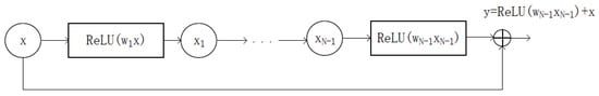
Figure 1.
Flowchart of a residual block in the ResNet, where x is the input data vector and y is the output vector, while ReLU is rectified linear units: ReLU(z) = Max (0,z).
Table 1 shows the parameters involved in the ResNet-50 model.

Table 1.
Architecture of the ResNet-50, c is the number of channels, m × n is the dimension of data, k × k is convolution kernel size.
2.2. Inception Model
The efficient convolutional neural network based on Inception model, proposed in [], consists of a set of basic convolution blocks, i.e., the Inception blocks. The naive version of such a network is showed in Figure 2.
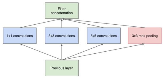
Figure 2.
Block-diagram of the Inception CNN—a naive version.
As shown in Figure 2, the k × k convolutions, for k = 1, 3 and 5 (k is 2D of convolution kernel sizes), are employed to extract information in different spatial sizes. However, this structure increases in the number of outputs from stage to stage [].
The Inception module with dimension reduction is shown in Figure 3, where the convolutions are used to compute reductions before the expensive and convolutions. Besides being used for dimension reduction, they are also used for the rectified linear activation, which makes them dual-purpose.
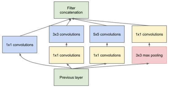
Figure 3.
Block-diagram of the Inception module with dimension reduction.
In general, an Inception network is a network consisting of modules of the above type, stacked upon each other with occasional max-pooling layers with stride 2 to halve the resolution of the grid and therefore, reducing the computational complexity and improving performance [].
Table 2 shows the parameters involved in the Inception-v3 model.
Table 2.
Architecture of the Inception-v3, c is the number of channels, m × n is the dimension of data, k × k is convolution kernel size.
2.3. Robust Sparse Coding-Based Classification
The traditional sparse coding problem is formulated as
where is the prescribed sparsity level. This coding model actually assumes that the coding residuals follow Gaussian or Laplacian distribution.
When applied for image recognition, each image is represented by a (feature) vector and the columns of the dictionary are formed with the m training images and it is assumed that the test images y can be well represented as a linear combination of training samples with a few terms involved, i.e., not more than as (1) suggested.
In practice, the residual may be far away from Gaussian distribution or Laplacian distribution, especially when the images contain occlusion or damage, so the traditional sparse coding model has a poor robustness. To improve the robustness, we must make a good use of those pixels which are not perturbed and neglect those greatly distorted in the sparse coding-based classification (1). This can be done by assigning each pixel as weighting factor, leading to the following robust sparse coding problem:
where the diagonal matrix W is selected based on the residual vector in such a way that if , then . Here, we choose W with
where the parameters are determined by experiments []. Usually, W is normalized . See the next section.
The class that image y belongs to, denoted as , is then determined by
3. Our Proposed Methods
We propose a novel robust classification scheme for ground-based clouds. The basic idea is to use CNNs for feature extraction and sparse coding for classification.
3.1. A Two-Channel-Neural Network-Based Feature Extraction
A more sophisticated approach is depicted in Figure 4, which contains two parts. The first one is for feature extraction, which converts an image into a (feature) vector z. The second part is for classifying the feature vector z.
As each CNN performs differently for different set of conditions, an intuitive idea is to fuse the features obtained with more than one CNNs. Here, we propose a scheme, shown in Figure 4, where two CNNs are used, yielding feature vectors for that are simply stacked as
Let . The system of feature selection aims to convert the feature vector y of dimension into a vector z of dimension n. Here, we propose such a system consisting of two projections and :
where the two projections and are determined with the training samples with —data matrix and with —mean matrix of the kth class for .
- —For a given , denote the mean and variance vectorsDefine , which is a vector determined by the matrix Y with (7). Let with for be the set of the smallest entries of , then the projection such that is given byThus, for , i.e., . As understood, the projection intends to keep those entries of the feature vector y, which are clustered within the each of the classes.
- —With obtained, we can compute the mean and variance vectors, liked as , using (7). Let with for be the set of the n largest entries of , then the projection such that is given byUnlike , aims at enhancing the discrimination between the classes by keeping those entries of vector that are of a big variance.
3.2. Robust Sparse Coding with Extended Dictionary
As assumed before, there are K different classes of clouds to be considered. The dictionary for robust sparse coding is formed based on the feature vectors of the training samples. Instead of using one sample for each class, we make use of all the training pictures for the kth class. Precisely speaking, the k-sub-dictionary, denoted as , is given by
and the total dictionary with , named extended dictionary, is formed with :
The optimal sparse representation-based robust classification (2) is usually attacked with the following problem (see [,]).
where is the weighting matrix, which is diagonal and a function of .
The problem defined by (11) is an alternative version of (2) and is very difficult to solve because is a function of . Practically, the weighting matrix is obtained with an iterative procedure. Actually, updated based on the previous estimate of : let be the estimate of at the lth iteration of Algorithm 1 below. Denote
The weighting matrix W is then updated with the above via (3), i.e.,
and hence is then updated with
with denoting the Frobenius norm.
With the obtained and , compute
and hence
The class of the test image represented by z is determined with
The entire procedure of the proposed WSR algorithm is outlined in Algorithm 1. Outline of Robust Sparse Representation-based Classification.
| Algorithm 1: Weighted Sparse Representation. |
| Require: Dictionary , test sample and initial error ; set and —the number of iterations. Ensure: While , do (1) update via (13) and (14), yielding ; (2) update by solving the following using any of the basis pursuit-based algorithms: (3) update the sparse representation error via (12); (4) ; End while if and output as well as , and execute the classification with (15)–(17). Return |
4. Experiments
In this section, we present some experimental results to examine our proposed approach. We first introduce the dataset and setup used in the experiments, then present the experimental results and discussions.
4.1. Dataset
The multimodal ground-based cloud dataset (MGCD) [] collected in China mainly contains two kinds of ground-based cloud information, i.e., the cloud images and the multimodal cloud information. The cloud images with the size of 1024 × 1024 pixels are captured at different times by a sky camera with fisheye lens. The fisheye lens could provide a wide range observation of the sky conditions with the horizontal and vertical angles of 180 degrees. The multimodal cloud information is collected by a weather station, including temperature, humidity, pressure, wind speed, maximum wind speed and average wind speed. Each cloud image corresponds to a set of multimodal data. The 8000 pictures used are classified into 7 groups of clouds: cumulus, altocumulus, cirrus, clear sky, stratocumulus and mixed. In addition, it should be noted that the cloud images with less than 10% cloud cover belong to clear sky. The detailed distribution of samples for each class is illustrated in Table 3.
Table 3.
Distribution of the 8000 samples from the MGCD.
Figure 5 shows three samples for each of the 7 classes of clouds.
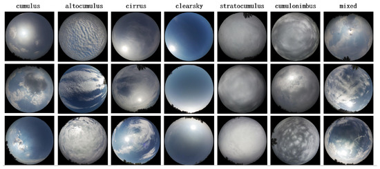
Figure 5.
Samples with each for one of the seven classes of cloud pictures.
The occluded testing samples are demonstrated in Figure 6.
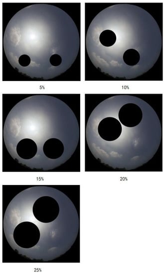
Figure 6.
The cloud samples with various percentage occlusion on MGCD.
4.2. Parameter Setting
Random partition ensures that the learning features will be uniformly distributed, while non-random allocation leads to uneven samples, which will seriously affect the convergence of network training phase and the generalization of network testing phase. Therefore, the data set is randomly divided into training set and testing set. The first one contains 2/3 of the cloud samples of each class, and the second one contains 1/3 of the cloud samples of each class.
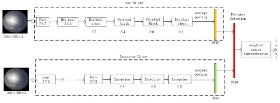
All experiments are carried out with the same experimental setup. We use transfer learning to train the convolutional neural network models of Inception-v3 network and ResNet-50 network. We change the size of the fully connected output layer to fit the cloud categories, and the input cloud samples are automatically cropped to input layer size.
A small batch random gradient descent method is used to adjust the parameters continuously, we set minimum batch size to 10, maximum epochs to 6, initial learn rate to 0.00001, validation frequency to 250.
4.3. Results
We will examine five methods for classifying ground-based Clouds, among which there are two existing ones:
- ICNN—using the Inception-v3 convolutional neural network (ICNN) for feature extraction and classification;
- RCNN—it is similar to ICNN, but the CNN used is the ResNet-50 convolutional neural network.
Three methods that we proposed:
- IWSRC—using the Inception-v3 convolutional neural network for feature extraction and the weighted sparse representation coding for classification;
- RWSRC—exactly the same as IWSRC but with the Inception-v3 CNN replaced by the ResNet-50;
- RIWSRC—this is the proposed two-channel CNN-based sparse representation coding method, depicted in Figure 4.
Train loss of convolutional neural network is displayed in Figure 7.
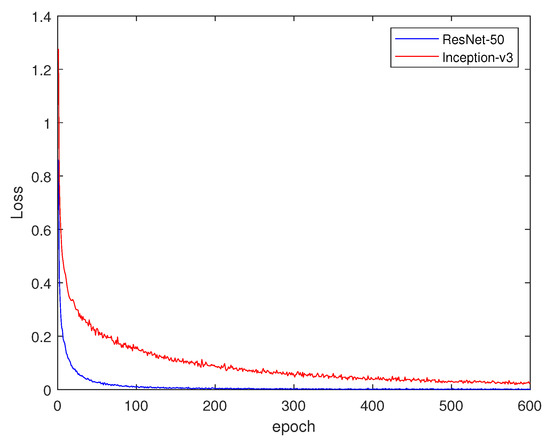
Figure 7.
Train loss of the two convolutional neural networks. An epoch means one complete pass of the training dataset through the algorithm.
Train accuracy of convolutional neural network is shown in Figure 8.
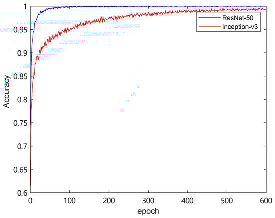
Figure 8.
Train accuracy of the two convolutional neural networks.
Table 4 shows the accuracy of all the methods used in this paper without occlusion.
Table 4.
The accuracy(%) of all the methods used in this paper without occlusion.
Table 5 shows the accuracy of each method when the occluded cloud samples are used.
Table 5.
The accuracy(%) of all the methods used in this paper with occlusion.
4.4. Discussion
In Figure 7, the overall trend is downward, and generally the loss of RCNN is lower than that of ICNN. In Figure 8, the recognition rate of RCNN is faster than that of ICNN.
As see Table 4, the RCNN is better than the ICNN since the ResNet-50 increases gradient propagation and hence is more effective in clouds classification. As to the proposed methods IWSRC, RWSRC and RIWSRC, they are all better than ICNN and RCNN because the noise interference can be suppressed with weighted representation learning during classification. However, RIWSRC achieves the best performance with the optimized feature selection process. The testing cloud images are with 5%, 10%, 15%, 20% and 25% occlusion, respectively.
In Table 5, experimental results with various occlusion show that the proposed IWSRC and RWSRC are better than ICNN and RCNN. The neural network is sensitive to perturbation with occlusion, and weighted sparse representation(WSR) will adjust the weights according to the size of the error. The larger error leads to smaller weights, which helps to reduce the perturbation on classification. In general, the proposed RIWSRC is more robust and effective than both IWSRC and RWSRC. The multiple features fusion can further improve the robustness of the algorithm The code is now publicly available on https://github.com/tangming666/NRC (accessed on 18 July 2021).
5. Conclusions
A novel robust classification scheme is proposed for ground-based clouds in this paper. The basic idea behind this is to use the CNNs for feature extraction and a weighted sparse representation coding for classification. Two classification algorithms are proposed directly along this line and the third one is based on the fusion of two CNNs. Experimental results show that the three proposed algorithms can enhance the robustness greatly. The proposed methods can be applied in most of deep learning neural networks.
As future research, we will consider adding some multimodal information to the selected neural network features to improve the robustness of the system. More applications of the proposed methods will be explored.
Author Contributions
All authors made significant contributions to the manuscript. A.Y. and M.T. conceived, designed and performed the experiments; G.L. wrote the paper; B.H. performed the experiments and analyzed the data; Z.X., B.Z. and T.C. revised the paper and provided the background knowledge of cloud classification. All authors have read and agreed to the published version of the manuscript.
Funding
This research received no external funding.
Institutional Review Board Statement
No applicable.
Informed Consent Statement
No applicable.
Data Availability Statement
The models and code used during the study are available in a repository (https://github.com/tangming666/NRC, accssed on 1 August 2021). The data is available from the corresponding author by request (shuangliu.tjnu@gmail.com).
Acknowledgments
This work was supported by Key Research & Development Project of Zhejiang Province 2021C04030 & the Public Project of Zhejiang Province LGG20F020007 and LGG21F030004. We would like to express my gratitude to Liu Shuang for providing the MGCD datasets. Our deepest gratitude goes to the reviewers for their careful work and thoughtful suggestions that have helped improve this paper substantially.
Conflicts of Interest
The authors declare no conflict of interest. The founding sponsors had no role in the design of the study; in the collection, analyses, or interpretation of data; in the writing of the manuscript, and in the decision to publish the results.
References
- Buch, K.A., Jr.; Sun, C.H.; Thorne, L.R. Cloud classification using whole-sky imager data. Ninth Symp. Meteorol. Obs. Instrum. 1996, 4, 353–358. [Google Scholar]
- Singh, M.; Glennen, M. Automated ground-based cloud recognition. Pattern Anal. Appl. 2005, 8, 258–271. [Google Scholar] [CrossRef]
- Heinle, A.; Macke, A.; Srivastav, A. Automatic cloud classification of whole sky images. Atmos. Meas. Tech. 2010, 3, 557–567. [Google Scholar] [CrossRef] [Green Version]
- Neto, S.L.M.; Wangenheim, R.V.; Pereira, R.B. The use of euclidean geometric distance on rgb color space for the classification of sky and cloud patterns. J. Atmos. Ocean. Technol. 2010, 27, 1504–1517. [Google Scholar] [CrossRef] [Green Version]
- Liu, S.; Wang, C.; Xiao, B.; Zhang, Z.; Shao, Y. Ground-based cloud classification using multiple random projections. In Proceedings of the 2012 International Conference on Computer Vision in Remote Sensing (CVRS), Xiamen, China, 16–18 December 2013. [Google Scholar] [CrossRef]
- Papin, C.; Bouthemy, P.; Rochard, G. Unsupervised segmentation of low clouds from infrared meteosat images based on a contextual spatio-temporal labeling approach. IEEE Trans. Geosci. Remote Sens. 2002, 40, 104–114. [Google Scholar] [CrossRef] [Green Version]
- Rathore, P.; Rao, A.S.; Rajasegarar, S.; Vanz, E.; Gubbi, J.; Palaniswami, M.S. Real-time urban microclimate analysis using internet of things. IEEE Internet Things J. 2017, 5, 500–511. [Google Scholar] [CrossRef]
- Holdaway, D.; Yang, Y. Study of the effect of temporal sampling frequency on DSCOVR observations using the GEOS-5 nature run results (part i): Earth’s radiation budget. Remote Sens. 2016, 8, 98. [Google Scholar] [CrossRef] [Green Version]
- Mahrooghy, M.; Younan, N.H.; Anantharaj, V.G. On the use of a cluster ensemble cloud classification technique in satellite precipitation estimation. IEEE J. Sel. Top. Appl. Earth Obs. Remote Sens. 2012, 1, 1356–1363. [Google Scholar] [CrossRef]
- Tan, K.; Zhang, Y.; Tong, X. Cloud extraction from chinese high resolution satellite imagery by probabilistic latent semantic analysis and object-based machine learning. Remote Sens. 2016, 8, 963. [Google Scholar] [CrossRef] [Green Version]
- Liu, L.; Sun, X.; Chen, F.; Zhao, S.; Gao, T. Cloud Classification Based on Structure Features of Infrared Images. J. Atmos. Ocean. Technol. 2011, 410–417. [Google Scholar] [CrossRef]
- Yang, J.; Lu, W.; Ma, Y.; Wen, Y. An Automatic Ground-based Cloud Detection Method Based on Adaptive Threshold. J. Appl. Meteorol. Sci. 2009, 20, 713–721. [Google Scholar]
- Liu, S.; Wang, C.; Xiao, B.; Zhang, Z.; Cao, X. Tensor Ensemble of Ground-Based Cloud Sequences: Its Modeling, Classification, and Synthesis. IEEE Geosci. Remote. Sens. Lett. 2013, 10, 1190–1194. [Google Scholar] [CrossRef]
- Lecun, Y.; Bottou, L. Gradient-based learning applied to document recognition. Proc. IEEE 1998, 86, 2278–2324. [Google Scholar] [CrossRef] [Green Version]
- Krizhevsky, A.; Sutskever, I.; Hinton, G. Imagenet classification with deep convolutional neural networks. Adv. Neural Inf. Process. Syst. 2012, 25, 1097–1105. [Google Scholar] [CrossRef]
- Szegedy, C.; Vanhoucke, V.; Ioffe, S. Rethinking the inception architecture for computer vision. In Proceedings of the 2016 IEEE Conference on Computer Vision and Pattern Recognition, Las Vegas, NV, USA, 27–30 June 2016. [Google Scholar]
- He, K.; Zhang, X.; Ren, S.; Sun, J. Deep residual learning for image recognition. In Proceedings of the 2016 IEEE Conference on Computer Vision Foundation, Las Vegas, NV, USA, 27–30 June 2016; pp. 770–778. [Google Scholar]
- Liu, S.; Li, M. Deep multimodal fusion for ground-based cloud classification in weather station networks. Eurasip J. Wirel. Commun. Netw. 2018, 2018, 48. [Google Scholar] [CrossRef] [Green Version]
- Liu, S.; Li, M.; Zhang, Z.; Xiao, B.; Cao, X. Multimodal ground-based cloud classification using joint fusion convolutional neural network. Remote Sens. 2018, 10, 822. [Google Scholar] [CrossRef] [Green Version]
- Donoho, D.L. Compressed sensing. IEEE Trans. Inf. Theory 2006, 52, 1289–1306. [Google Scholar] [CrossRef]
- Kutyniok, G. Theory and applications of compressed sensing. GAMM-Mitteilungen 2013, 36, 79–101. [Google Scholar] [CrossRef] [Green Version]
- Elad, M.; Aharon, M. Image denoising via sparse and redundant representations over learned dictionaries. IEEE Tip 2006, 15, 3736–3745. [Google Scholar] [CrossRef] [PubMed]
- Mairal, J.; Elad, M.; Sapiro, G. Sparse representation for color image restoration. IEEE Trans. Image Process. 2007, 17, 53–69. [Google Scholar] [CrossRef] [PubMed] [Green Version]
- Wright, J.; Ma, Y. Dense error correction via l1-minimization. In Proceedings of the IEEE International Conference on Acoustics, Speech and Signal Processing, Taipei, Taiwan, 19–24 April 2009. [Google Scholar]
- Yang, M.; Zhang, L. Gabor feature based sparse representation for face recognition with gabor occlusion dictionary. In Proceedings of the 11th European conference on Computer Vision, Crete, Greece, 5–11 September 2010; pp. 448–461. [Google Scholar]
- Yang, M.; Zhang, L.; Yang, J. Robust sparse coding for face recognition. In Proceedings of the CVPR 2011, Colorado Springs, CO, USA, 20–25 June 2011; Volume 42, pp. 625–632. [Google Scholar]
- Gan, J.; Lu, W.; Li, Q.; Zhang, Z.; Yang, J.; Ma, Y.; Yao, W. Cloud type classification of total-sky images using duplex norm-bounded sparse coding. IEEE J. Sel. Top. Appl. Earth Obs. Remote Sens. 2017, 10, 3360–3372. [Google Scholar] [CrossRef]
- Szegedy, C.; Liu, W.; Jia, Y.; Sermanet, P.; Reed, S.; Anguelov, D.; Erhan, D.; Vanhoucke, V.; Rabinovich, A. Going deeper with convolutions. In Proceedings of the 2015 IEEE Conference on Computer Vision and Pattern Recognition (CVPR), Boston, MA, USA, 7–12 June 2015; pp. 1–9. [Google Scholar]
Publisher’s Note: MDPI stays neutral with regard to jurisdictional claims in published maps and institutional affiliations. |
© 2021 by the authors. Licensee MDPI, Basel, Switzerland. This article is an open access article distributed under the terms and conditions of the Creative Commons Attribution (CC BY) license (https://creativecommons.org/licenses/by/4.0/).